Classification of knee osteoarthritis based on quantum-to-classical transfer learning

Quantum machine learning takes advantage of features such as quantum computing superposition and entanglement to enable better performance of machine learning models. In this paper, we first propose an improved hybrid quantum convolutional neural network (HQCNN) model. The HQCNN model was used to pre-train brain tumor dataset (MRI) images. Next, the quantum classical transfer learning (QCTL) approach is used to fine-tune and extract features based on pre-trained weights. A hybrid quantum convolutional network structure was used to test the osteoarthritis of the knee dataset (OAI) and to quantitatively evaluate standard metrics to verify the robustness of the classifier. The final experimental results show that the QCTL method can effectively classify knee osteoarthritis with a classification accuracy of 98.36%. The quantum-to-classical transfer learning method improves classification accuracy by 1.08%. How to use different coding techniques in HQCNN models applied to medical image analysis is also a future research direction.

1 Introduction

Osteoarthritis (OA) is one of the most common forms of arthritis, and it is an important factor limiting mobility and limb function in the elderly Hunter et al. [1]. The etiology of osteoarthritis is unknown, and its advanced features are characterized by cartilage wear, bone deformity, and synovitis Mobasheri and Batt [2], Mathiessen and Conaghan [3]. Imaging is the most important tool for detecting osteoarthritis and can identify early signs of osteoarthritis and slow disease progression through behavioral interventions (e.g., exercise and weight loss programs) Baker and McAlindon [4]. MRI (magnetic resonance imaging) can reflect the three-dimensional structure of the knee joint. However, the small number and high cost of MRI testing equipment make it unsuitable for the routine diagnosis of osteoarthritis. Kellgren–Lawrence (KL) system is one of the most commonly used clinical scales to assess the severity of osteoarthritis by X-ray/ plain radiography Kellgren and Lawrence [5]. However, the consistency of visual diagnosis by radiologists is low, thus introducing significant inconsistencies in decision-making Tiulpin et al. [6]. Doctors usually examine scanned X-ray images of the knee joint and then grade the KL of both knees in a short period of time. The accuracy of the diagnosis significantly relies on the experience and care of the physician. In addition, as shown in Figure 1, the criteria for KL classification are very vague. For example, KL grade 1 is determined by possible bone graft lip and joint space narrowing (JSN). Even the same physician may give different KL grades when examining the same knee at different points in time. In a study conducted by Culvenor et al., the reliability of those scoring within KL ranged from 0.67 to 0.73 Simonyan and Zisserman [7].

FIGURE 1

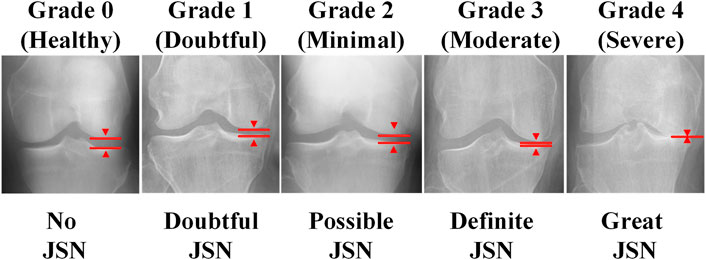
FIGURE 1. The KL system classifies the severity of osteoarthritis of the knee into five levels, from 0 to 4.

In recent years, deep learning has become a major research direction for assessment of osteoarthritis severity. Due to the high prevalence of osteoarthritis, there is an urgent need for methods to accurately detect its presence and quantify its severity. Fully automated osteoarthritis severity grading can provide objective and reproducible predictions. Over the past decade, several methods have been developed for the detection of the knee joint and the classification of KL grades. Antony designed a new convolutional neural network (CNN) model for the KL grading task and optimized the weighted combination of cross-entropy loss and mean square error loss to obtain a recognition rate of 63.6% Antony et al. [8]. Tiulpin et al. [6] and Antony et al. [9] divided the osteoarthritis assessment task into two phases, detection and classification, in which faster region-based convolutional neural networks (R-CNNs) Yang et al. [10] were used for detection, and a deep convolutional network was used for classification. Albert Swiecicki et al. [11]developed an automated algorithm based on deep learning to jointly use posterior–anterior (PA) and lateral (LAT) views of knee X-rays to assess the severity of knee osteoarthritis according to the KL grading system. Zhang et al. [12]proposed a CNN KL grade classification model for knee osteoarthritis under the attention mechanism, applying ResNet to first extract knee features from X-rays and then combine them with the features extracted by the convolutional attention module to automatically perform KL grade prediction.

Quantum machine learning algorithms are particularly suitable for diagnostic applications. Many potentially related variables lead to high-dimensional feature spaces, and interactions between variables lead to complex interdependencies, correlations, and patterns. Quantum machine learning algorithms are able to penetrate such data structures in ways that go beyond purely classical methods. Therefore, a wide range of quantum applications are being explored in this field, including processing steps such as enhanced image edge detection, segmentation, and classification Bharti et al. [13]. Landman et al. [14] studied orthogonal quantum-assisted neural network (QNN) in retinal color fundus and chest X-ray image classification and used quantum circuits to accelerate the training of classical neural networks. Kiani et al. [15] developed a quantum Fourier transform (qFT)-based enhanced image reconstruction algorithm based on computed tomography (CT) and positron emission tomography (PET) data. For breast cancer image classification, Azevedo et al. [16] applied quantum enhanced SVM classifiers (QSVCs) and transfer learning-based QNNs. Moradi et al. [17] used a quantum kernel Gaussian process approach. Ahalya et al. [18] classified rheumatoid arthritis heat maps using quantum kernel alignment-trained QSVCs. Shahwar et al. [19] detailed the classification of MRI images of Alzheimer’s disease using QNNs. Houssein et al. [20] classified chest X-ray images with QNNs. Sengupta and Srivastava [21] classified COVID-19 CT lung images with QNNs Bergholm et al. [22].

The main research innovations in this paper are as follows:

1) Design of a hybrid quantum convolutional neural network structure (HQCNN) for multi-classification of MRI images. The basic idea is to encode data into quantum states so that information can be extracted faster and then use the information to distinguish classes of data. The quantum convolutional network consists of a Quantum Convolutional Layer (QCL) and a classical convolutional layer. The QCL consists of an encoder, a random circuit, and a decoder. The classical convolutional layer consists of a classical convolutional layer, a global pooling layer, and a dense layer.

2) The quantum-to-classical (QC) transfer learning scheme is selected based on the labeling of MRI images and OAI images and the relationship between MRI image classification and OAI grading tasks. The QC transfer learning is divided into two phases: pre-training and fine-tuning. The pre-training phase uses the already trained quantum neural network model to learn quantum state evolution and quantum gate operations. 2) The fine-tuning phase applies the pre-trained model to a new task and further tunes and trains the model in the new task.

3) Most current hybrid quantum convolutional network structures use variational quantum circuits for the final classification. We propose the HQCNN algorithm to downscale classical image data before encoding them into quantum lines. The pre-processed data are encoded into quantum data by a data encoding line.

2 Hybrid quantum convolutional neural network

In this section, we propose a HQCNN, as shown in Figure 2. The use of full quantum algorithms is currently not feasible due to technical bottlenecks caused by high coherence requirements, quantum noise, and limited number of quantum bits. Hybrid computing Henderson et al. [23] uses a best-of-both-worlds approach to solve a particular problem. In fact, the idea behind including quantum circuits in neural networks is to leverage the performance of the network for faster scaling and minimal training.

FIGURE 2

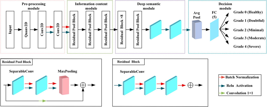
FIGURE 2. Hybrid quantum convolutional neural network.

To better describe our HQCNN structure, we first give a brief overview of some basic features of CNNs. The classical transfer learning consists of interleaved convolutional and pooling layers and ends with a fully connected layer. The main purpose of the convolutional layer is to extract features from the input data using a feature mapping (or filter), which is the most computationally intensive step in a CNN. A pooling layer is usually added after the convolutional layer to reduce the dimensionality of the data and prevent overfitting. The basic idea of quantum CNN structure is to encode data into quantum states so that information can be extracted faster and then use the information to distinguish classes of data. The hybrid quantum CNN consists of a QCL and a classical convolutional layer. The QCL has three parts: an encoder, a random circuit, and a decoder. After obtaining the output from the QCL, the information is passed to the classical convolutional layer of the architecture. The classical convolutional layer consists of three different layers, namely, the classical convolutional layer, the global pooling layer, and the dense layer.

2.1 Quantum convolution layer

The QCL performs sequential parsing of images and extracts local information, features, and patterns from the images, which makes an important contribution to image classification. As mentioned previously, the current work follows the hybrid quantum classical approach proposed by Henderson et al Abohashima et al. [24]. Henderson Abohashima et al. [24] provided a quantum analog of the classical convolutional layer and named it the “quantum convolution” layer. Similar to the classical convolutional layer, the proposed layer extracts high-level spatial features from the input image. The layer consists of a quantum circuit that encodes pixel data on n × n quantum bits (where n denotes the kernel size), applies a random quantum circuit on these bits, and then measures them to produce a feature matrix. Henderson et al. used thresholds to encode pixel values greater than the pixel value encoded as, and pixel values less than or equal to the threshold are encoded as |0>. The internal structure of the quantum convolution layer is shown in Figure 3.

FIGURE 3

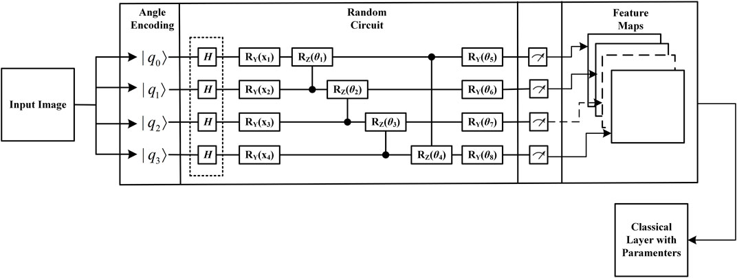
FIGURE 3. Quantum convolution layer.

2.1.1 Encoder

During the encoding process, the pixel data corresponding to the filter size are stored in the form of quantum bits. Encoding images into quantum circuits is a challenging task in the field of quantum machine learning Schuld [25]. There are five quantum coding approaches to encode data points into a quantum circuit, namely, ground state coding Havlíček et al. [26], angular coding Havlíček et al. [26], amplitude coding Havlíček et al. [26], IQP coding Huang et al. [27], and Hamiltonian quantum evolution coding Mari et al. [28]. A simple encoding idea is to convert a data point into an angle in a quantum state (in fact, quantum bit elements are state vectors representing data points as angles attributed to different directions of the state vector). Each quantum bit depends on its classical data point to represent its configuration. Angular encoding Havlíček et al. [26] is the encoding of classical information using the rotation angles of the revolving doors R_x, R_y, and R_z. The rotation matrix is defined as follows:

$R_x\left(\theta \right)=\left[\begin{array}{cc}\hfill \cos \frac{\theta }{2}\hfill & \hfill -i\sin \frac{\theta }{2}\hfill \\ \hfill -i\sin \frac{\theta }{2}\hfill & \hfill \cos \frac{\theta }{2}\hfill \end{array}\right],(1)$

$R_y\left(\theta \right)=\left[\begin{array}{cc}\hfill \cos \frac{\theta }{2}\hfill & \hfill -\sin \frac{\theta }{2}\hfill \\ \hfill \sin \frac{\theta }{2}\hfill & \hfill \cos \frac{\theta }{2}\hfill \end{array}\right],(2)$

$R_z\left(\theta \right)=\left[\begin{array}{cc}\hfill e^{-i\frac{\theta }{2}}\hfill & \hfill 0\hfill \\ \hfill 0\hfill & \hfill e^{i\frac{\theta }{2}}\hfill \end{array}\right].(3)$

These are the effective operators on the Bubbleley spin matrices. Essentially, the gate R_x(θ) rotates the state vector in space by one angle with respect to the x-axis. Similarly, gate R_y and gate R_z are related to the y-axis and z-axis, respectively. The angle θ corresponds directly to the intensity value of a pixel. After mapping all data points to quantum bits, the random q-circuit can be designed using the operations of quantum bits and quantum gates. Angular encoding, on the other hand, encodes N classical data onto N quantum bits.

$|\mathbf{x}\rangle =\underset{i=1}{\overset{N}{\otimes }}\cos \left(x_i\right)|0\rangle +\sin \left(x_i\right)|1\rangle ,(4)$

where |x⟩ is the classical data vector to be encoded. However, a qubit can be loaded not only with angular information but also with phase information. Therefore, it is perfectly possible to encode a classical data of length N onto N quantum bits.

$|\mathbf{x}\rangle =\underset{i=1}{\overset{\left[N/2\right]}{\otimes }}\cos \left(\pi x_{2i-1}\right)|0\rangle +e^{2\pi i{x}_{2i}}\sin \left(\pi x_{2i-1}\right)|1\rangle ,(5)$

where the two data are encoded into the rotation angle $\cos \left(\pi x_{2i-1}\right)|0\rangle$ and phase information $e^{2\pi i{x}_{2}i}\sin \left(\pi x_{2i-1}\right)|1\rangle$ of the quantum special, respectively.

2.1.2 Random circuit

A series of uniform quantum transformations (implemented through the gates defined earlier) and measurements of quantum bit elements are essential to design a quantum circuit. The quantum convolution layer contains quantum kernels. It essentially segments the input image into smaller patches containing local information by using a q-circuit to detect and extract meaningful spatial information and features from the image. The idea of having a simple depth and using smaller quantum bit elements is to integrate a random q-circuit in the QCL. The random circuit is composed of randomly selected single and double quantum bit gates. The rotation applied to these doors is also chosen randomly using Numpy’s random method. We design parametric quantum circuits, which are composed of interleaved single and double quantum bit layers. The single quantum bit layer consists of R_y gates, each containing a tunable parameter. Using the Adama gate, the quantum bits are initialized with a balanced superposition of |0⟩ and |1⟩, and then the quantum bits are rotated according to the input parameters. The main purpose of the embedding operation is to initialize the quantum bits by properly balancing the |0⟩ and |1⟩ quantum bit values using input-based Adama gates and rotation gates. The quantum coding framework is responsible for establishing the association between the classical information input x and its associated quantum state |X⟩. In general, quantum coding implements quantum embedding, converting classical input vectors into quantum state vectors. The resulting quantum state is given by the following equation.

$\begin{array}{cc}\hfill & |Z\rangle =|z_1\rangle \otimes |z_2\rangle \otimes |z_3\rangle \otimes |z_4\rangle \hfill \\ \hfill & \left({\otimes }_{i=1}^4{R}_Y\left(2z_i\right)\right)|{0\rangle }^{\otimes 4}.\hfill \end{array}(6)$

The quantum coding circuit develops new quantum states, as shown in Eq. 7.

$\left({\otimes }_{i=1}^4{R}_Y\left(\pi z_i\right)\right)|{0\rangle }^{\otimes 4}.(7)$

The quantum variational layer consists of a series of rotational layers consisting of rotational gates followed by an entanglement layer consisting of CNOT gates to satisfy the training process. During the operation, the CNOT gate enforces quantum manipulation of the entanglement between any neighboring quantum lines, resulting in the entanglement of quantum bits in each quantum line. Meanwhile, the rotation angle of the revolving door is adjustable. During training, the data are transmitted through a variational layer consisting of alternating rotating gates and entangled gates (control but not control gates). The best performance model for the proposed work includes a quantum depth of 4 in this variational quantum circuit, as shown in Eq. 8.

$X=L_{4o\dots \dots \dots }{L}_{2o}{L}_1.(8)$

2.1.3 Decoder

This component of the QCL is responsible for all measurements that occur in this layer. Decoding indicates the measurement of quantum data, and the data are converted to classical form. The measured data provide relevant information about the images, which can then be fed into the neural network in order to classify the types of images. The bubble spin matrices are used in this component. They are the most intuitive and simplest way to decode quantum information and generate the corresponding classical information. The data decoder component measures the data along the z-axis by using the Pauli-Z matrix defined previously. Depending on the selected measurement operator, we commonly classify the measurements into computational base measurements, projective measurements, Pauli measurements, etc. Pauli measurements are projective measurements in which the sizable measurement M is selected as the bubble operator. Taking the Pauli-Z measure as an example, we consider the Z-operator:

$Z=\left(\begin{array}{cc}\hfill 1\hfill & \hfill 0\hfill \\ \hfill 0\hfill & \hfill -1\hfill \end{array}\right).(9)$

It can be seen that Z satisfies Z = Z^†, i.e., Z is Hermitian. Z has two eigenvalues +1, −1 and the corresponding eigenvectors are |0⟩ and |1⟩. Thus, the spectral decomposition of Z takes the form

$\begin{array}{cc}\hfill & \hfill \\ \hfill & Z=\left(\begin{array}{cc}\hfill 1\hfill & \hfill 0\hfill \\ \hfill 0\hfill & \hfill -1\hfill \end{array}\right)=1\times |0\rangle \langle 0|+\left(-1\right)\times |1\rangle \langle 1|\hfill \end{array}.(10)$

We use Z for projection measurement, if the measurement is +1. We can conclude that the state of this quantum bit is projected into the +1 characteristic subspace V₊₁ of the Z operator, indicating that the measured state is projected into |0⟩. Similarly, if the measurement result is −1, it can be concluded that the quantum bit is projected into the −1 eigenspace V₋₁, indicating that the measured state is projected into |1⟩.

After quantum transformation, the data are in an arbitrary quantum state, and the output quantum state needs to be measured to obtain classical information for subsequent processing. The quantum decoding (measurement) operation is a nonlinear transformation that implements a function similar to the classical activation function. The classical data obtained from the measurements will be used in the subsequent classical part of the convolutional neural network where each quantum bit is measured and then a vector is generated and fed into the corresponding quantum feature map. A quantum bit element generates a quantum feature map, which corresponds to a channel. When the sliding window of the input image is completed, the quantum feature map of that image is formally generated and serialized and saved to a disk for classifier training.

3 Quantum-to-classical transfer learning

3.1 Classical-to-quantum transfer learning solutions

Traditionally, deep neural networks require large labeled datasets and powerful computational resources to solve challenging computer vision problems, such as feature extraction and classification. Transfer can be used to learn a new task by transferring knowledge from a related learning task. From a pre-trained model, we perform two tasks: 1) fine-tuning 2) and feature extraction in the fine-tuning. Essentially, the model is retrained to update most or all of the parameters based on the pre-trained weights. In feature extraction, the weights of the last layer (classifier) are trained using the coding features of the pre-trained model. Deriving predictions and reconstructing a new dataset with the same number of output classes implies that the pre-trained HQCNN model acts as a fixed-function extractor. In this case, a pre-trained quantum network is a kind of feature extractor, resulting in an output vector of values associated with the input. The extracted features are then further processed using classical networks to solve the specific problem of interest. A generic transfer learning scheme is shown in Figure 4.

Step 1: Take a network A that has been pre-trained on the dataset D_A and the given task T_A.

Step 2: By deleting some final layers, the resulting truncated network A’ can be used as a feature extractor.

Step 3: A new trainable network B is connected at the end of the pre-trained network A’.

Step 4: Keep the weights of A’ constant and train the final block B with a new dataset D_B and a new task T_A of interest.

FIGURE 4

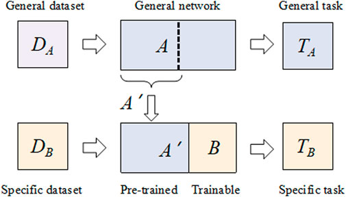
FIGURE 4. Generic transfer learning scheme Deng et al. [35].

3.2 Quantum-to-classical transfer learning programs

Quantum-to-classical transfer learning involves using pre-trained quantum circuits as feature extractors and post-processing their output variables using classical neural networks. In this case, only the final classical part will be trained to the specific problem of interest. In our problem, this can be translated as shown in Table 1. The quantum classical transfer learning (QCTL) scheme is shown in Figure 5. An important criterion for using pre-trained HQCNN models is the use of appropriate image pre-processing. The image corresponds to a data point that needs to be encoded, and it first needs to be reshaped to reduce the number of quantum bits in the circuit. In addition, the pixels are rescaled to (H, W, C) = (128, 128, 1) before normalizing them to 1. Standardization is the process of converting pixel values 0–255 to real numbers in the range 0.0–1.0. This has the advantage of reducing the amount of computation while improving computational accuracy.

TABLE 1

TABLE 1. Quantum-to-classical transfer learning scheme.

FIGURE 5

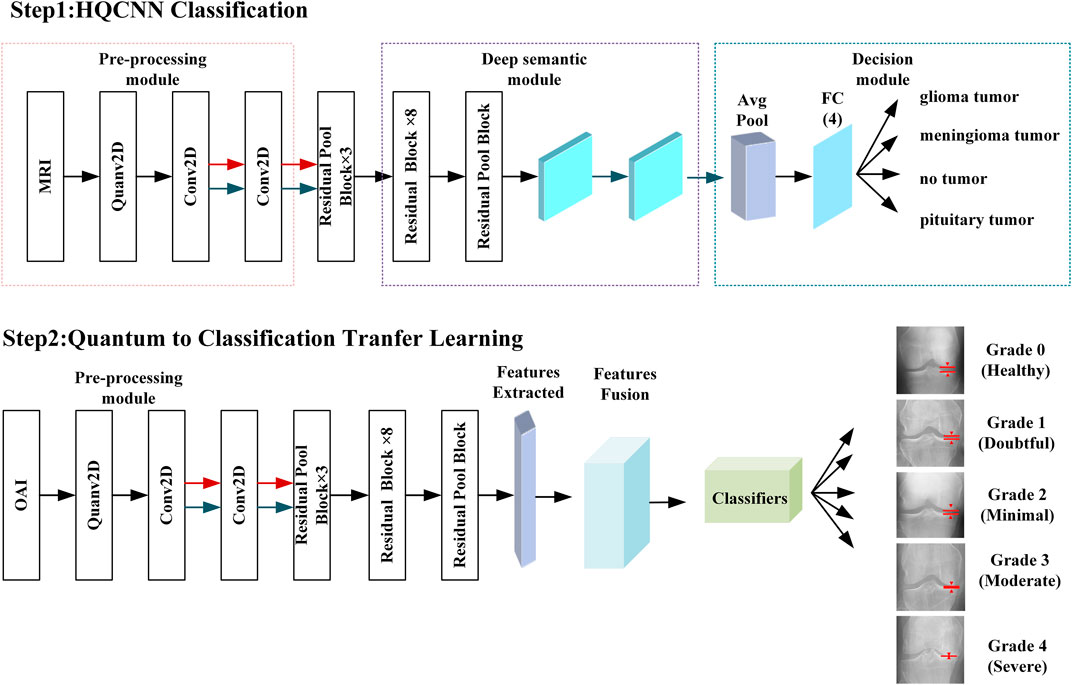
FIGURE 5. Quantum-to-classical transfer learning scheme.

Step 1: Qubit Lattice Latorre [29], Le et al. [30], Real Ket Le et al. [30], and FRQI Chen [31] are the three main quantum image formats. The quantum image format, Real Ket, was proposed by Latorre Le et al. [30]. In this format, an image is divided into four blocks, each numbered from left to right, starting from the top row. These blocks are again subdivided into four blocks and numbered in the same way until the smallest block with only four pixels is obtained. The grayscale values of these four pixels are mapped to the probability amplitude of each component of a quantum state with two quantum bit elements. Eq. 11 describes the quantum state, where i₁ = 1 is the index of the top-left pixel, i₁ = 2 is the index of the top-right pixel, i₁ = 3 is the bottom-left pixel, and i₁ = 4 is the bottom-right pixel.

C_i stores the mapped value of each pixel and satisfies ${\sum }_{i_1=\mathrm{1,2},\dots 4}|C_{i_1}{|}^2=1$

$\begin{array}{c}|{\psi }_{2^{1}X{2}^1}\rangle =\sum _{i_1=\mathrm{1,2},..4}{C}_{i_1}|{\text{i}}_1\rangle \\ \mathbf{\text{such that}}\sum _{i_1=\mathrm{1,2}..4}{\left|C_{i_1}\right|}^2=1.\end{array}(11)$

We now consider a larger block consisting of four internal sub-blocks. In order to determine which sub-block we are dealing with, a new label, called i₂, is needed with the same conventions as those defined for the internal blocks. The new image shows 2² × 2² pixels and is represented by the real vector in R⁴ ⊗ R⁴:

$|{\psi }_{2^2\times 2^2}\rangle =\sum _{i_1,i_2=1,\dots 4}{c}_{i_2,i_1}|i_2,i_1\rangle ,(12)$

where $c_{i_2,i_1}$ stores all the pixel values.

This block structure can be extended in any number of steps to a size of 2² × 2²pixels. By gradual extension, an image of 2² × 2² pixels can be mapped to a quantum state, as shown in the following equation:

$\begin{array}{cc}\hfill & |image|=|{\psi }_{2^{n+2^n}}\rangle =\sum _{i_n\dots i_1=1,\dots ,4}{C}_{i_n\dots i_1}|i_n,\dots ,i_1\rangle \hfill \\ \hfill & \text{such\hspace{0.17em}that}\sum _{i_n\dots .i_1=1,\dots ,4}{\left|C_{i_n\dots i_1}\right|}^2=1.\hfill \end{array}(13)$

Step 2: Feature extraction is the extraction of valuable features from an image. Instead of extracting manual features, the QCNN now automatically extracts important features from images. In this work, we use the pre-trained HQCNN model proposed in this paper as a feature extractor. The classical layer of the HQCNN model uses the Xception network, which uses a residual learning strategy that is effective enough. The residual blocks of the Xception architecture are described as follows.

$\mathrm{g}=\mathrm{F}\left(\mathrm{h},\mathrm{W}+\mathrm{h}\right),(14)$

where h is the input layer, g is the output layer, and the F function is represented by the residual mapping.

Step 3: The feature dimensions extracted from the HQCNN model are executed on the classical layer, i.e., there is a linear transformation from 512 features to 64 features. Classical output features from the classical convolutional layer are passed to the final fully connected layer to create two-dimensional target output class predictions. The output is the target class of the five classification problems predicted by the model.

$\tilde{K}=L_{{512\to 64}^{◦}}{K}_{{◦}_{L_{64}\to 5}}.(15)$

4 Datasets and pre-processing

4.1 Splitting the dataset

The two datasets used in this paper are from Kaggle, and the brain tumor dataset includes MRI images of brain tumors from 233 patients. There were 926 glioma tumor sections, 937 meningioma tumor sections, 500 tumor-free sections, and 901 pituitary tumor sections, for a total of 3,264 images. The distribution of the MRI data set is shown in Table 2. The images used to evaluate knee X-rays were obtained from the Osteoarthritis Initiative Quinonero-Candela et al. [32], a multicenter, longitudinal, prospective observational study of osteoarthritis of the knee designed to identify biomarkers of OAI onset and progression. A total of 4,796 participants aged 45–79 years participated in this test. The publicly available dataset from Chen et al Quinonero-Candela et al. [32] was used in our study. The knee dataset contains 9,516 X-ray images, of which 3,857 are Grade 0 images, 1,770 are Grade 1, 2,578 are Grade 2, 1,286 are Grade 3, and 295 are Grade 4. The distribution of the OAI dataset is shown in Table 3.

TABLE 2

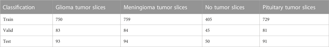
TABLE 2. MRI data and distribution.

TABLE 3

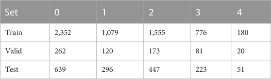
TABLE 3. OAI data and distribution.

4.2 Adversarial validation

Adversarial validation is a simple but effective method that essentially constructs a classification model to predict the probability of a sample being in the training or test set. If the classification of this model is good (generally the AUC is above 0.7), then it indicates that there is a large difference between the training and test sets. Figure 6 shows the MRI dataset before division. If the AUC score is close to 0.5, it means that the training and test sets have the same distribution. Figure 7 shows the MRI dataset after division, and Figure 8 shows the OAI dataset before division.

FIGURE 6

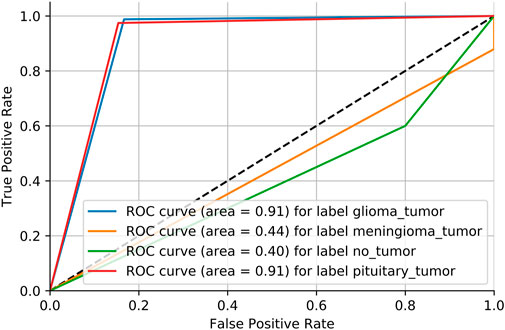
FIGURE 6. Training and test set ROC scores for each class of the MRI dataset before delineation.

FIGURE 7

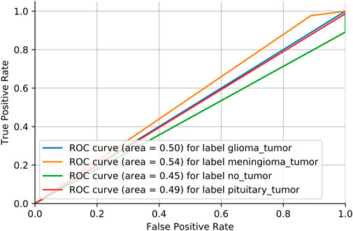
FIGURE 7. Training and test set ROC scores for each class of the delineated MRI dataset.

FIGURE 8

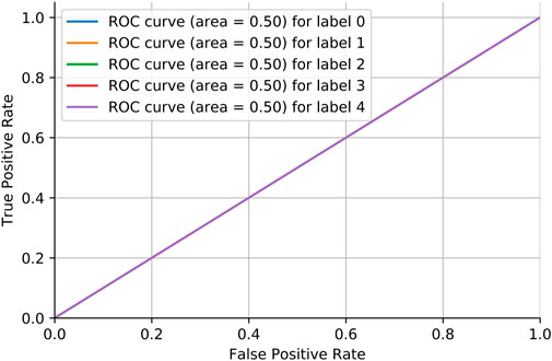
FIGURE 8. Training and test set ROC scores for each class of the pre-division OAI dataset.

We need to consider the variability of data distribution. Inconsistency between the training data distribution and the actual data distribution to be predicted is likely to lead to poor model performance, which is often referred to as a dataset shift Glorot and Bengio [33]. As shown in Figure 6, we consider repartitioning the training set and test set due to severe dataset shift in the MRI dataset. As shown in Figure 7, there is no dataset shift in the OAI dataset, and there is no need to repartition the training set and test set. The pairwise validation has the following steps:

Step 1: The index of each category of tumor is separated from the training set and the test set.

Step 2: A new label is prepared and tumor = 1 is set in the training set and tumor = 0 in the test set. Then, the tumors from the training set and the test set are spliced.

Step 3: The spliced dataset is shuffled, and then the tumor of each category is repartitioned according to train:test = 9:1.

Step 4: A random forest classifier is prepared with parameters set to bootstrap = True, oob_score = True, criterion = entropy for training.

Step 5: The trained classifiers are predicted against the test set, and their ROC scores are calculated.

4.3 k-fold cross-validation

The statistics in Table 3 show that Grade 0 and Grade 1 and Grade 2 images occupy the majority of the data set, while the number of Grade 3 and Grade 4 images is quite small. The highest number of Grade 0 images accounts for 39.4%, while the lowest number of Grade 4 images accounts for only 0.03%. Therefore, the data handled in this study are a typical unbalanced dataset. To ensure the consistency of the label distribution between the training and validation sets, we use the Stratified KFold method for the partitioning of the dataset. Stratified KFold is a stratified sampling cross-cut to ensure that the proportion of samples of each category in the training set and test set is the same as in the original dataset. The dataset is divided as follows: 1) 1/10 holdout set for ensemble and (2) building 5-fold cross-validation sets using rest of 9/10. Table 4 shows the 10-fold cross-validation of the OAI dataset.

TABLE 4

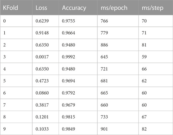
TABLE 4. Ten-fold cross-validation of the OAI dataset.

4.4 Evaluation indicators

We know that selecting a classifier with better performance requires the use of excellent evaluation metrics. To understand the generalization ability of the model, it must be evaluated using objective metrics, which is the importance of performance evaluation. In machine learning, a classification task involving more than two classes is called multiclass classification. We must be very careful when choosing evaluation metrics for multiclass, single-label classifiers. First, it is different from the binary class metrics. Second, it is important to consider whether the dataset is single-label or multi-label. In multiclass, there is only one label, while in multitag, there are multiple labels. Since OAI is multiclass, we chose a measure based on the concept of multiclass, individual labels.

4.4.1 Accuracy

Accuracy, one of the most popular metrics in multiclass classification, reflects the correct prediction of the sample score and can be calculated directly from the confusion matrix. Its calculation formula is as follows:

$Accuracy=\frac{TP+TN}{TP+TN+FP+FN}.(16)$

The model predicted that the true positive as positive, but it was actually positive. The model predicts false positives as positive, but it is actually negative. The calculation is also applicable to multiple classes and is very simple. To calculate accuracy, we simply add these elements to the diagonal of the confusion matrix and divide by the total number of labels.

4.4.2 Macro precision

Precision indicates how much we can trust the model when it predicts a positive outcome for an individual. The macroscopic precision of the multiclass algorithm is calculated in two steps. First, Eq. 17 is used to calculate the precision for each class, where k denotes the class.

$Precisio{n}_k=\frac{T{P}_k}{T{P}_k+F{P}_k}.(17)$

Next, the arithmetic mean of each class is calculated using Eq. 18, where K denotes the number of classes.

$MacroPrecision=\frac{\sum _{k=1}^{K}precisio{n}_k}{K}.(18)$

4.4.3 Macro recall

Macro recall for multiple classes, such as macro precision, requires a two-step calculation. First, Eq. 19 is used to calculate the recall for each class, where k denotes the class.

$Recall=\frac{T{P}_k}{T{P}_k+F{N}_k}.(19)$

Next, the arithmetic mean of each class is calculated using Eq. 20, where K denotes the number of classes.

$MacroRecall=\frac{\sum _{k=1}^{K}Recal{l}_k}{K}.(20)$

4.4.4 Macro F1 score

The macro-F1 score is a reconciled average of the macro-accuracy and macro-check-completion rates, taking into account both the accuracy and the check-completion rate of the classification model. Therefore, before calculating the macro f1 score, we must first calculate the macro precision and macro recall. The macro F1 score is calculated as follows:

$\text{\hspace{0.17em}Macro\hspace{0.17em}F}1\text{\hspace{0.17em}Score\hspace{0.17em}}=2\times \frac{\text{\hspace{0.17em}Macro\hspace{0.17em}Precision\hspace{0.17em}}\times \text{\hspace{0.17em}Macro\hspace{0.17em}Recall\hspace{0.17em}}}{\frac{1}{\text{\hspace{0.17em}Macro\hspace{0.17em}Precision\hspace{0.17em}}}+\frac{1}{\text{\hspace{0.17em}Macro\hspace{0.17em}Recall\hspace{0.17em}}}}.(21)$

To facilitate the observation of each class, we precisely compute the precision, recall, f1, and support of the class in both datasets, where support is the number of classes belonging to that class in the dataset without division. The classification report of the MRI dataset is shown in Figure 9, and the classification report of the OAI dataset is shown in Figure 10.

FIGURE 9

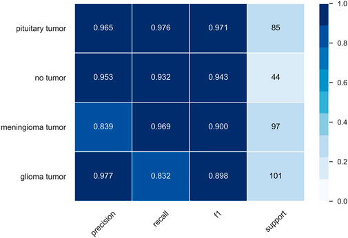
FIGURE 9. MRI classification report.

FIGURE 10

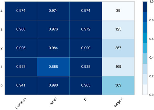
FIGURE 10. OAI classification report.

5 Comparison experiment

5.1 Experiment1 MRI classification

For the first phase of the experiment, we need to explain the weight initializer, loss function, and optimizer. The GlorotUniform initializer, also called Xavier uniform initializer, proposed by Glorot and Bengio [33], is used to initialize the convolutional kernel weights so that the variances of each layer are as equal as possible to achieve a better flow of information in the network. We know that for regression models, the commonly used loss function is the mean square error function, while for classification models that predict probabilities, the most commonly used loss function is cross-entropy. Therefore, we uniformly use categorical cross-entropy as the loss function. Categorical cross-entropy, also known as Softmax loss, is a Softmax activation plus a cross-entropy loss. The optimizer is chosen as the most commonly used Adam. In addition, the learning rate is chosen, and we set it to 0.001 uniformly based on our experience. Table 5 shows the comparison between HQCNN and other models, and the results show that our proposed HQCNN outperforms other classical models.

TABLE 5

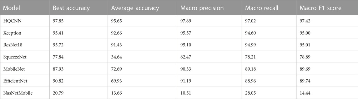
TABLE 5. Comparison of the HQCNN with other models.

Classification performance is often indicated by scalar values, such as accuracy, sensitivity, and specificity, among other different metrics Tiulpin et al. [6]. The confusion matrix is a more intuitive way to measure the model in the form of a matrix and also shows the classification of each category to achieve a more comprehensive measure. The confusion matrix, also known as the error matrix, is a standard format for representing accuracy evaluations and is represented in the form of a matrix with N rows and N columns, where N is the number of target classes. We can consider the confusion matrix as a summary table of the number of correct and incorrect predictions generated by the classification model for the classification task. We roughly measure the number of accurate classifications by looking at the diagonal values to determine the accuracy of the model. Figure 11 shows the confusion matrix of the prediction results of the HQCNN for the MRI dataset.

FIGURE 11

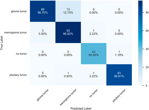
FIGURE 11. MRI confusion matrix.

5.2 Experiment2 OAI classification

The second phase of experiments targets the five classification problems for different types of knee osteoarthritis. The proposed integrated framework for OAI classification is trained according to the optimal hyperparameters of the HQCNN. We will analyze the advantages of quantum-to-classical transfer learning for OAI dataset classification in the following aspects. Figure 12 shows the training history before and after quantum-to-classical transfer, and Figure 13 shows the training history of connecting different classical models in the HQCNN model.

FIGURE 12

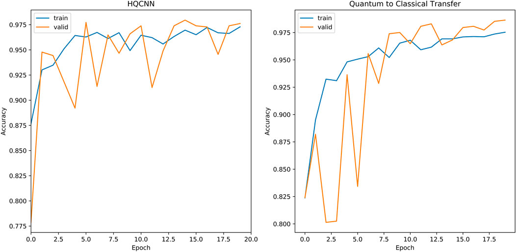
FIGURE 12. Training history before and after quantum-to-classical transfer.

FIGURE 13

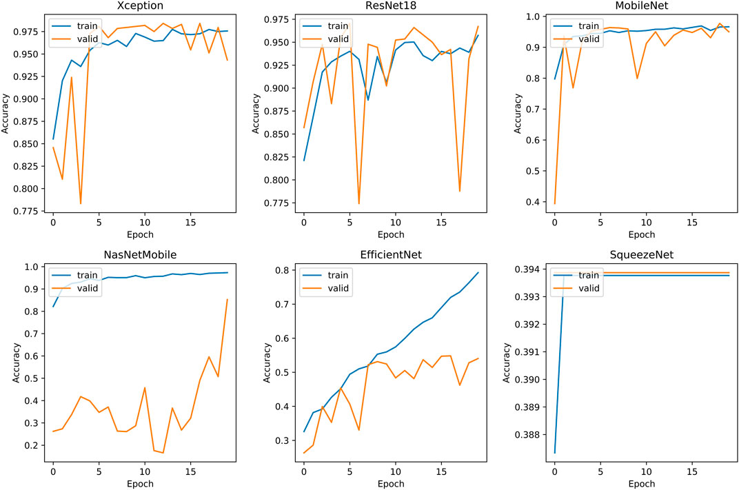
FIGURE 13. Training history of each model.

Validation accuracy fluctuations: SqueezeNet is the smoothest, but accuracy is always below 39%. EfficientNet is relatively stable, but accuracy is always below 56.38%. Xception has a decreasing trend after fluctuation at epoch = 4, the quantum classical to transfer learning method (QC) has fluctuation at epoch = 7, and it is relatively stable and increasing afterward. ResNet18 and NasNetMobile, in spite of the increasing validation set accuracy in general, have been experiencing large fluctuations and are obviously not stable.

Convergence speed: The accuracy curve can reflect the convergence speed of the loss function, the HQCNN is the best in convergence speed, and its accuracy exceeds 90% in less than two epochs.

Overfitting: SqueezeNet has serious overfitting, and NasNetMobile has good accuracy on the training set, but is far away from the validation set and test set, and has insufficient predictive power.

Figure 14 shows the confusion matrix of the prediction results of the HQCNN for the OAI dataset. Figure 15 shows the confusion matrix of QCTL’s prediction results for the OAI dataset, where the percentage in each square indicates the number of correct predictions for that class as a percentage of the total number of that class, that is, the accuracy of that class. The number above the percentage is the number of correct predictions for that class. We can see from the diagonal of this confusion matrix that the QCTL method can achieve 100% accuracy for the classification of OAI.

FIGURE 14

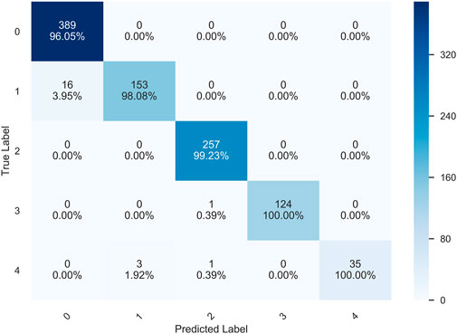
FIGURE 14. HQCNN confusion matrix.

FIGURE 15

FIGURE 15. QCTL confusion matrix.

In summary, the comparison experiments show that QCTL performs well in the OAI classification task, with the advantages of fast training speed, stable performance, and high classification accuracy, ranking first in accuracy, macro precision, macro recall, and macro f1 score metrics. The comparison results in Tables 6, 7 show that the method has the best average accuracy index of 98.36%. Therefore, the proposed method is more reliable for the classification of OAI.

TABLE 6

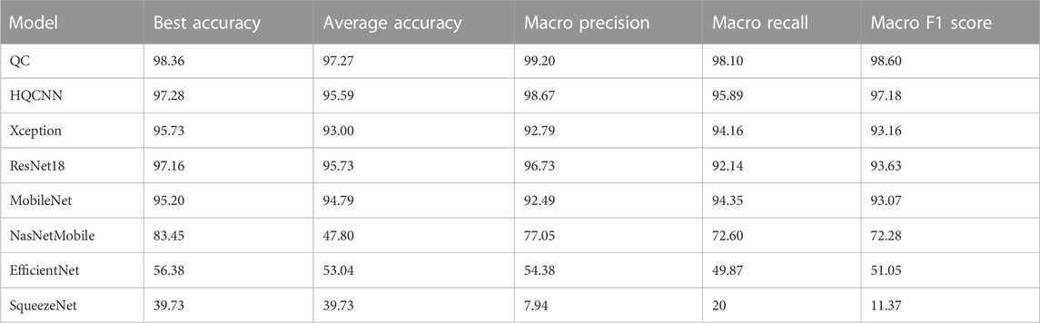
TABLE 6. Comparison of different classical models used in the HQCNN.

TABLE 7

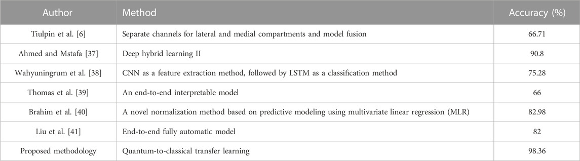
TABLE 7. Comparison of the proposed method for osteoarthritis of the knee with the prior art.

6 Conclusion

The salient concept of this work is to first design a HQCNN for MRI imaging of brain tumors to obtain a quantum convolutional network structure with stronger generalization capability. Next, quantum-to-classical transfer learning methods are used for hierarchical diagnosis of OAI images. In this paper, an improved HQCNN is proposed based on the quanvolutional neural networks proposed by Henderson et al. in Abohashima et al. [24]. In the comparison experiments, we uniformly used a 10-fold stratified sampling strategy to cross-validate the model and provide a comprehensive and detailed metric of network performance. The experimental results show that the improved HQCNN finally achieves 97.85% classification on the Brain Tumor MRI dataset. We update most or all parameters based on pre-trained weights. In feature extraction, the weights of the last layer (classifier) are trained using the coding characteristics of the pre-trained model. Using the trained model on the OAI dataset, quantum transfer learning finally achieved 98.36% classification on the OAI dataset. Future work will focus on combining different data point coding techniques to build deep hybrid networks for multi-class image classification Houssein et al. [34] and improve the extraction capability of the QCL. In summary, this study is an attempt of HQCNN in the medical field, and we should also think about how to use our method in practical applications in the medical field.

Data availability statement

Publicly available datasets were analyzed in this study. These data can be found here: https://www.kaggle.com/datasets/tommyngx/kneeoa https://www.kaggle.com/datasets/sartajbhuvaji/brain-tumor-classification-mri.

Author contributions

XC proposed the content and methods of the research and organized the database to conduct experiments and wrote the first draft. YF performed statistical analysis. YD provided direction for dissertation content. YZ and YT participated in the revision and reading of the manuscript. All authors contributed to the article and approved the submitted version.

Funding

This work was supported by the Open Fund of Advanced Cryptography and System Security Key Laboratory of Sichuan Province (Grant No. SKLACSS–202208) and National Natural Science Foundation of China (No.61772295).

Acknowledgments

The authors are grateful for the important technical help given by colleagues in the laboratory and the fund support.

Conflict of interest

YT was employed by ChongQing Promote Technologies Co. Ltd.

The remaining authors declare that the research was conducted in the absence of any commercial or financial relationships that could be construed as a potential conflict of interest.

Publisher’s note

All claims expressed in this article are solely those of the authors and do not necessarily represent those of their affiliated organizations, or those of the publisher, the editors, and the reviewers. Any product that may be evaluated in this article, or claim that may be made by its manufacturer, is not guaranteed or endorsed by the publisher.

References

1. Hunter DJ, March L, Chew M Osteoarthritis in 2020 and beyond: A lancet commission. The Lancet (2020) 396:1711–2. doi:10.1016/s0140-6736(20)32230-3

CrossRef Full Text | Google Scholar

2. Mobasheri A, Batt M An update on the pathophysiology of osteoarthritis. Ann Phys Rehabil Med (2016) 59:333–9. doi:10.1016/j.rehab.2016.07.004

PubMed Abstract | CrossRef Full Text | Google Scholar

3. Mathiessen A, Conaghan PG Synovitis in osteoarthritis: Current understanding with therapeutic implications. Arthritis Res Ther (2017) 19:18–9. doi:10.1186/s13075-017-1229-9

PubMed Abstract | CrossRef Full Text | Google Scholar

4. Baker K, McAlindon T Exercise for knee osteoarthritis. Curr Opin Rheumatol (2000) 12:456–63. doi:10.1097/00002281-200009000-00020

PubMed Abstract | CrossRef Full Text | Google Scholar

5. Kellgren JH, Lawrence J Radiological assessment of osteo-arthrosis. Ann Rheum Dis (1957) 16:494–502. doi:10.1136/ard.16.4.494

PubMed Abstract | CrossRef Full Text | Google Scholar

6. Tiulpin A, Thevenot J, Rahtu E, Lehenkari P, Saarakkala S Automatic knee osteoarthritis diagnosis from plain radiographs: A deep learning-based approach. Scientific Rep (2018) 8:1727–10. doi:10.1038/s41598-018-20132-7

CrossRef Full Text | Google Scholar

7. Simonyan K, Zisserman A Very deep convolutional networks for large-scale image recognition (2014). arXiv preprint arXiv:1409.1556.

Google Scholar

8. Antony J, McGuinness K, O’Connor NE, Moran K (2016). Quantifying radiographic knee osteoarthritis severity using deep convolutional neural networks. In 2016 23rd International Conference on Pattern Recognition (ICPR) (IEEE). 1195–200.

CrossRef Full Text | Google Scholar

9. Antony J, McGuinness K, Moran K, O’Connor NE (2017). Automatic detection of knee joints and quantification of knee osteoarthritis severity using convolutional neural networks. In Machine Learning and Data Mining in Pattern Recognition: 13th International Conference, MLDM 2017, New York, NY, USA, July 15-20, 2017, Proceedings 13 (Springer), 376–390

CrossRef Full Text | Google Scholar

10. Yang B, Lei Y, Liu J, Li W Social collaborative filtering by trust. IEEE Trans pattern Anal machine intelligence (2016) 39:1633–47. doi:10.1109/tpami.2016.2605085

CrossRef Full Text | Google Scholar

11. Swiecicki A, Li N, O’Donnell J, Said N, Yang J, Mather RC, et al. Deep learning-based algorithm for assessment of knee osteoarthritis severity in radiographs matches performance of radiologists. Comput Biol Med (2021) 133:104334. doi:10.1016/j.compbiomed.2021.104334

PubMed Abstract | CrossRef Full Text | Google Scholar

12. Zhang B, Tan J, Cho K, Chang G, Deniz CM Attention-based cnn for kl grade classification: Data from the osteoarthritis initiative. In: 2020 IEEE 17th international symposium on biomedical imaging (ISBI) (IEEE) (2020). p. 731–5.

CrossRef Full Text | Google Scholar

13. Bharti K, Cervera-Lierta A, Kyaw TH, Haug T, Alperin-Lea S, Anand A, et al. Noisy intermediate-scale quantum algorithms. Rev Mod Phys (2022) 94:015004. doi:10.1103/revmodphys.94.015004

CrossRef Full Text | Google Scholar

14. Landman J, Mathur N, Li YY, Strahm M, Kazdaghli S, Prakash A, et al. Quantum methods for neural networks and application to medical image classification. Quantum (2022) 6:881. doi:10.22331/q-2022-12-22-881

CrossRef Full Text | Google Scholar

15. Kiani BT, Villanyi A, Lloyd S Quantum medical imaging algorithms (2020). arXiv preprint arXiv:2004.02036.

Google Scholar

16. Azevedo V, Silva C, Dutra I Quantum transfer learning for breast cancer detection. Quan Machine Intelligence (2022) 4:5. doi:10.1007/s42484-022-00062-4

CrossRef Full Text | Google Scholar

17. Moradi S, Brandner C, Coggins M, Wille R, Drexler W, Papp L Error mitigation for quantum kernel based machine learning methods on ionq and ibm quantum computers (2022). arXiv preprint arXiv:2206.01573.

Google Scholar

18. Ahalya R, Snekhalatha U, Dhanraj V Automated segmentation and classification of hand thermal images in rheumatoid arthritis using machine learning algorithms: A comparison with quantum machine learning technique. J Therm Biol (2023) 111:103404. doi:10.1016/j.jtherbio.2022.103404

PubMed Abstract | CrossRef Full Text | Google Scholar

19. Shahwar T, Zafar J, Almogren A, Zafar H, Rehman AU, Shafiq M, et al. Automated detection of alzheimer’s via hybrid classical quantum neural networks. Electronics (2022) 11:721. doi:10.3390/electronics11050721

CrossRef Full Text | Google Scholar

20. Houssein EH, Abohashima Z, Elhoseny M, Mohamed WM Hybrid quantum-classical convolutional neural network model for Covid-19 prediction using chest x-ray images. J Comput Des Eng (2022) 9:343–63. doi:10.1093/jcde/qwac003

CrossRef Full Text | Google Scholar

21. Sengupta K, Srivastava PR Quantum algorithm for quicker clinical prognostic analysis: An application and experimental study using ct scan images of Covid-19 patients. BMC Med Inform Decis making (2021) 21:227–14. doi:10.1186/s12911-021-01588-6

CrossRef Full Text | Google Scholar

22. Bergholm V, Izaac J, Schuld M, Gogolin C, Ahmed S, Ajith V, et al. Pennylane: Automatic differentiation of hybrid quantum-classical computations (2018). arXiv preprint arXiv:1811.04968.

Google Scholar

23. Henderson M, Shakya S, Pradhan S, Cook T Quanvolutional neural networks: Powering image recognition with quantum circuits. Quan Machine Intelligence (2020) 2:2. doi:10.1007/s42484-020-00012-y

CrossRef Full Text | Google Scholar

24. Abohashima Z, Elhosen M, Houssein EH, Mohamed WM Classification with quantum machine learning: A survey (2020). arXiv preprint arXiv:2006.12270.

Google Scholar

25. Schuld M Supervised quantum machine learning models are kernel methods (2021). arXiv preprint arXiv:2101.11020.

Google Scholar

26. Havlíček V, Córcoles AD, Temme K, Harrow AW, Kandala A, Chow JM, et al. Supervised learning with quantum-enhanced feature spaces. Nature (2019) 567:209–12. doi:10.1038/s41586-019-0980-2

PubMed Abstract | CrossRef Full Text | Google Scholar

27. Huang H-Y, Broughton M, Mohseni M, Babbush R, Boixo S, Neven H, et al. Power of data in quantum machine learning. Nat Commun (2021) 12:2631. doi:10.1038/s41467-021-22539-9

PubMed Abstract | CrossRef Full Text | Google Scholar

28. Mari A, Bromley TR, Izaac J, Schuld M, Killoran N Transfer learning in hybrid classical-quantum neural networks. Quantum (2020) 4:340. doi:10.22331/q-2020-10-09-340

CrossRef Full Text | Google Scholar

29. Latorre JI Image compression and entanglement (2005). arXiv preprint quant-ph/0510031.

Google Scholar

30. Le PQ, Dong F, Hirota K A flexible representation of quantum images for polynomial preparation, image compression, and processing operations. Quan Inf Process (2011) 10:63–84. doi:10.1007/s11128-010-0177-y

CrossRef Full Text | Google Scholar

31. Chen P Knee osteoarthritis severity grading dataset. Mendeley Data (2018) 1. doi:10.17632/56rmx5bjcr.1

CrossRef Full Text | Google Scholar

32. Quinonero-Candela J, Sugiyama M, Schwaighofer A, Lawrence ND Dataset shift in machine learning. Mit Press (2008).

Google Scholar

33. Glorot X, Bengio Y Understanding the difficulty of training deep feedforward neural networks. In: Proceedings of the thirteenth international conference on artificial intelligence and statistics (JMLR Workshop and Conference Proceedings) (2010). p. 249–56.

Google Scholar

34. Houssein E, Abohashima Z, Elhoseny M, Mohamed M (2021). Hybrid quantum convolutional neural networks model for covid-19 prediction using chest x-ray images.

Google Scholar

35. Deng J, Dong W, Socher R, Li L-J, Li K, Fei-Fei L (2009). Imagenet: A large-scale hierarchical image database. In 2009 IEEE conference on computer vision and pattern recognition (Ieee), 248–55.

CrossRef Full Text | Google Scholar

36. Venegas-Andraca SE. Discrete quantum walks and quantum image processing (2005).

Google Scholar

37. Ahmed SM, Mstafa RJ Identifying severity grading of knee osteoarthritis from x-ray images using an efficient mixture of deep learning and machine learning models. Diagnostics (2022) 12:2939. doi:10.3390/diagnostics12122939

PubMed Abstract | CrossRef Full Text | Google Scholar

38. Wahyuningrum RT, Anifah L, Purnama IKE, Purnomo MH (2019). A new approach to classify knee osteoarthritis severity from radiographic images based on cnn-lstm method. In 2019 IEEE 10th International Conference on Awareness Science and Technology (iCAST) (IEEE), 1–6.

CrossRef Full Text | Google Scholar

39. Thomas KA, Kidziński Ł, Halilaj E, Fleming SL, Venkataraman GR, Oei EH, et al. Automated classification of radiographic knee osteoarthritis severity using deep neural networks. Radiol Artif Intelligence (2020) 2:e190065. doi:10.1148/ryai.2020190065

CrossRef Full Text | Google Scholar

40. Brahim A, Jennane R, Riad R, Janvier T, Khedher L, Toumi H, et al. A decision support tool for early detection of knee osteoarthritis using x-ray imaging and machine learning: Data from the osteoarthritis initiative. Comput Med Imaging Graphics (2019) 73:11–8. doi:10.1016/j.compmedimag.2019.01.007

CrossRef Full Text | Google Scholar

41. Liu B, Luo J, Huang H Toward automatic quantification of knee osteoarthritis severity using improved faster r-cnn. Int J Comput Assist Radiol Surg (2020) 15:457–66. doi:10.1007/s11548-019-02096-9

PubMed Abstract | CrossRef Full Text | Google Scholar