Atomic magnetometers and their application in industry

In modern detection techniques, high-precision magnetic field detection plays a crucial role. Atomic magnetometers stand out among other devices due to their high sensitivity, large detection range, low power consumption, high sampling rate, continuous gradient measurements, and good confidentiality. Atomic magnetometers have become a hot topic in the field of magnetometry due to their ability to measure not only the total strength of the Earth’s magnetic field, but also its gradients, both slow- and high-velocity transient magnetic fields, both strong and weak. In recent years, researchers have shifted their focus from improving the performance of atomic magnetometers to utilizing their exceptional capabilities for practical applications. The objective of this study is to explore the measurement principle and detection method of atomic magnetometers, and it also examines the technological means and research progress of atomic magnetometers in various industrial fields, including magnetic imaging, material examination, underwater magnetic target detection, and magnetic communication. Additionally, this study discusses the potential applications and future development trends of atomic magnetometers.

1 Introduction

The magnetic field is one of the earliest physical phenomena recognized by humans. Looking back at the history of electromagnetic theory, people have been studying magnetic fields scientifically for hundreds of years, ever since Danish physicist Hans Christian Ørsted discovered magnetic effect of electric current in the 1820s. Measuring the magnetic field will help one better understand the physical information contained in magnetic phenomena. As a result, magnetic field detection has become an essential means of studying physical phenomena related to magnetic objects. At present, the related research on the detection of weak magnetic fields has been widely used in various fields such as geology [1–3], aeromagnetic investigation [4–6], medical [7–9], and military studies [10–12]. With the improvement of science and technology, people’s research on magnetic fields has become more detailed, and the measurement of weak magnetic fields has played a role in more and more fields, ranging from planetary universes to small molecules and atoms, in which weak magnetic detection plays a crucial role.

The core component of weak magnetic detection is the magnetic field sensors. At present, the instruments that can measure weak magnetic fields mainly include fluxgate sensors [13–15], superconducting quantum interference magnetometers (SQUID) [16–18], proton magnetometers [19–21], Hall magnetic sensors [22–24], Tunnel Magneto-Resistance sensors (TMR) [25–27], and atomic magnetometers [28–30]. The sensitivity of the fluxgate magnetometer can reach at ∼ nT level [31], which is challenging to apply when more precise measurements are required; the Superconducting Quantum Interference Device (SQUID), although highly sensitive, requires low temperature cooling, and high production and operating costs [32]; the proton magnetometer is a high-precision device for weak magnetostatic field measurement with high stability and is widely used, but it has higher power consumption [33]; Hall magnetic sensors are small in size, low cost, but the detection capability can only reach 10 nT level [34]; the TMR sensor can reach a resolution of several pT at the excitation frequency, however, its preparation process is relatively complicated [35]; the atomic magnetometer is a magnetometer with ultra-high sensitivity developed in the past 10 years, and it is also the most cutting-edge research direction in the field of weak magnetic field measurement in the world, its sensitivity can reach the fT level like SQUID, and compared with SQUID, its structure is considerably simplified, and it does not require cryogenic cooling [36]. Based on the above advantages, it can be said that it is a magnetometer instrument with excellent performance. Table 1 summarizes several representative and commercialized magnetic field sensors, and compares their parameters and performance.

TABLE 1

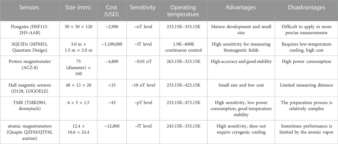
TABLE 1. Different instruments to measure weak magnetic field.

The atomic magnetometer is a magnetometer with ultra-high sensitivity that has been developed in the last decade. The working materials of the atomic magnetometer mainly include three alkali metals such as potassium, rubidium, and cesium (K, Rb, and Cs). This is because there is only one unpaired electron in the outermost layer of the alkali metal atom, which can easily produce atomic polarization by optical pumping. In terms of working mechanism, atomic magnetometers mainly include Coherent Population Trapping (CPT), Nonlinear Magneto-Optical Rotation (NMOR), and Spin-Exchange-Relaxtion-Free (SERF). To date, several studies have been carried out. The CPT phenomenon was first discovered by Scully and Fleischhauer in 1992 [37]. In 1998, Nagel et al. developed the first cesium-atom CPT magnetometer to measure alternating magnetic fields [38]. In 2000, Budker et al. developed a nonlinear magneto-optical rotation (NMOR) magnetometer operated at room temperature and showed that its sensitivity based on the photon scattering noise limit could reach 0.3 fT/Hz^1/2 near zero magnetic fields [39]. Because of the narrow resonances of NMOR, NMOR was rapidly applied to highly sensitive magnetometers. Using frequency modulation scheme, NMOR magnetometer can also work under geomagnetic field, with sensitivity up to 60 fT/Hz^1/2 [40]. The SERF atomic magnetometer was first proposed in 2002. The Romalis group published an article entitled “High Sensitivity Atomic Magnetometer without Spin Exchange Relaxation Free (SERF),” in which they reported a SERF magnetometer whose magnetic sensitivity could reach 10 fT/Hz^1/2 [41]. The following year, the group reported a further optimized potassium atomic magnetometer based on the SERF mechanism, with a sensitivity of 0.54 fT/Hz^1/2, and the expected theoretical sensitivity could reach 1 aT/Hz^1/2, surpassing the superconductor’s highest sensitivity ever [42].

Extensive overviews of atomic magnetometers have been previously performed by Murzin et al. in 2020 [43], Bennett et al. in 2021 [44], Liu et al. in 2022 [45], and Aslam et al. in 2023 [46], detailing atomic magnetometers for biomedical applications, aerospace applications, and traditional magnetoencephalography (MEG) systems in medicine. The difference with them is that this review focuses on the development and application of atomic magnetometers in industry. With the increasing miniaturization and sensitivity of atomic magnetometers, they are used in many industrial applications, such as magnetic imaging, battery testing, underwater target detection and localization, and magnetic communication. The application of atomic magnetometers in these fields can provide contact-free magnetic field measurements for safety inspections, battery research, and other related research directions.

The atomic magnetometer is one of the most sensitive magnetic measuring equipment at present. On the one hand, its advantages of high sensitivity, non-low temperature operation and miniaturization will enable it to be used in more fields. On the other hand, the improvement of magnetometer performance has been driven by the requirements of its application field. Researchers have been developing atomic magnetometers with higher sensitivity according to the needs of practical applications. This interaction has greatly promoted the development of atomic magnetometers in device development and practical application. Nowadays, the measurement of weak magnetic field based on atomic magnetometers has been used more and more widely in industry.

2 Theoretical basis of an all-optical atomic magnetometer

The atomic magnetometer reflects the magnitude of the magnetic field by measuring the Larmor precession frequency of the polarization vector of the atomic spin in the external magnetic field. Since there is only one unpaired electron in the outermost layer of an alkali metal atom, the total spin of the atom is equal to the vector sum of the nuclear spin and the valence electron spin, and the spin of the outermost single electron can be easily manipulated by optical pumping and other methods. As a result, atomic magnetometers all choose alkali metal atoms as working substances. Conventional atomic magnetometers adopt the radio frequency field modulation scheme and direct detection of light intensity, however, at high temperatures, the detection light is diverted from the atomic resonance line and the birefringence effect of the medium is used to detect the magnetic field.

In Figure 1, there is how an atomic magnetometer operates, taking a cesium atomic magnetometer as an example: First, a circularly polarized pump light beam polarizes atoms in the direction of the pump light. Under the action of an external magnetic field, the spin polarization vector of the atom will do Larmor precession around the magnetic field.

FIGURE 1

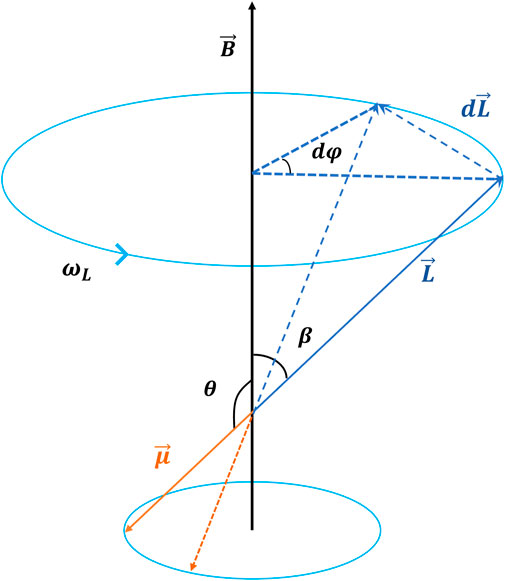
FIGURE 1. Larmor progression of the atomic magnetic moment in a magnetic field.

The atomic magnetic moment is not subjected to a force in a uniform external magnetic field but is acted by a moment. The torque of the magnetic field on the atomic magnetic moment is:

$\begin{array}{c}\overrightarrow{\mathrm{\tau }}=\overrightarrow{\mathrm{\mu }}\times \overrightarrow{\mathrm{B}}\end{array}(1)$

Where $\overrightarrow{\mathrm{\mu }}$ is the atomic magnetic moment; $\overrightarrow{\mathrm{B}}$ is the external magnetic field; $\overrightarrow{\mathrm{\tau }}$ is the torque applied to the atomic magnetic moment.

And the existence of a moment will cause the change in angular momentum:

$\begin{array}{c}\frac{\mathrm{d}\overrightarrow{\mathrm{L}}}{\mathrm{d}\mathrm{t}}=\overrightarrow{\mathrm{\tau }}\end{array}(2)$

$\overrightarrow{\mathrm{L}}$ is the moment of force.

Let the angle between the angular momentum and the direction of the magnetic field be $\mathrm{\beta }$, and when the time interval is $\mathrm{d}\mathrm{t}$, the precession angle of the angular momentum is $\mathrm{d}\mathrm{\phi }$, then the change in angular momentum is:

$\begin{array}{c}\mathrm{d}\mathrm{L}=\mathrm{L}\mathrm{s}\mathrm{i}\mathrm{n}\mathrm{\beta }\mathrm{d}\mathrm{\phi }\end{array}(3)$

Therefore

$\begin{array}{c}\frac{\mathrm{d}\mathrm{L}}{\mathrm{d}\mathrm{t}}=\mathrm{L}\mathrm{s}\mathrm{i}\mathrm{n}\mathrm{\beta }\frac{\mathrm{d}\mathrm{\phi }}{\mathrm{d}\mathrm{t}}=\mathrm{L}\mathrm{s}\mathrm{i}\mathrm{n}\mathrm{\beta }{\mathrm{\omega }}_{\mathrm{L}}\end{array}(4)$

Where ${\mathrm{\omega }}_{\mathrm{L}}=\frac{\mathrm{d}\mathrm{\phi }}{\mathrm{d}\mathrm{t}}$ is the angular velocity of the precession of the atomic magnetic moment around the magnetic field.

Let the angle between the magnetic moment and the direction of the magnetic field be $\mathrm{\theta }$, then:

$\mathrm{\tau }=\mathrm{\mu }\mathrm{B}\mathrm{s}\mathrm{i}\mathrm{n}\mathrm{\theta }$

$\begin{array}{c}\mathrm{L}\sin \mathrm{\beta }{\mathrm{\omega }}_{\mathrm{L}}=\mathrm{\mu }\mathrm{B}\mathrm{s}\mathrm{i}\mathrm{n}\mathrm{\theta }\end{array}(5)$

Where $\mathrm{\mu }$ is the value of the atomic magnetic moment in Eq. 1. The angular velocity of Larmor’s precession is:

$\begin{array}{c}{\mathrm{\omega }}_{\mathrm{L}}=\frac{\mathrm{\mu }}{\mathrm{L}}\mathrm{B}=\mathrm{\gamma }\mathrm{B}\end{array}(6)$

Where $\mathrm{\gamma }$ is the gyromagnetic ratio. Eq. 6 is the angular velocity formula of Larmor precession.

As shown in Figure 2, the atomic magnetometer first utilizes a beam of circularly polarized pump light to polarize the atoms along the direction of the pump light. Under the action of an external magnetic field, the spin polarization vector of the atom will do Larmor precession around the magnetic field. A linearly polarized light is used in a direction perpendicular to the pump light to detect the projection of the polarization vector in the direction of the detection light. The polarized atoms have contrasting refractive indices for the left- and right-handed components of linearly polarized light, resulting in a slight deflection in the plane of polarization of the linearly polarized light passing through the atomic gas cell. When the modulation frequency of the pump light resonates with the Larmor precession frequency, the deflection angle of the detection light is the largest. Consequently, by judging the modulation frequency corresponding to the maximum deflection angle, the magnitude of the external magnetic field can be measured [47].

FIGURE 2

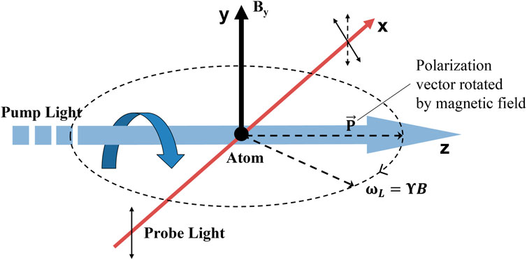
FIGURE 2. Schematic diagram of the working principle of the alkali metal atomic magnetometer.

Quantum mechanics sets fundamental limits on the best sensitivity that can be achieved in an atomic magnetometer. Project noise is one of the limits. That’s because if an atom is polarized in a particular direction, a random result will be produced when the angular momentum projection m is measured in the orthogonal direction. When the factors of order unity that depend on particulars of the system are ignored, the sensitivity of a magnetic-field measurement performed for a time $\mathrm{T}$ with an ensemble of $\mathrm{N}$ atoms with coherence time $\mathrm{\tau }$ is [29]:

$\begin{array}{c}\mathrm{\delta }\mathrm{B}\cong \frac{1}{\mathrm{g}{\mathrm{\mu }}_{\mathrm{B}}}\frac{\mathit{\hslash }}{\sqrt{\mathrm{N}\mathrm{\tau }\mathrm{T}}}\end{array}(7)$

Where ${\mathrm{\mu }}_{\mathrm{B}}$ is the Bohr magneton, $\mathrm{g}$ is the ground-state Landé factor, and $\mathrm{\hslash }$ is Planck’s constant. In addition, there is also photon shot noise, which can be described by the following equation:

$\begin{array}{c}\mathrm{\delta }{\mathrm{\phi }}_{\mathrm{s}}\cong \frac{1}{2\sqrt{{\dot{\mathrm{N}}}_{\mathrm{p}\mathrm{h}}\mathrm{T}}}\end{array}(8)$

Where ${\dot{\mathrm{N}}}_{\mathrm{p}\mathrm{h}}$ is the probe-photon flux (in photons per second) behind the atomic sample.

3 Method: weak magnetic detection

The geomagnetic field serves as the background field for weak magnetic detection. There will be magnetic anomalies in the geomagnetic field when ferromagnetic objects are present, and then the position and magnetic moment of the ferromagnetic object can be found by detecting this anomaly.

Assuming that a magnetic dipole is in a magnetic field, its magnetic moment is expressed as $\overrightarrow{\mathrm{p}}$, and $\overrightarrow{\mathrm{r}}$ is its position vector, then its magnetic flux density at $\overrightarrow{\mathrm{r}}$ is [48]

$\begin{array}{c}\overrightarrow{\mathrm{B}}=\frac{{\mathrm{\mu }}_0}{4\mathrm{\pi }}\frac{3\left(\overrightarrow{\mathrm{p}}\bullet \overrightarrow{\mathrm{n}}\right)\overrightarrow{\mathrm{n}}-\overrightarrow{\mathrm{p}}}{{\mathrm{r}}^3}\end{array}(9)$

Where ${\mathrm{\mu }}_0=4\mathrm{\pi }\times {10}^{-7}\mathrm{H}/\mathrm{m}$ is the permeability of vacuum, $\mathrm{r}=\left|\overrightarrow{\mathrm{r}}\right|$ is the distance from the origin to the measurement point, and $\overrightarrow{\mathrm{n}}=\frac{\overrightarrow{\mathrm{r}}}{\left|\mathrm{r}\right|}$ is the unit vector.

The magnetic field at the point $\mathrm{d}\mathrm{r}$ from the measurement point is:

$\begin{array}{c}\overrightarrow{{\mathrm{B}}^{\prime }}=\frac{{\mathrm{\mu }}_0}{4\mathrm{\pi }}\frac{3\left(\overrightarrow{\mathrm{p}}\bullet \overrightarrow{\mathrm{n}}\right)\overrightarrow{\mathrm{n}}-\overrightarrow{\mathrm{p}}}{{\left(\mathrm{r}+\mathrm{d}\mathrm{r}\right)}^3}\\ \overrightarrow{{\mathrm{B}}^{\prime }}-\overrightarrow{\mathrm{B}}=\frac{{\mathrm{\mu }}_0}{4\mathrm{\pi }}\left(3\left(\overrightarrow{\mathrm{p}}\bullet \overrightarrow{\mathrm{n}}\right)\overrightarrow{\mathrm{n}}-\overrightarrow{\mathrm{p}}\right)\left(\frac{\partial }{\partial \mathrm{r}}\frac{1}{{\mathrm{r}}^3}\mathrm{d}\mathrm{r}\right)\\ =-\frac{3}{\mathrm{r}}\frac{{\mathrm{\mu }}_0}{4\mathrm{\pi }}\frac{3\left(\overrightarrow{\mathrm{p}}\bullet \overrightarrow{\mathrm{n}}\right)\overrightarrow{\mathrm{n}}-\overrightarrow{\mathrm{p}}}{{\mathrm{r}}^3}\mathrm{d}\mathrm{r}=-\frac{3}{\mathrm{r}}\overrightarrow{\mathrm{B}}\mathrm{d}\mathrm{r}\end{array}(10)$

Express the vector difference in terms of the magnetic field gradient as

$\begin{array}{c}\overrightarrow{{\mathrm{B}}^{\prime }}-\overrightarrow{\mathrm{B}}=\left(\begin{array}{c}\nabla {\mathrm{B}}_{\mathrm{x}}\bullet \overrightarrow{\mathrm{n}}\mathrm{d}\mathrm{r}\\ \nabla {\mathrm{B}}_{\mathrm{y}}\bullet \overrightarrow{\mathrm{n}}\mathrm{d}\mathrm{r}\\ \nabla {\mathrm{B}}_{\mathrm{z}}\bullet \overrightarrow{\mathrm{n}}\mathrm{d}\mathrm{r}\end{array}\right)\\ =\left(\begin{array}{c}{\partial }_{\mathrm{x}}{\mathrm{B}}_{\mathrm{x}}{\partial }_{\mathrm{y}}{\mathrm{B}}_{\mathrm{x}}{\partial }_{\mathrm{z}}{\mathrm{B}}_{\mathrm{x}}\\ {\partial }_{\mathrm{x}}{\mathrm{B}}_{\mathrm{y}}{\partial }_{\mathrm{y}}{\mathrm{B}}_{\mathrm{y}}{\partial }_{\mathrm{z}}{\mathrm{B}}_{\mathrm{y}}\\ {\partial }_{\mathrm{x}}{\mathrm{B}}_{\mathrm{z}}{\partial }_{\mathrm{y}}{\mathrm{B}}_{\mathrm{z}}{\partial }_{\mathrm{z}}{\mathrm{B}}_{\mathrm{z}}\end{array}\right)\overrightarrow{\mathrm{n}}\mathrm{d}\mathrm{r}\end{array}(11)$

Let

$\begin{array}{c}\mathbf{G}\equiv \left(\begin{array}{c}{\partial }_{\mathrm{x}}{\mathrm{B}}_{\mathrm{x}}{\partial }_{\mathrm{y}}{\mathrm{B}}_{\mathrm{x}}{\partial }_{\mathrm{z}}{\mathrm{B}}_{\mathrm{x}}\\ {\partial }_{\mathrm{x}}{\mathrm{B}}_{\mathrm{y}}{\partial }_{\mathrm{y}}{\mathrm{B}}_{\mathrm{y}}{\partial }_{\mathrm{z}}{\mathrm{B}}_{\mathrm{y}}\\ {\partial }_{\mathrm{x}}{\mathrm{B}}_{\mathrm{z}}{\partial }_{\mathrm{y}}{\mathrm{B}}_{\mathrm{z}}{\partial }_{\mathrm{z}}{\mathrm{B}}_{\mathrm{z}}\end{array}\right)\end{array}(12)$

From Eqs 10, 11 we can derive that

$\begin{array}{c}\left(\begin{array}{c}{\partial }_{\mathrm{x}}{\mathrm{B}}_{\mathrm{x}}{\partial }_{\mathrm{y}}{\mathrm{B}}_{\mathrm{x}}{\partial }_{\mathrm{z}}{\mathrm{B}}_{\mathrm{x}}\\ {\partial }_{\mathrm{x}}{\mathrm{B}}_{\mathrm{y}}{\partial }_{\mathrm{y}}{\mathrm{B}}_{\mathrm{y}}{\partial }_{\mathrm{z}}{\mathrm{B}}_{\mathrm{y}}\\ {\partial }_{\mathrm{x}}{\mathrm{B}}_{\mathrm{z}}{\partial }_{\mathrm{y}}{\mathrm{B}}_{\mathrm{z}}{\partial }_{\mathrm{z}}{\mathrm{B}}_{\mathrm{z}}\end{array}\right)\overrightarrow{\mathrm{n}}=-\frac{3}{\mathrm{r}}\overrightarrow{\mathrm{B}}=\mathbf{G}\overrightarrow{\mathrm{n}}\end{array}(13)$

Then, $\overrightarrow{\mathrm{r}}=\mathrm{r}\overrightarrow{\mathrm{n}}$ can be expressed as:

$\begin{array}{c}\overrightarrow{\mathrm{r}}=-3{\mathbf{G}}^{-1}\overrightarrow{\mathrm{B}}=-3{\left(\begin{array}{c}{\partial }_{\mathrm{x}}{\mathrm{B}}_{\mathrm{x}}{\partial }_{\mathrm{y}}{\mathrm{B}}_{\mathrm{x}}{\partial }_{\mathrm{z}}{\mathrm{B}}_{\mathrm{x}}\\ {\partial }_{\mathrm{x}}{\mathrm{B}}_{\mathrm{y}}{\partial }_{\mathrm{y}}{\mathrm{B}}_{\mathrm{y}}{\partial }_{\mathrm{z}}{\mathrm{B}}_{\mathrm{y}}\\ {\partial }_{\mathrm{x}}{\mathrm{B}}_{\mathrm{z}}{\partial }_{\mathrm{y}}{\mathrm{B}}_{\mathrm{z}}{\partial }_{\mathrm{z}}{\mathrm{B}}_{\mathrm{z}}\end{array}\right)}^{-1}\left(\begin{array}{c}{\mathrm{B}}_{\mathrm{x}}\\ {\mathrm{B}}_{\mathrm{y}}\\ {\mathrm{B}}_{\mathrm{z}}\end{array}\right)\end{array}(14)$

In the positioning of magnetic target, the target can be equivalent to the magnetic dipole model because the position of the magnetometer is often far away from the position of the target. In the measurement, the external magnetic field is usually the geomagnetic field. The following will analyze the case when the external magnetic field is the geomagnetic field. In the spatial rectangular coordinate system, the $\mathrm{x}$ direction represents the geographical east direction, the $\mathrm{y}$ direction represents the geographical north direction, and the $\mathrm{z}$ direction is vertically downward. The position of the magnetic target is $\left({\mathrm{x}}_0,{\mathrm{y}}_0,{\mathrm{z}}_0\right)$, then the magnetic field at $\left(\mathrm{x},\mathrm{y},\mathrm{z}\right)$ is [49]:

$\overrightarrow{\mathrm{B}}={\mathrm{B}}_{\mathrm{x}}{\overrightarrow{\mathrm{e}}}_{\mathrm{x}}+{\mathrm{B}}_{\mathrm{y}}{\overrightarrow{\mathrm{e}}}_{\mathrm{y}}+{\mathrm{B}}_{\mathrm{z}}{\overrightarrow{\mathrm{e}}}_{\mathrm{z}}$

${\mathrm{B}}_{\mathrm{x}}=\frac{{\mathrm{\mu }}_0{\mathrm{p}}_0}{4\mathrm{\pi }}\frac{{\mathrm{r}}^2\mathrm{l}-3{\mathrm{r}}_{\mathrm{x}}\left({\mathrm{r}}_{\mathrm{x}}\mathrm{l}+{\mathrm{r}}_{\mathrm{y}}\mathrm{m}-{\mathrm{z}}_0\mathrm{n}\right)}{{\mathrm{r}}^5}$

${\mathrm{B}}_{\mathrm{y}}=\frac{{\mathrm{\mu }}_0{\mathrm{p}}_0}{4\mathrm{\pi }}\frac{{\mathrm{r}}^2\mathrm{m}-3{\mathrm{r}}_{\mathrm{y}}\left({\mathrm{r}}_{\mathrm{x}}\mathrm{l}+{\mathrm{r}}_{\mathrm{y}}\mathrm{m}-{\mathrm{z}}_0\mathrm{n}\right)}{{\mathrm{r}}^5}$

$\begin{array}{c}{\mathrm{B}}_{\mathrm{z}}=\frac{{\mathrm{\mu }}_0{\mathrm{p}}_0}{4\mathrm{\pi }}\frac{{\mathrm{r}}^2\mathrm{n}-3{\mathrm{z}}_0\left({\mathrm{r}}_{\mathrm{x}}\mathrm{l}+{\mathrm{r}}_{\mathrm{y}}\mathrm{m}-{\mathrm{z}}_0\mathrm{n}\right)}{{\mathrm{r}}^5}\end{array}(15)$

$\begin{array}{c}\mathrm{r}=\sqrt{{\mathrm{r}}_{\mathrm{x}}^2+{\mathrm{r}}_{\mathrm{y}}^2+{\mathrm{r}}_{\mathrm{z}}^2}\end{array}(16)$

Among them:

$\begin{array}{c}\left\{\begin{array}{c}{\mathrm{r}}_{\mathrm{x}}=\mathrm{x}-{\mathrm{x}}_0\\ {\mathrm{r}}_{\mathrm{y}}=\mathrm{y}-{\mathrm{y}}_0\\ {\mathrm{r}}_{\mathrm{z}}=\mathrm{z}-{\mathrm{z}}_0\end{array}\right.\end{array}(17)$

$\begin{array}{c}\left\{\begin{array}{c}\mathrm{l}=\mathrm{c}\mathrm{o}\mathrm{s}\mathrm{I}\mathrm{c}\mathrm{o}\mathrm{s}\mathrm{D}\\ \mathrm{m}=\mathrm{c}\mathrm{o}\mathrm{s}\mathrm{I}\mathrm{s}\mathrm{i}\mathrm{n}\mathrm{D}\\ \mathrm{n}=\mathrm{s}\mathrm{i}\mathrm{n}\mathrm{I}\end{array}\right.\end{array}(18)$

Where ${\overrightarrow{\mathrm{e}}}_{\mathrm{x}}$, ${\overrightarrow{\mathrm{e}}}_{\mathrm{y}}$ and ${\overrightarrow{\mathrm{e}}}_{\mathrm{z}}$ are unit vectors, ${\mathrm{p}}_0$ is the magnetic moment of the magnetic target, $\mathrm{r}$ is the distance between the detection point and the magnetic target, ${\mathrm{r}}_{\mathrm{x}}$, ${\mathrm{r}}_{\mathrm{y}}$, and ${\mathrm{r}}_{\mathrm{z}}$ are the components of $\mathrm{r}$ in the x, y, and z directions, $\mathrm{I}$ and $\mathrm{D}$ represent the magnetic dip and magnetic declination of the geomagnetic field.

Weak magnetic field detection belongs to the category of weak signal detection. The term “weak” does not only refer to the small amplitude of the signal, but also to the small size of the signal about the noise. The magnetic field is a space vector, and the magnetic signal contains a wealth of information about its spatial distribution and even its rate of change. In the detection of weak magnetic fields, depending on the mode of operation of the magnetometer, there are magnetic field scalar measurements [50], magnetic field vector measurements [51], and full-tensor magnetic field gradient measurements [52].

(1) Magnetic field scalar measurement

The magnetic field scalar measurement method generally applies instruments such as proton magnetometers and light-pumped atomic magnetometers to measure the total magnetic field to be measured, and from the measured magnetic field information, further information such as the position of the target object can be obtained. In addition, essential system calibration and calibration of vector magnetometer systems are frequently performed using magnetic field scalar measurements.

(2) Magnetic field vector measurement

A single magnetic field component of a geomagnetic field or magnetic target is measured using vector magnetic sensors in a vector magnetic field detection system. Compared with scalar magnetic field detection, applications based on magnetic field vector detection provide more information by measuring the characteristics and patterns of magnetic field vector distribution in space and are particularly widespread in military applications. Otnes proposed object detecting method which combined noise suppression in 3-axial magnetic measurements in 2007 [53]. By using this method, a decision variable with an SNR of 20 dB from an input signal could be extracted. They also proposed a block-based adaptive procedure. It has proved to have good performance with a detection delay of 85 s in the actual test. In the same year, Hu et al. placed tiny magnetic objects in the human body and measured the position and pointing of the magnets through a magnetic field vector sensor installed at a fixed location to track magnetic objects in the human body [54]. The linear algorithm is applied to the actual positioning system. The simulation and experimental results show that satisfactory tracking accuracy can be obtained by using enough triaxial magnetic sensor arrays.

(3) The full magnetic gradient tensor (MGT)

Full tensor magnetic field gradient measurement is a method of measuring the spatial rate of change of the three components of the magnetic field for magnetometers [55]. The magnetic detection system realized by using the magnetic gradient tensor has the characteristics of strong anti-interference ability and large amount of information in magnetic measurement, so it is often used for magnetic target detection and position positioning. When detecting magnetic anomalies, a single vector magnetometer can only obtain the information of the three components of the magnetic anomaly but cannot obtain the information of the gradient tensor of the magnetic field. Therefore, it is necessary to use multiple three-component magnetometers to form the magnetic gradient tensor measurement system. In a common MGT system, seven magnetometers are formed into three orthogonal axis arrays, with three magnetometers on each array. Three magnetometers on three axes respectively measure the magnetic field change rate of the axis, and then the magnetic gradient tensor information can be obtained.

From the definition of tensor gradient and the definition of the magnetic field at any point (x, y, z) in Eq. 15, the gradient tensor $\mathbf{G}$ of the magnetic dipole field is given by the following equation.

$\begin{array}{c}\mathbf{G}=\left(\begin{array}{c}\frac{{\partial \mathrm{B}}_{\mathrm{x}}}{\partial \mathrm{x}}\frac{{\partial \mathrm{B}}_{\mathrm{y}}}{\partial \mathrm{x}}\frac{{\partial \mathrm{B}}_{\mathrm{z}}}{\partial \mathrm{x}}\\ \frac{{\partial \mathrm{B}}_{\mathrm{x}}}{\partial \mathrm{y}}\frac{{\partial \mathrm{B}}_{\mathrm{y}}}{\partial \mathrm{y}}\frac{{\partial \mathrm{B}}_{\mathrm{z}}}{\partial \mathrm{y}}\\ \frac{{\partial \mathrm{B}}_{\mathrm{x}}}{\partial \mathrm{z}}\frac{{\partial \mathrm{B}}_{\mathrm{y}}}{\partial \mathrm{z}}\frac{{\partial \mathrm{B}}_{\mathrm{z}}}{\partial \mathrm{z}}\end{array}\right)\\ =\left(\begin{array}{c}{\mathrm{B}}_{\mathrm{x}\mathrm{x}}{\mathrm{B}}_{\mathrm{y}\mathrm{x}}{\mathrm{B}}_{\mathrm{z}\mathrm{x}}\\ {\mathrm{B}}_{\mathrm{x}\mathrm{y}}{\mathrm{B}}_{\mathrm{y}\mathrm{y}}{\mathrm{B}}_{\mathrm{z}\mathrm{y}}\\ {\mathrm{B}}_{\mathrm{x}\mathrm{z}}{\mathrm{B}}_{\mathrm{y}\mathrm{z}}{\mathrm{B}}_{\mathrm{z}\mathrm{z}}\end{array}\right)\end{array}(19)$

Using the above principle, the magnitude of the magnetic field can be effectively measured. In 1975, Wynn et al. proposed a tensor magnetic field measurement scheme. In this scheme, the parameter information of the magnetic dipole element can be obtained by using 5 independent spatial gradients and 3 vector components of the magnetic field, to track and locate it [56]. In 2015, Luo et al. calculated the full magnetic gradient tensor with a method using horizontal and vertical gradient data gained by aeromagnetic measurements [57]. One of the current significances of full tensor magnetic gradient measurement is to determine deep subsurface properties, such as magnetic susceptibility. Inverse problem refers to using the data of full tensor magnetic gradient to obtain the corresponding underground property parameters. In 2019, Wang et al. presented an algorithm to solve the inverse problem for acquiring magnetic susceptibility using field data, and demonstrated the feasibility of the method through experiments using their self-designed low-temperature SQUID system [58].

4 Atomic magnetometers in industry

A wide range of applications in Earth sciences, biomedicine, and fundamental physical sciences have used high-precision magnetic field measurements using atomic magnetometers in recent decades [59–61]. This paper provides a comprehensive analysis of the implementation of atomic magnetometers in industrial sectors, including magnetic imaging, battery analysis, underwater detection, and magnetic communications.

A schematic diagram of the structure of a typical atomic magnetometer is shown Figure 3; [62]. It mainly includes a 5 cm vapor cell filled with the naturally occurring mixture of ⁸⁵Rb and ⁸⁷Rb, laser, dichroic atomic vapor laser lock (DAVLL), pump beam and probe beam, and acousto-optic modulator (AOM). The laser beam is produced by an extended cavity diode laser lasing at 780 nm and is split into three beams. One part of the laser is used for laser frequency stabilization, and the rest is divided into two parts by the polarization beam splitter: the pump beam and the probe beam. Then, using an AOM in double pass configuration to realize an overall blue detuning of 360 MHz of the probe beam with respect to the pump. At the same time, the magnetometer reached the self-oscillating mode. The polarization of the two beams is then prepared by quarter- and halfwave plates. After the beam passes through the gas vapor, a balanced polarimeter is used to detect the polarization rotation of the probe while the pump light is blocked. At this time, the external magnetic field can be measured by the modulation frequency corresponding to the polarization rotation.

FIGURE 3

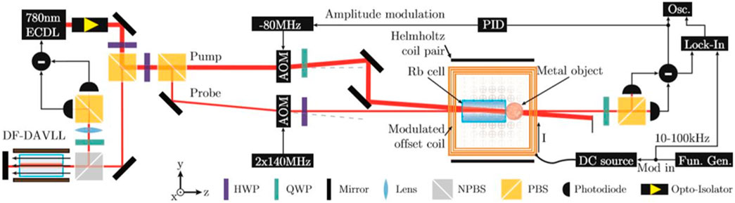
FIGURE 3. Schematic of the atomic magnetometer for magnetic field measurements. Reproduced from Ref. [62], with permission from AIP Publishing.

4.1 Magnetic induction tomography

Identification and imaging of objects are important challenges in many fields. Some equipment such as pipelines and ships will corrode and crack after prolonged use, which may cause serious safety problems. Atomic magnetometers can be used to detect weak magnetic fields for magnetic imaging [63]. The oldest electrical imaging technique is electrical impedance tomography (EIT), which usually involves attaching surface electrodes around the area to be imaged. The technique injects current through the electrodes to the object to be measured and measures the electrical potential, measuring the different distributions of impedance and thus the voltage distribution, which leads to image reconstruction [64].

Magnetic Induction Tomography (MIT) is an important branch of EIT and is an imaging technique based on the principle of electromagnetic imaging [65]. The principle is that under the action of an applied alternating current (AC) excitation magnetic field, the target conductor generates eddy currents due to magnetic induction, and when the target conductor changes, the intensity and distribution of the eddy currents will also change accordingly. The process of imaging using the MIT technique requires the solution of two steps: the first step refers to solving for the spatial distribution of the magnetic field and the output signal of the detection coil when the distributions of the conductivity $\mathrm{\sigma }$ and the magnetic permeabilities $\mathrm{\mu }$ are known. The first step can be viewed as an eddy current problem. Therefore, the complex phasor notation can be used to describe the process in terms of the magnetic vector potential $\overrightarrow{\mathrm{A}}$ under sinusoidal waveform excitation. The spatial distribution of the magnetic field can be obtained by finding the magnetic vector potential [66]:

$\begin{array}{c}\nabla \times \left(\frac{1}{\mathrm{\mu }}\nabla \times \overrightarrow{\mathrm{A}}\right)+\mathrm{i}\mathrm{\omega }\mathrm{\sigma }\overrightarrow{\mathrm{A}}=\overrightarrow{{\mathrm{J}}_{\mathrm{s}}}\end{array}(20)$

Where $\overrightarrow{\mathrm{A}}$ is the magnetic vector potential, $\mathrm{\sigma }$ is the electrical conductivity of the medium, $\mathrm{\mu }$ is the magnetic permeability of the medium, $\mathrm{\omega }$ is angular frequency, and $\overrightarrow{{\mathrm{J}}_{\mathrm{s}}}$ is the current density applied in the excitation coil. When the total current in the excitation coil is ${\mathrm{I}}_0$, the sensitivity of the induced voltage to the conductivity is:

$\begin{array}{c}\frac{\partial {\mathrm{V}}_{\mathrm{m}\mathrm{n}}}{\partial {\mathrm{\sigma }}_{\mathrm{k}}}=-{\mathrm{\omega }}^2\frac{{\int }_{{\mathrm{\Omega }}_{\mathrm{D}\mathrm{k}}}^{\infty }{\mathrm{A}}_{\mathrm{m}}\bullet {\mathrm{A}}_{\mathrm{n}}\mathrm{d}\mathrm{\nu }}{{\mathrm{I}}_0}\end{array}(21)$

Where ${\mathrm{V}}_{\mathrm{m}\mathrm{n}}$ is the measurement voltage, ${\mathrm{\sigma }}_{\mathrm{k}}$ is the conductivity of the pixel $\mathrm{k}$. Pixel $\mathrm{k}$ refers to the volume of the perturbation, which is represented as ${\mathrm{\Omega }}_{\mathrm{D}\mathrm{k}}$. A-m (A-n) is the solution of the forward solver when the excitation (the induction) coil is excited by the current I-0 (the unity current).

The second step is image reconstruction. Researchers often use algorithms to find the distribution of the electrical and magnetic permeability in the field space of the object to be measured, given the known characteristics of the excitation field (e.g., operating frequency, magnetic induction strength in a null field, equations of the magnetic field space, etc.), the detection signal and the boundary conditions of the sensor. The linear method based on Tikhonov regularization [67] is generally considered in image reconstruction, which can be implemented by means of matrix operations:

$\begin{array}{c}\overrightarrow{\mathrm{x}}={\left({\mathbf{J}}^{\mathrm{T}}\mathbf{J}+\mathrm{\alpha }\mathbf{I}\right)}^{-1}{\mathbf{J}}^{\mathrm{T}}\overrightarrow{\mathrm{z}}\end{array}(22)$

Where $\overrightarrow{\mathrm{x}}$ is the pixel vector, $\overrightarrow{\mathrm{z}}$ is the measurement vector, $\mathbf{J}$ is the Jacobian matrix, $\mathbf{I}$ is the identity matrix, and $\mathrm{\alpha }\ge 0$ is a regularization parameter that determines the amount of regularization and serves as a positive constant chosen to control the size of the solution vector [67, 68].

The MIT system was proposed by Griffiths et al as early as 1999 [69]. They successfully built a single-channel acquisition system with an operating frequency of 10 MHz and used a phase-sensitive detector for the measurements. From their results, the scanned saline solution had conductivity ranging from 0.001 to 6 S/m, covering the range of biological tissues. The measured imaginary part of the magnetic disturbance is proportional to the conductivity of the brine, consistent with the theoretical prediction, and the proportionality constant per S/m is −1.2%. In 2004, Scharfetter et al. investigated the advantages of planar gradiometers (PGRAD) for use at MIT [70]. They built a 16-channel MIT system with a bandwidth range of 50 kHz–1.5 MHz, which was excited with an excitation coil for signal reception, and then the amplified signal was fast Fourier transformed to obtain the corresponding information. The results show that very similar sensitivity maps are obtained for the two different PGRADs which is zero on the coil axis. Most MIT setups rely on a standard coil of wire, or an array of coils, which leads to limitations in sensitivity and bandwidth. To overcome these disadvantages, a proof of concept was realized with a self-oscillating Optical Atomic Magnetometer (OAM). In 2014, Wickenbrock et al. demonstrated magnetic induction tomography (MIT) with an all-optical atomic magnetometer [71]. Three different shaped objects were imaged by the researchers; A 37 × 37 mm square, a 37 mm diameter disk, and an isosceles triangle (37 mm on one side, 30 mm on both sides). All objects were made from 2 mm thick aluminium sheets. The shape and size of the imaging sample are shown in Figure 4. The first row shows the position resolved normalized amplitude of the ac magnetic field signal as detected by the lock-in amplifier. The second row shows the corresponding normalized phase data. The system they built was able to map the electrical conductivity of a conducting object. However, the relative complexity of the instrument, its low-applicability scalability, and its reduced flexibility in terms of operating frequency make the instrument less suitable for practical applications.

FIGURE 4

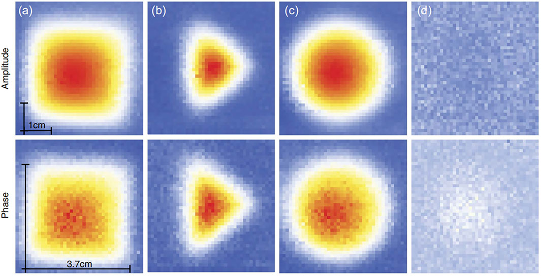
FIGURE 4. Normalized magnetic induction tomography: (A) data for a 37 mm × 37 mm square; (B) isosceles triangle with one side of 37 mm and two sides of 30 mm; (C) disk with 37 mm diameter; (D) an example of the acquisition error,multiplied by a factor of 3 (phase) and 20 (amplitude), to be visible with the respective color coding. Reproduced from Ref. [71], with permission from Optica Publishing Group.

In 2015, Darrer et al. investigated the limitations of electromagnetic imaging through metal enclosures, considering the imaging performance of enclosures of different thicknesses [72]. The experimental results are shown in Figure 5, and the system can image a copper disk when the disk was put in a 20 mm thick aluminum box. The results showed the potential for imaging through shells of other materials such as lead, copper, and iron.

FIGURE 5

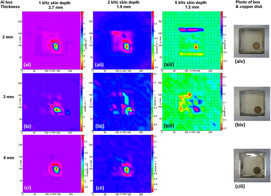
FIGURE 5. Magnetic image capture of a copper disk concealed inside three separate aluminum (Al) box enclosures of thicknesses, 2 mm–5 mm. Reproduced from Ref. [72], with permission from AIP Publishing.

However, to address the sensitivity and bandwidth limitations of a conventional MIT, the researchers looked at a method based on optically pumped atomic magnetometers. The Deans team conducted a series of studies to investigate this method. In 2016, as shown in Figure 6, Deans et al. proposed an electromagnetic induction imaging system based on the radio-frequency optical pump atomic magnetometer (RF OAM), which can be used for materials inspection [73]; Figure 6A is a schematic diagram of the measuring setup. The fundamental sensing unit was an ⁸⁷Rb vapor. The applied magnetic field pumped the light so that ⁸⁷Rb atoms spin polarized along the z direction. The probe beam passed through the gas vapor and polarization rotation, which is measured by projecting the resulting polarization onto z and y. This system not only provided excellent reconstruction of the conductivity map of the target object, but also detected penetration of submillimeter cracks and conductive barriers. This result combined magnetic induction tomography with the highly sensitive properties of atomic magnetometers, demonstrating the potential of a future generation of imaging instruments. The following year, the team used an atomic magnetometer to achieve imaging of copper and aluminum objects located behind ferromagnetic steel and aluminum shields, and the results were shown in Figure 7; [74]. They analyzed the images and used edge detection algorithms to reproduce the size and location of the target accurately. In 2021, the team used a portable RF atomic magnetometer to scan the target object, which can be seen in Figure 8, enabling electromagnetic induction imaging unshielded [75]. In addition, they used a fluxgate magnetometer with a bandwidth of DC-3kHz to limit the bandwidth of the feedback loop and compensate the ambient low-frequency magnetic noise without affecting the application radio frequency of the driving magnetometer. When imaging, they performed a magnetic resonance fit for each position and used the total signal height (Y) at resonance, which greatly reduced the error in the measurement of resonance amplitude. This configuration can meet the standard requirements of typical applications such as security inspection and medical imaging.

FIGURE 6

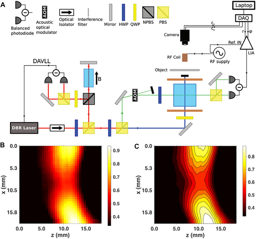
FIGURE 6. (A) Compact RF OAM for MIT; (B,C) Crack detection: high-resolution normalized conductivity map of a sub-mm crack in an Al ring at 10 kHz. Reproduced from Ref. [73], with permission from AIP Publishing.

FIGURE 7

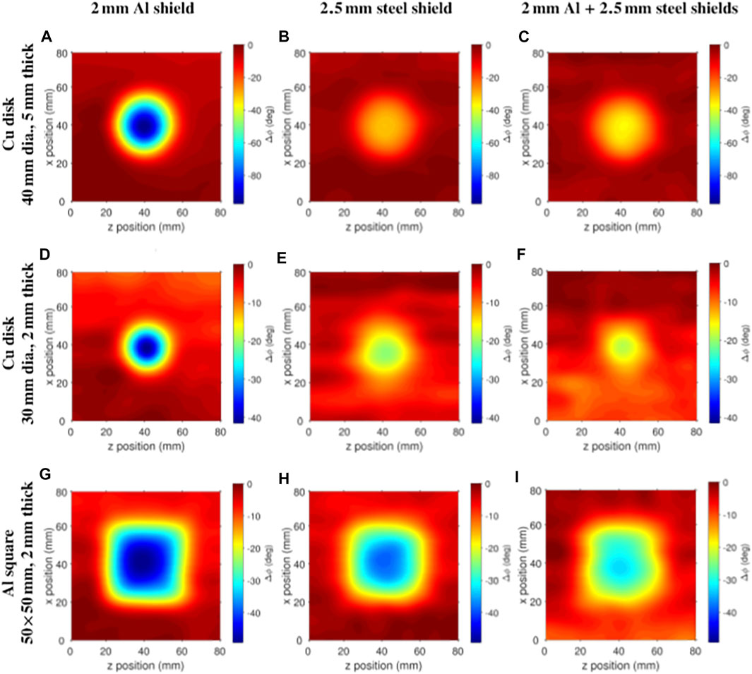
FIGURE 7. Electromagnetic phase imaging through various shields. (A,D,G) 2 mm Al shield; (B,E,H) 2.5 mm ferromagnetic steel shield; (C,F,I) Combination of the 2.5 mm steel shield and 2 mm Al shield. Reproduced from Ref. [74], with permission from Optica Publishing Group.

FIGURE 8

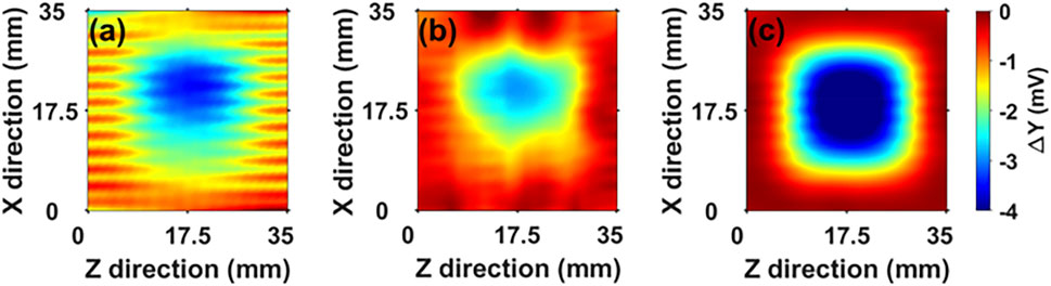
FIGURE 8. Images of conductive objects. (A) The value of Y at 54 kHz. (B) Results obtained with resonance tracking. (C) Results obtained by introducing a detuning of + 800 Hz from the tracked resonance. Reproduced from Ref. [75], with permission from AIP Publishing.

To assess the structural integrity of steelwork and pipelines, Bevington et al. used an atomic magnetometer to enable the imaging of ferromagnetic carbon steel samples and detected thinning of the sample profile in 2018 [76]. The system operates at a relatively high frequency of 12 kHz, and the thickness of carbon steel samples can be detected with a resolution of 0.1 mm. This method can be used for non-destructive dynamic monitoring of steel quality, and can be used for welding condition testing, pipeline testing, corrosion condition of materials and so on. In 2019, Borna et al. developed a pulsed optical pump magnetometer (OPM) array for detecting magnetic field maps generated by arbitrary current distributions [77]. The magnetic source imaging (MSI) system designed by the research team has a 24-channel OPM with a data rate of 500S/s, a sensitivity of 0.8 pT/Hz^1/2, and a dynamic range of 72 dB. By comparing the experimental results with the simulation results, the robustness of the system in capturing the magnetic characteristics of the general planar two-dimensional coil structure is proved. Finally, the current density image of planar two-dimensional coils is successfully reconstructed by using the magnetic field map measured by the pulsed OPM system.

Magnetic Induction Tomography based on atomic magnetometers is a non-destructive inspection technique that avoids the material damage associated with conventional inspection methods. More importantly, it is not limited by the number of coils compared to other forms of tomographic imaging which is shown in Figure 9; [78]. Together with the ultra-high sensitivity of atomic magnetometers, this method allows image reconstruction of the target object at high frequencies. In addition, researchers have experimentally demonstrated that MIT, based on atomic magnetometers, can image objects through certain obstacles. This is an effective and fast method for security screening.

FIGURE 9

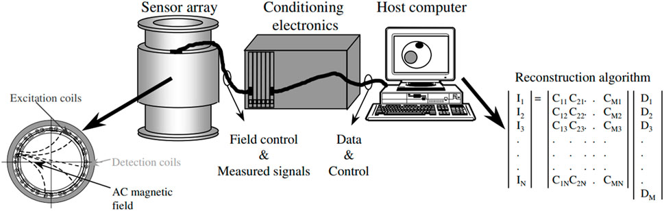
FIGURE 9. The block diagram of a typical MIT system. Reproduced from Ref. [78], with permission from IOP Publishing Ltd.

In the practical application of this method to implement MIT, the target object will often be disturbed by geomagnetic and other environmental noises. Therefore, when designing the measurement system, researchers can use noise compensation to reduce the interference of environmental noise to measurement results. In addition, in the process of image reconstruction, the limited measuring points are discrete and cannot accurately reflect the information of the target image. Therefore, researchers need to use certain image processing algorithms to produce clear images such as fitting measurements.

4.2 Battery testing

With the advantages of high energy density, high output power, no memory effect, and fast charging and discharging rates, lithium-ion batteries have become one of the most used rechargeable electrochemical energy storage devices and are widely used in electronic products, electric vehicles, and grid energy storage systems [79, 80]. However, the practice has seen that lithium batteries still suffer from some unfavorable problems such as the deposition and uncontrolled growth of lithium dendrites and the instability of the solid electrolyte interface layer (SEI) [81, 82]. As the dendrites continue to grow, they are likely to penetrate the diaphragm. Once the diaphragm is penetrated, there is direct contact between the anode and cathode, which usually leads to a short circuit inside the battery, resulting in a thermal runaway or even an explosion of the entire battery. The current distribution within the cell is influenced by the design and resistance distribution of each part of the cell, the heterogeneity of the electrodes, and physical defects such as internal dendrites or cracks and their location. Uneven current distribution is one source of cell failure or capacity loss, and this inhomogeneity is usually caused by lithium dendrite growth or assembly defects. The high energy density of these batteries has led to increasing safety concerns, such as spontaneous combustion and fire accidents in electric vehicles [83–85]. The successive occurrence of such accidents has brought the reliability of batteries into focus.

Non-destructive testing (NDT) on battery condition has received increasing attention for the safety of batteries. Essentially, it refers to a method for identifying discontinuous defects in the material to be tested without causing structural damage. Currently, the commonly used nondestructive testing techniques that can provide in-situ information include X-ray diffraction [86–88], neutron diffraction [89–91], and Raman spectroscopy [92–94]. But these methods can have negative effects like slow speed, alter the properties of the material to be tested, or cause a certain amount of radiation [95]. We can detect magnetic objects using variations in their magnetic field caused by variations in their magnetic susceptibility which is related to the cathode material of the cell [96]. Both positive and negative electrode materials in Li-ion batteries have magnetic materials such as nickel cobalt manganese and graphite. As a result of redox reactions and changes in embedded lithium de-embedding during discharge, the magnetic susceptibility of the electrode material changes, which may result in changes in the induced magnetic field around the battery. According to the Biot-Savart law, changes in currents in a battery will lead to changes in the external magnetic field. Therefore, by measuring changes in the external magnetic field and establishing a relationship between internal defects and abnormal magnetic field images, the condition of the battery can be assessed, and the location of the fault can be determined. A typical battery nondestructive testing experiment setup based on the atomic magnetometer is shown in Figure 10. The magnetic field sensors are placed in this region of negligible field. The battery is placed on a conveyor belt inside a shielded cylinder and is moved by the belt to obtain magnetic field information in the x and z directions.

FIGURE 10

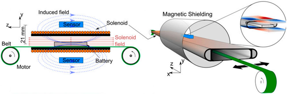
FIGURE 10. Experimental susceptometry setup. Adapted from Ref. [97], with permission from PNAS.

The magnetic field produced by an electric current can be described by the Biot-Savart law [98].

$\begin{array}{c}\overrightarrow{\mathrm{H}}\left(\overrightarrow{\mathrm{r}}\right)=\frac{1}{4\mathrm{\pi }}\int \frac{\mathrm{I}\mathrm{d}\overrightarrow{\mathcal{l}}\times \overrightarrow{{\mathrm{r}}^{\prime }}}{{\left|{\mathrm{r}}^{\prime }\right|}^3}\end{array}(23)$

Where $\overrightarrow{{\mathrm{r}}^{\prime }}$ is the position vector, $\overrightarrow{\mathrm{H}}\left(\overrightarrow{\mathrm{r}}\right)$ is the magnetic field at the displacement $\overrightarrow{\mathrm{r}}$, $\mathrm{I}$ is the source current, $\mathrm{d}\overrightarrow{\mathcal{l}}$ is the tiny wire element of source current. When the ratio of $\left|\mathrm{d}\mathcal{l}\right|$ to $\left|{\mathrm{r}}^{\prime }\right|$ is small enough (less than 0.1), the Biot-Savart law can be represented as [99]:

$\begin{array}{c}\overrightarrow{\mathrm{H}}\left(\overrightarrow{\mathrm{r}}\right)=\frac{1}{4\mathrm{\pi }}{\displaystyle \sum _{\mathrm{k}=1}^{\mathrm{N}}}\frac{{\mathrm{I}}_{\mathrm{k}}\mathrm{d}\overrightarrow{{\mathcal{l}}_{\mathrm{k}}}\times \overrightarrow{{\mathrm{r}}_{\mathrm{k}}^{\prime }}}{{\left|{\mathrm{r}}_{\mathrm{k}}^{\prime }\right|}^3}\end{array}(24)$

$\mathrm{N}$ indicates the number of current elements.

In the field of battery testing, we often need external information such as magnetic fields to assess the health of the battery or to locate defects in the battery, in addition to assessing the effect of magnetic fields generated by the battery on the human body. However, we are often unable to diagnose the state of the battery during operation [100], unable to identify the marker factors that affect the battery life, or the device is too large to be detected [101]. In 2020, scientists from Johannes-Gutenberg University (JGU) and the Helmholtz Institute Mainz (HIM) in Germany proposed a non-contact method for detecting the state of charge of lithium-ion batteries and defects [97]. As shown in Figure 10, They used an atomic magnetometer to measure the weakly induced magnetic field around lithium-ion batteries in a magnetically shielded environment and used the measurement data of the magnetometer to describe the magnetic susceptibility of the battery, reflecting the relationship between the state of local charge and the Internal defect of the battery. The magnetometers can achieve a sensitivity of 20 fT/Hz^1/2. In such an arrangement the current sensitivity could approach 8 nA. The method provides an effective and rapid tool for battery diagnosis and can be implemented in a cost-effective and scalable manner. This measurement capability is of great significance to battery academic research and industry.

To compare the effectiveness of different types of magnetometers for measuring operational and defective commercial batteries, in the same year, Yinan et al. used commercial SQUIDs and atomic magnetometers to test lithium-ion rechargeable batteries (LIBs), as shown in Figure 11; [102]. Their results show that the atomic magnetometer has sufficient sensitivity to characterize defects in the cell. This non-contact, rapid diagnostic method could become a powerful tool for analyzing the condition of different batteries.

FIGURE 11

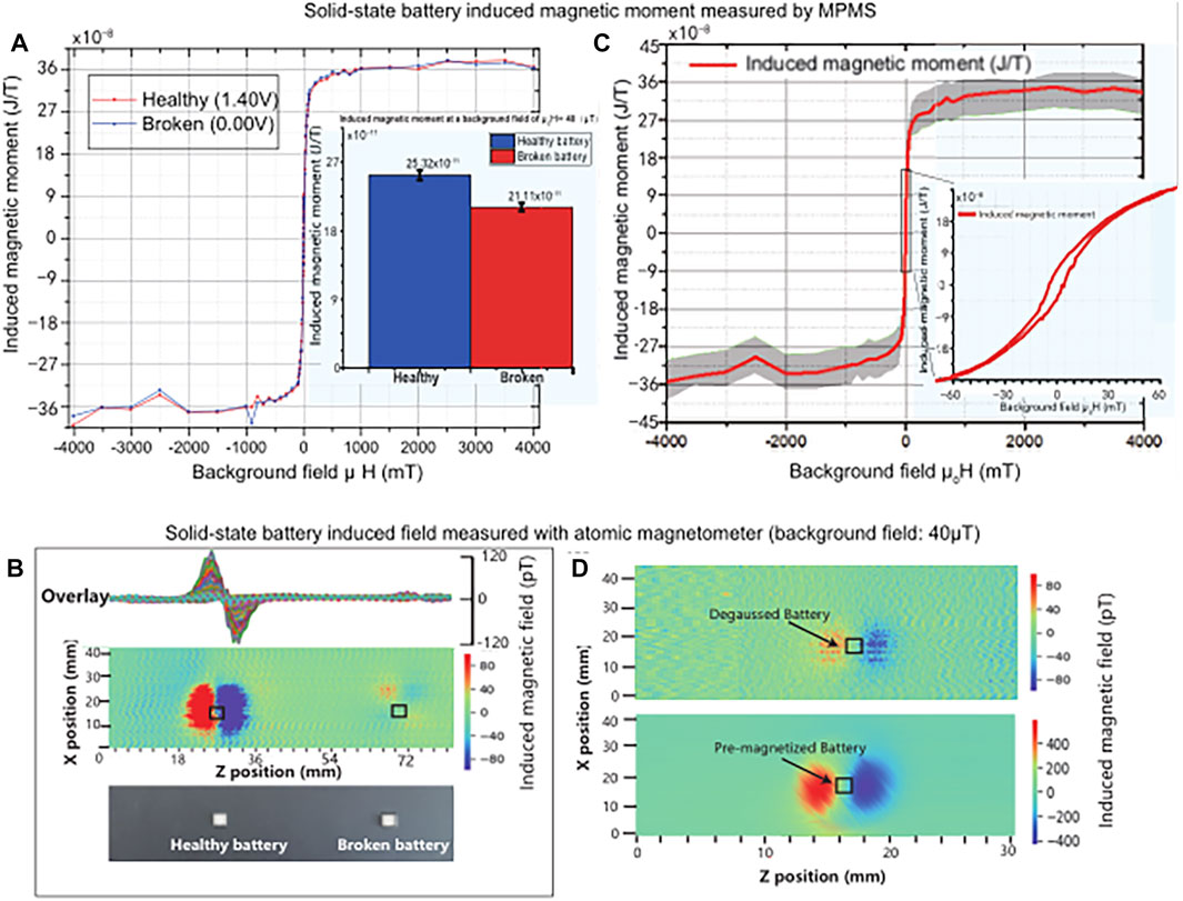
FIGURE 11. (A,C) Induced magnetic moment measurements using SQUID-based MPMS. (B,D) Induced magnetic field maps using the atomic magnetometer setup. Reproduced from Ref. [102], with permission from MDPI.

In 2022, Wang et al. proposed an in-situ detection technology for the capacity consistency of power battery packs based on magnetic field scanning imaging, as shown in Figure 12 [103]. Figure 12A shows the experimental setup for magnetic field scanning. During measurement, the magnetic field components ${\mathrm{B}}_{\mathrm{x}}$, ${\mathrm{B}}_{\mathrm{y}}$ and ${\mathrm{B}}_{\mathrm{z}}$ around the battery can be measured by moving a fluxgate on the battery surface. Figure 12B shows what happens when problem cells are located at different locations in two parallel battery packs. The distribution of the magnetic field is related to the location of the abnormal battery; Figure 12C shows the principal component analysis (PCA) of Figure 12B. The different PCA scores divide the different locations of the problem battery into four quadrants. The distribution characteristics of abnormal cells 1 and 3 are between cell 1 and cell 3, and the same is true for abnormal cells 2 and 4, which means magnetic field distribution characteristics are closely related to the location of the abnormal cell. This technology enables in-situ non-destructive testing of cell-level capacity consistency within the battery pack. The technology can not only assess the consistency of battery capacity but also determine the location of battery failure. It has great application potential in material testing, especially in the field of battery material testing.

FIGURE 12

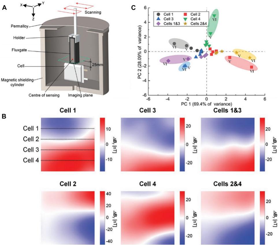
FIGURE 12. (A) Experimental setup and magnetic field measurement of a single cell. (B) Magnetic field maps with the cell having the lower capacity (marked at top of the maps) at different positions; the maps are acquired when discharging 4,250 mAh. (C) PCA results of magnetic field maps at six locations. Reproduced from Ref. [103], with permission from John Wiley and Sons.

As a battery test method that has been studied and applied in recent years, magnetic field measurement uses magnetic field sensors to directly measure the induced magnetic field outside the battery, and then evaluates the battery state by analyzing the induced magnetic field changes. As sensors with high sensitivity, atomic magnetometers can reproduce the nT-level magnetic field around working batteries. By analyzing the magnetic field information, we can then obtain changes in the material inside the batteries, which can reveal more about the charging state of the batteries, or simply realize the classification of healthy and faulty batteries.

At present, the battery detection method based on precision magnetic field measurement has just emerged, so the correlation mechanism theory of induced magnetic field and battery internal factors is not perfect. Researchers can combine theoretical simulations with experimental measurements to explore the relationship between these factors and develop a more mature system of test methods. In addition, in practical applications, lithium batteries are often organized into battery packs. Therefore, how to locate battery pack faults will become a major research direction.

4.3 Underwater target detection and tracking

Conventional optical or acoustic methods often fail to achieve the desired results when detecting underwater targets with great accuracy. Optical methods are affected by water opacity and turbulence [104], while acoustic methods are disturbed by echoes [105, 106], and weak magnetic detection techniques can effectively prevent these interference factors. At the beginning of this century, with the rapid development of electronic measurement technology, computer technology and deep-sea technology, the sensitivity and stability of ocean scalar magnetometer represented by atomic magnetometer and ocean vector magnetometer represented by fluxgate magnetometer are constantly improving. The continuous improvement of magnetic field sensors makes magnetic exploration not only applicable to the fields of marine geology and geophysics, but also to underwater military anti-submarine, submarine pipeline detection, marine geomagnetic navigation, and other applications.

When using a magnetometer to detect underwater magnetic targets, to ensure a better detection effect, it is necessary to reasonably select the detection distance and the detection height of the magnetometer. In underwater detection, the analysis of magnetic anomalous modulus is very important. In 2000, Stavrev and Gerovska proposed four kinds of magnetic anomaly amplitude transform parameters (magnitude magnetic transforms, MMTs), and at the same time systematically analyzed the characteristics of magnetic anomaly moduli [107].

After the 1950s, the detection technology of underwater magnetic targets developed rapidly. In 2002, Gee and Cande developed a three-component magnetometer system that contains a vector magnetometer inside, which can complete data measurement under the drag of normal survey speed [108]. The results of the tests, compared with earlier vector aeromagnetic measurements, showed that the towed instrument can resolve horizontal and vertical anomalies with amplitudes of >30–50 nT. The instrument is particularly useful in equatorial regions where the vector anomalies are much larger than the corresponding full-field anomalies. In 2008, Tian used a dual-frequency side-scan sonar, a high-resolution sub-bottom profiler, and a magnetometer to survey five underwater pipelines which had different outer diameters off the southwestern coast of Taiwan [109]. The water depth range of the measurement area was 10 m–17 m. The depth of buried pipes detected ranged from 0.5 to 3 m. The remaining four profiles showed pipe heights ranging from 0.2 m to 1.2 m. The results show that the continuous wave pulsed subsea profiler Klein 532S-101 used in the study is capable of detecting buried pipes greater than 1.0 m in diameter and greater than 3 m in depth. For pipes less than 0.2 m in diameter, the device was unable to provide valid information for their detection. For pipes between 0.2 m and 1.0 m in diameter, further investigation is required to reach a comprehensive conclusion. The magnetometer can provide qualitative information on the presence of metallic pipes at the time of detection; in shallow water areas it can be used to identify the presence of buried pipes with outside diameters as small as 0.2 m. This study confirms the need for a multi-sensor approach to complement the evaluation of underwater pipeline projects. In 2016, Liu et al. proposed a new compensation method using a differential magnetic field which can improve the measurement accuracy of geomagnetic measurement systems when exploring underwater magnetic objects [110]. With the continuous development of atomic magnetometer technology, it has moved towards practical use, which will drive the overall jump in the level of weak magnetic detection.

To facilitate accurate measurement, detection, and location of magnetic targets submerged underwater, an array of atomic magnetometers may be formed. In 2018, as shown in Figure 13, Deans et al. presented a proof-of-concept demonstration of underwater target detection and localization using atomic magnetometer arrays (AMs) in a magnetic induction tomography (MIT) configuration [111]. In their experimental setup shown in Figure 13A, the atomic magnetometer array consisted of four magnetometers S1-S4 in a 2 × 2 planar configuration. An alternating magnetic field perpendicular to the plane of the sensor array was applied, and the target object would induce eddy currents under the action of the external magnetic field. The resulting magnetic signals were collected via a data acquisition board (DAQ) and analyzed in real time via LabVIEW. Figure 13B shows the coordinate grid parallel to the sensor array plane. During measurement, the target object was placed at different coordinate positions to measure the signal response. Figure 13C shows the measured signal strength of the target object which was an aluminum plate. According to the size of the signal response of the four sensors, the specific coordinate position of the target object could be detected. This technique can be used to extend the magnetometer array to practical applications. In addition, this technique can be used in any body of water and is not restricted by geography.

FIGURE 13

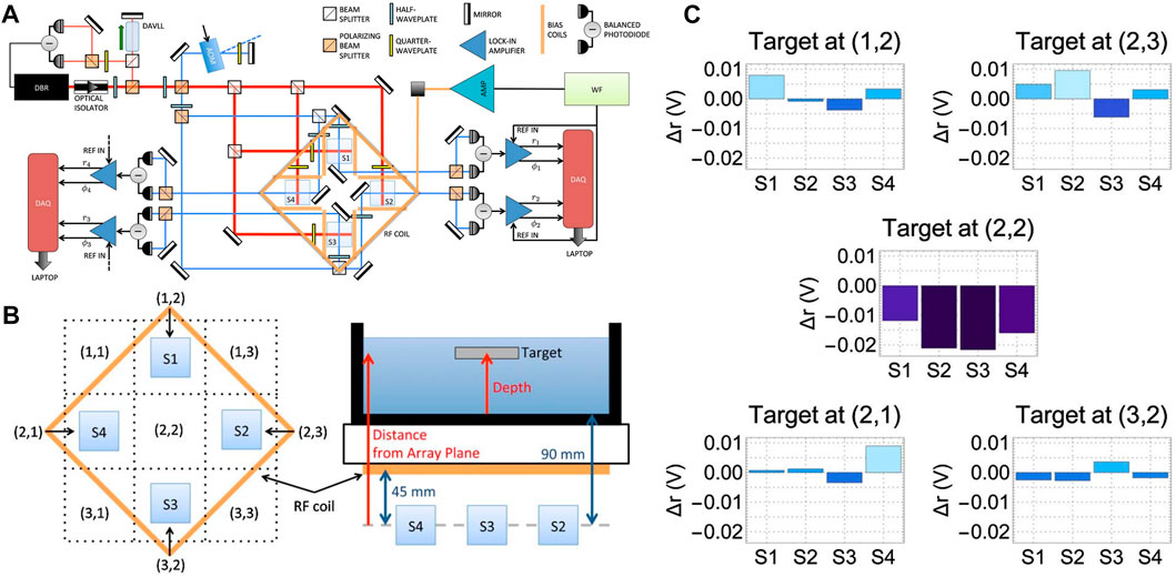
FIGURE 13. (A) Simplified sketch of the 2 × 2 RF AMs array for detection and localization. DBR: distributed Bragg reflector laser. DAVLL: dichroic atomic vapor laser lock; AOM: acousto-optic modulator; DAQ: data acquisition board; AMP: current amplifier; WF: waveform generator; REF IN,reference input; ${\mathrm{r}}_{\mathrm{n}}$ and ${\mathrm{\varphi }}_{\mathrm{n}}$, respectively, are the amplitude and phase signals of the nth sensor Sn; (B) The arrangement for detection and localization; (C) Underwater target detection and localization: simultaneously recorded Δr, when an Al plate (105 mm × 110 mm × 10 mm) is placed in different positions, at 30 mm underwater (120 mm from the array plane). Operation frequency: 10 kHz. Reproduced from Ref. [111], with permission from Optica Publishing Group.

To monitor and detect underwater targets in real-time, atomic magnetometers or atomic magnetometers arrays have been integrated into autonomous underwater vehicles (AUVs). The representative one is the system proposed by Allen et al. in 1997 [112]. This system can work on the AUV’s computer in real-time and overcome interference from the AUV itself. Using this system, multiple vehicle control theory and operations, coastal oceanographic surveys, microscale turbulence surveys, autonomous docking testing and demonstration, and hydrographic surveys of coastal waters can be realized. In 2020, Gallimore et al. developed a scalar magnetometer payload to integrate into a two-man portable autonomous underwater vehicle (AUV) for geophysical and archeological surveys [113]. They collected data using a Geometrics microfabricated atomic magnetometer and a total-field atomic magnetometer. The system combined onboard target detection and autonomous reacquires capability, increasing the effective survey coverage rate of the AUV-based magnetic sensing system. In future research on underwater detection systems, it can be predicted that people will further focus on multi-target detection and improve the anti-jamming ability of the system, to obtain more accurate signals.

The above studies indicate that the underwater detection method based on atomic magnetometers can detect the target object more accurately and eliminate optical or acoustic interference due to the tunability and high sensitivity of the atomic magnetometer array. Depending on different geographical and water conditions, atomic magnetometers can be integrated into different instruments to greatly improve the effective coverage of the system’s measurements. At present, airborne systems equipped with precision magnetic field sensors have been used for underwater detection, but only for detection. Combined with the MIT model mentioned above, target positioning and imaging can be achieved, providing a more functional solution for underwater measurement and monitoring.

4.4 Magnetic communication

There are challenges such as information security, and electromagnetic interference in modern radio communication [114]. One possible solution to these problems is to use magnetic communication to transmit information. Magnetic communication based on electromagnetic principles has been rapidly developed in recent years because the magnetic permeability is little affected by media such as water and soil [115–117].

In traditional magnetic communication, coils are used to detect the induced magnetic field. Their sensitivity increases with increasing signal frequency. In other words, under the low frequency operation the sensitivity reduces, which is not preferable for detecting low frequency signals. Therefore, other methods are needed to detect weak magnetic fields in the low frequency range [118]. Researchers usually reduce the frequency to improve the transmission distance, which requires the production of a longer antenna, greatly increasing the cost and power consumption of the equipment and limiting the communication security. It is difficult to use this method when large-scale communication nodes are deployed [119]. At the same time, this method is limited by bandwidth and sensitivity.

As a kind of high-sensitivity sensor, an atomic magnetometer has higher field sensitivity than the traditional magnetic communication induction coil and can reach noise floors below 1 fT/Hz^1/2 [29]. To detect smaller, more precise signals, researchers are beginning to explore the possibility of using precision magnetic field sensors such as atomic magnetometers for magnetic communication. Magnetic field information at the receiving end can be obtained by using an atomic magnetometer as the receiver of magnetic communication.

In 2017, Gerginov et al. proposed a single-channel low-data-rate RF communication link based on an optically pumped atomic magnetometer and used binary phase shift keying (BPSK) to modulate the signal in order to solve the low-frequency magnetic field bandwidth reduction caused by the reduction of channel capacity and location accuracy [120]. As shown in Figure 14, this method used an optical pump magnetometer as a sensor, which greatly improved the sensitivity of detection. The magnetometer was set to work in direct current (DC), zero-field (ZF), and self-oscillating (SO) modes. The first two modes were used to detect magnetic field modulation, and the other one was used to monitor the total magnetic field variation. In the DC mode, the pump light was modulated at half of the Larmor precession frequency, and the lock-in amplifier L1 was used to detect the polarization modulation signal after resonance. In the ZF mode, the magnitude of the static magnetic field at the magnetometer’s position was set to zero. The pump laser beam is not modulated, and it creates atomic polarization along its direction (x-axis). The polarimeter detects a zero-field resonance which could be demodulated by lock-in amplifier L2. In the SO mode, the reference for the amplitude modulation is phase-locked to the rectified polarimeter output. Figure 14B represents the case where the ambient noise is 300 fT. Using the method in this paper, researchers could reduce the impact of the ambient noise and extended the measurement range to 320 m. By utilizing the intrinsic sensitivity of the magnetometer below 1 pT/Hz^1/2 and using the 1 kHz operating bandwidth of the BPSK signal, they demonstrated ranging enhancement. In 2019, Hott et al. used a high-sensitivity broadband magnetic field sensor to replace the receiving coil of the traditional magnetic induction communication system [116]. The results show that sensitive magnetic field sensors have decisive advantages, including a higher communication range for small receiving units. This approach supports many mobile applications with limited receiver sizes, possibly in combination with multiple detectors.

FIGURE 14

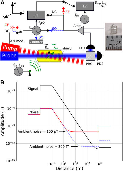
FIGURE 14. (A) Magnetic field sensor setup. The signal routes for the three magnetometer configurations are shown with solid (DC, black), dashed (SO, blue), and dotted (ZF, red) lines. PD: photodetector; PBS: polarizing beam spliter; L: lock-in amplifier; Ampl: amplifier; (B) Link calculation analysis for the magnetic field signal and noise (solid curves) at 1 Hz bandwidth. Reproduced from Ref. [120], with permission from AIP Publishing.

In 2021, Lee et al. used a single-channel rubidium atomic radio frequency magnetometer (RFAM) as a receiver to receive the Zeeman splitting resonance magnetic signal of the ground state of rubidium atoms [121]. They optimized the performance of the RFAM by recording the response signal and signal-to-noise ratio (SNR) at various parameters and obtained a noise level of 159 fT/Hz^1/2 at around 30 kHz. When using a resonant RFAM with a peak amplitude of 8.0 nT, the bandwidth is approximately 650 Hz, and the SNR is approximately 88 dB. The RFAM using alkali atoms is suitable for receiving signals from very low frequency (VLF) carriers in the frequency range from 3 kHz to 30 kHz. This study shows the new capabilities of RFAM in applications based on magnetic signals from low-frequency carriers, which are expected to overcome barriers and expand the communication space with highly magnetically sensitive RFAMs.

In the field of communication, acoustic communication has a narrow band width and a low transmission rate. Compared with acoustic communication, optical communication has a higher transmission rate, but it is prone to absorption and scattering, high equipment costs, easy pollution and damage, and communication distance is seriously affected by the medium. Magnetic field communication under low frequency conditions has the advantages of less influence by medium, stable signal and fast transmission rate. Using atomic magnetometers as the receiver can overcome the shortcomings of long antenna and low bandwidth of traditional magnetic field communication and realize high sensitivity signal detection. In the future, improving SNR and increasing bandwidth will become the main research direction of magnetic communication based on the atomic magnetometer. To achieve this goal, researchers can use signal processing techniques to average out unrelated fluctuations from the environment, eliminating system fluctuations and reducing ambient noise.

5 Conclusion

This paper reviews the principle of weak magnetic detection based on atomic magnetometers, and the application of atomic magnetometers in magnetic imaging, battery testing, underwater target detection and tracking, and magnetic communication. In the field of magnetic imaging, the MIT system based on atomic magnetometers measures the magnetic signal changes caused by eddy current changes in the target object and uses image reconstruction algorithms to reproduce the structure diagram of the target object. To monitor changes in the magnetic field around cells in real time, atomic magnetometers are used as magnetic sensors in battery testing. To reflect the characteristics of materials without contact and damage, including surface, battery testing using this technique is a type of non-destructive testing. In the field of underwater target detection and tracking, the atomic magnetometer can overcome the shortcomings of traditional optical and acoustic methods, overcome the influence of hydrological conditions, and accurately detect underwater magnetic signals. These high-precision magnetic measurement technologies have the ability to detect sinking and underwater collisions of ships, which is of utmost importance in the pursuit and identification of magnetic objects submerged in water. Signal processing can be utilized to achieve accurate and reliable communication of magnetic signals. This is accomplished by using an atomic magnetometer to receive the Zeeman split resonant magnetic signal within the field of magnetic communication. At present, atomic magnetometers are not yet reaching their full potential, and there is still room for improvement in practical miniaturized atomic magnetometer sensitivity compared to large-scale magnetic field measuring devices. In conclusion, the use of atomic magnetometers in related fields has developed into a current research hotspot, and the results of this practical application research continue to encourage continuous optimization of the performance of atomic magnetometers.

Author contributions

XB wrote the initial draft and led the further development of the manuscript. KW, DP, SL, and LL contributed to editing and revising of the manuscript. All authors contributed to the article and approved the submitted version.

Funding

This work was supported by the National Key Research and Development Program (Grant No. 2022YFC2204402), Guangdong Science and Technology Project (Grant No. 20220505020011), Shenzhen Science and Technology Program (Grant No. 2021Szvup172), and Shenzhen Science and Technology Program (Grant No. JCYJ20220818102003006).

Conflict of interest

The authors declare that the research was conducted in the absence of any commercial or financial relationships that could be construed as a potential conflict of interest.

Publisher’s note

All claims expressed in this article are solely those of the authors and do not necessarily represent those of their affiliated organizations, or those of the publisher, the editors and the reviewers. Any product that may be evaluated in this article, or claim that may be made by its manufacturer, is not guaranteed or endorsed by the publisher.

References

1. Minelli L, Speranza F, Nicolosi I, Caracciolo FD, Carluccio R, Chiappini S, et al. Aeromagnetic investigation of the central apennine seismogenic zone (Italy): From basins to faults. Tectonics (2018) 37(5):1435–53. doi:10.1002/2017tc004953

CrossRef Full Text | Google Scholar

2. Ouyang XY, Liu WL, Xiao Z, Hao YQ. Observations of ULF waves on the ground and ionospheric Doppler shifts during storm sudden commencement. J Geophys Res-space Phys (2016) 121(4):2976–83. doi:10.1002/2015ja022092

CrossRef Full Text | Google Scholar

3. Lyskowski M, Pasierb B, Wardas-Lason M, Wojas A. Historical anthropogenic layers identification by geophysical and geochemical methods in the Old Town area of Krakow (Poland). Catena (2018) 163:196–203. doi:10.1016/j.catena.2017.12.012

CrossRef Full Text | Google Scholar

4. Zhao GY, Han Q, Peng X, Zou PY, Wang HD, Du CP, et al. An aeromagnetic compensation method based on a multimodel for mitigating multicollinearity. Sensors (2019) 19(13):13. doi:10.3390/s19132931

PubMed Abstract | CrossRef Full Text | Google Scholar

5. Forrester R, Huq MS, Ahmadi M, Straznicky P. Magnetic signature attenuation of an unmanned aircraft system for aeromagnetic survey. Ieee-asme Trans Mechatron (2014) 19(4):1436–46. doi:10.1109/tmech.2013.2285224

CrossRef Full Text | Google Scholar

6. Adepelumi AA, Fontes SL, Schnegg PA, Flexor JM. An integrated magnetotelluric and aeromagnetic investigation of the Serra da Cangalha impact crater, Brazil. Phys Earth Planet Inter (2005) 150(1-3):159–81. doi:10.1016/j.pepi.2004.08.029

CrossRef Full Text | Google Scholar

7. Hämäläinen M, Hari R, Ilmoniemi RJ, Knuutila J, Lounasmaa OV. Magnetoencephalography---theory, instrumentation, and applications to noninvasive studies of the working human brain. Rev Mod Phys (1993) 65(2):413–97. doi:10.1103/RevModPhys.65.413

CrossRef Full Text | Google Scholar

8. Boto E, Holmes N, Leggett J, Roberts G, Shah V, Meyer SS, et al. Moving magnetoencephalography towards real-world applications with a wearable system. Nature (2018) 555(7698):657. doi:10.1038/nature26147

PubMed Abstract | CrossRef Full Text | Google Scholar

9. George MS, Lisanby SH, Sackeim HA. Transcranial magnetic stimulation - applications in neuropsychiatry. Arch Gen Psychiatry (1999) 56(4):300–11. doi:10.1001/archpsyc.56.4.300

PubMed Abstract | CrossRef Full Text | Google Scholar

10. Herrera-May AL, Aguilera-Cortes LA, Garcia-Ramirez PJ, Manjarrez E. Resonant magnetic field sensors based on MEMS technology. Sensors (2009) 9(10):7785–813. doi:10.3390/s91007785

PubMed Abstract | CrossRef Full Text | Google Scholar

11. Froidurot B, Rouve LL, Foggia A, Bongiraud JP, Meunier G. Magnetic discretion of naval propulsion machines. IEEE Trans Magn (2002) 38(2):1185–8. doi:10.1109/20.996303

CrossRef Full Text | Google Scholar

12. Alberto N, Domingues MF, Marques C, Andre P, Antunes P. Optical fiber magnetic field sensors based on magnetic fluid: A review. Sensors (2018) 18(12):27. doi:10.3390/s18124325

CrossRef Full Text | Google Scholar

13. Auster HU, Fornacon KH, Georgescu E, Glassmeier KH, Motschmann U. Calibration of flux-gate magnetometers using relative motion. Meas Sci Tech (2002) 13(7):1124–31. doi:10.1088/0957-0233/13/7/321

CrossRef Full Text | Google Scholar

14. Ripka P. Review of fluxgate sensors. Sensors & Actuators. (1992) 33(3):129–41. doi:10.1016/0924-4247(92)80159-Z

CrossRef Full Text | Google Scholar

15. Ripka P. Magnetic sensors and magnetometers. Meas Sci Tech (2002) 2002. doi:10.1088/0957-0233/13/4/707

CrossRef Full Text | Google Scholar

16. Hayashi T, Itozaki H. SQUID probe microscope with through-hole SQUID. Ieee Trans Appl Superconductivity (2005) 15(2):737–40. doi:10.1109/tasc.2005.850031

CrossRef Full Text | Google Scholar

17. Weinstock H. A review of SQUID magnetometry applied to nondestructive evaluation. IEEE Trans Magn (1991) 27(2):3231–6. doi:10.1109/20.133898

CrossRef Full Text | Google Scholar

18. Vrba J, Betts K, Burbank M. Whole cortex, 64 channel SQUID biomagnetometer system. IEEE Trans Appl Supercond (1993) 3(1):1878–82. doi:10.1109/77.233314

CrossRef Full Text | Google Scholar

19. Gong XR, Chen SD, Zhang S, Guo X. JPM-4 proton precession magnetometer and sensitivity estimation. Sens Mater (2021) 34(1):13–26. doi:10.18494/sam3719

CrossRef Full Text | Google Scholar

20. Shahsavani H. Comparison of a low-cost magneto-inductive magnetometer with a proton magnetometer: A case study on the galali iron ore deposit in Western Iran. Near Surf Geophys (2019) 17(1):69–84. doi:10.1002/nsg.12026

CrossRef Full Text | Google Scholar

21. Denisov AY, Denisova OV, Sapunov VA, Khomutov SY. Measurement quality estimation of proton-precession magnetometers. Earth Planets Space (2006) 58(6):707–10. doi:10.1186/bf03351971

CrossRef Full Text | Google Scholar

22. Karsenty A. A comprehensive review of integrated Hall effects in macro-, micro-, nanoscales, and quantum devices. Sensors (2020) 20(15):32. doi:10.3390/s20154163

PubMed Abstract | CrossRef Full Text | Google Scholar

23. Popovic RS, Randjelovic Z, Manic D. Integrated Hall-effect magnetic sensors. Sens Actuator A-Phys. (2001) 91(1-2):46–50. doi:10.1016/s0924-4247(01)00478-2

CrossRef Full Text | Google Scholar

24. Jankowski J, El-Ahmar S, Oszwaldowski M. Hall sensors for extreme temperatures. Sensors (2011) 11(1):876–85. doi:10.3390/s110100876

PubMed Abstract | CrossRef Full Text | Google Scholar

25. Li XY, Chen WP, Yin L, Fu Q, Liu XW. A closed-loop Sigma-Delta modulator for a tunneling magneto-resistance sensor. IEICE Electron Express (2017) 14(15):6. doi:10.1587/elex.14.20170700

CrossRef Full Text | Google Scholar

26. Li XY, Hu JP, Liu XW. Study of a closed-loop high-precision front-end circuit for tunneling magneto-resistance sensors. Mod Phys Lett B (2019) 33(8):9. doi:10.1142/s0217984919500854

CrossRef Full Text | Google Scholar

27. Gao L, Chen F, Yao YF, Xu DC. High-precision acceleration measurement system based on Tunnel magneto-resistance effect. Sensors (2020) 20(4):17. doi:10.3390/s20041117

PubMed Abstract | CrossRef Full Text | Google Scholar

28. Kitching J, Knappe S, Donley EA. Atomic sensors - a review. IEEE Sens J (2011) 11(9):1749–58. doi:10.1109/jsen.2011.2157679

CrossRef Full Text | Google Scholar

29. Budker D, Romalis M. Optical magnetometry. Nat Phys (2007) 3(4):227–34. doi:10.1038/nphys566

CrossRef Full Text | Google Scholar

30. Dang HB, Maloof AC, Romalis MV. Ultra-high sensitivity magnetic field and magnetization measurements with an atomic magnetometer. Appl Phys Lett (2010) 97(15):227. doi:10.1063/1.3491215

CrossRef Full Text | Google Scholar

31. Auster HU, Glassmeier KH, Magnes W, Aydogar O, Baumjohann W, Constantinescu D, et al. The THEMIS fluxgate magnetometer. Space Sci Rev (2008) 141(1-4):235–64. doi:10.1007/s11214-008-9365-9

CrossRef Full Text | Google Scholar

32. Carelli P, Castellano MG. High-sensitivity DC-SQUID measurements. Physica B (2000) 280(1-4):537–9. doi:10.1016/s0921-4526(99)01855-4

CrossRef Full Text | Google Scholar

33. Liu H, Dong H, Liu Z, Ge J, Bai B, Zhang C. Noise characterization for the FID signal from proton precession magnetometer. J Instrum (2017) 12:15. doi:10.1088/1748-0221/12/07/p07019

CrossRef Full Text | Google Scholar

34. Ripka P, Janosek M. Advances in magnetic field sensors. IEEE Sens J (2010) 10(6):1108–16. doi:10.1109/jsen.2010.2043429

CrossRef Full Text | Google Scholar

35. Jin ZH, Sam M, Oogane M, Ando Y. Serial MTJ-based TMR sensors in bridge configuration for detection of fractured steel bar in magnetic flux leakage testing. Sensors (2021) 21(2):10. doi:10.3390/s21020668

CrossRef Full Text | Google Scholar

36. Shah VK, Wakai RT. A compact, high performance atomic magnetometer for biomedical applications. Phys Med Biol (2013) 58(22):8153–61. doi:10.1088/0031-9155/58/22/8153

PubMed Abstract | CrossRef Full Text | Google Scholar

37. Scully MO, Fleischhauer M. High-sensitivity magnetometer based on index-enhanced media. Phys Rev Lett (1992) 69(9):1360–3. doi:10.1103/PhysRevLett.69.1360

PubMed Abstract | CrossRef Full Text | Google Scholar

38. Nagel A, Graf L, Naumov A, Mariotti E, Biancalana V, Meschede D, et al. Experimental realization of coherent dark-state magnetometers. Europhysics Lett (1998) 44(1):31. doi:10.1209/epl/i1998-00430-0

CrossRef Full Text | Google Scholar

39. Budker D, Kimball DF, Rochester SM, Yashchuk VV. Nonlinear magneto-optical rotation via alignment-to-orientation conversion. Phys Rev Lett (2000) 85(10):2088–91. doi:10.1103/PhysRevLett.85.2088

PubMed Abstract | CrossRef Full Text | Google Scholar

40. Kimball DFJ, Jacome LR, Guttikonda S, Bahr EJ, Chan LF. Magnetometric sensitivity optimization for nonlinear optical rotation with frequency-modulated light: Rubidium D2 line. J Appl Phys (2009) 106(6):15. doi:10.1063/1.3225917

CrossRef Full Text | Google Scholar

41. Allred JC, Lyman RN, Kornack TW, Romalis MV. High-sensitivity atomic magnetometer unaffected by spin-exchange relaxation. Phys Rev Lett (2002) 89(13):4. doi:10.1103/PhysRevLett.89.130801

PubMed Abstract | CrossRef Full Text | Google Scholar

42. Kominis IK, Kornack TW, Allred JC, Romalis MV. A subfemtotesla multichannel atomic magnetometer. Nature (2003) 422(6932):596–9. doi:10.1038/nature01484

PubMed Abstract | CrossRef Full Text | Google Scholar

43. Murzin D, Mapps DJ, Levada K, Belyaev V, Omelyanchik A, Panina L, et al. Ultrasensitive magnetic field sensors for biomedical applications. Sensors (2020) 20(6):32. doi:10.3390/s20061569

PubMed Abstract | CrossRef Full Text | Google Scholar

44. Bennett JS, Vyhnalek BE, Greenall H, Bridge EM, Gotardo F, Forstner S, et al. Precision magnetometers for aerospace applications: A review. Sensors (2021) 21(16):27. doi:10.3390/s21165568

CrossRef Full Text | Google Scholar

45. Liu XJ, Bi WH, Li Y, Hu YH, Chang M, Zhang XD. A review of fiber-coupled atomic magnetometer. Microwave Opt Tech Lett (2022) 2022. doi:10.1002/mop.33497

CrossRef Full Text | Google Scholar

46. Aslam N, Zhou HY, Urbach EK, Turner MJ, Walsworth RL, Lukin MD, et al. Quantum sensors for biomedical applications. Nat Rev Phys (2023) 13. doi:10.1038/s42254-023-00558-3

CrossRef Full Text | Google Scholar

47. Budker D. Atomic physics - a new spin on magnetometry. Nature (2003) 422(6932):574–5. doi:10.1038/422574a

PubMed Abstract | CrossRef Full Text | Google Scholar

48. Nara T, Suzuki S, Ando S. A closed-form formula for magnetic dipole localization by measurement of its magnetic field and spatial gradients. IEEE Trans Magn (2006) 42(10):3291–3. doi:10.1109/tmag.2006.879151

CrossRef Full Text | Google Scholar

49. Gerovska D, Arauzo-Bravo MJ, Stavrev P. Determination of the parameters of compact ferro-metallic objects with transforms of magnitude magnetic anomalies. J Appl Geophys (2004) 55(3-4):173–86. doi:10.1016/j.jappgeo.2003.10.001

CrossRef Full Text | Google Scholar

50. Primdahl F, Risbo T, Merayo JMG, Brauer P, Toffner-Clasuen L. In-flight spacecraft magnetic field monitoring using scalar/vector gradiometry. Meas Sci Tech (2006) 17(6):1563–9. doi:10.1088/0957-0233/17/6/038

CrossRef Full Text | Google Scholar

51. Bracken RE, Brown PJ. Reducing tensor magnetic gradiometer data for unexploded ordnance detection. First Break (2005) 23(8):63. doi:10.3997/1365-2397.23.8.26662

CrossRef Full Text | Google Scholar

52. Queitsch M, Schiffler M, Stolz R, Rolf C, Meyer M, Kukowski N. Investigation of 3D magnetisation of a dolerite intrusion using airborne full tensor magnetic gradiometry (FTMG) data. Geophys J Int (2019) 3:3. doi:10.1093/gji/ggz104

CrossRef Full Text | Google Scholar

53. Otnes R. Oceans 2007 - europe - static magnetic dipole detection using vector linear prediction, Anderson functions, and block-based adaptive processing In: Ieee oceans 2007. Scotland, UK: Europe - Aberdeen (2007). p. 1–6. doi:10.1109/oceanse.2007.4302288

CrossRef Full Text | Google Scholar

54. Hu C, Meng MQH, Mandal M. A linear algorithm for tracing magnet position and orientation by using three-axis magnetic sensors. IEEE Trans Magn (2007) 43(12):4096–101. doi:10.1109/tmag.2007.907581

CrossRef Full Text | Google Scholar

55. Pedersen LB, Rasmussen TM. The gradient tensor of potential field anomalies: Some implications on data collection and data processing of maps. Geophysics (1990) 55(12):1558–66. doi:10.1190/1.1442807

CrossRef Full Text | Google Scholar

56. Wynn WM, Frahm CP, Carroll PJ, Clark RH, Wynn MJ. Advanced superconducting gradiometer/Magnetometer arrays and a novel signal processing technique. Magnetics IEEE Trans (1975) 11(2):701–7. doi:10.1109/TMAG.1975.1058672

CrossRef Full Text | Google Scholar

57. Luo Y, Wu MP, Wang P, Duan SL, Liu HJ, Wang JL, et al. Full magnetic gradient tensor from triaxial aeromagnetic gradient measurements: Calculation and application. Appl Geophys (2015) 12(3):283–91. doi:10.1007/s11770-015-0508-y

CrossRef Full Text | Google Scholar

58. Wang YF, Rong LL, Qiu LQ, Lukyanenko DV, Yagola AG. Magnetic susceptibility inversion method with full tensor gradient data using low-temperature SQUIDs. Pet Sci (2019) 16(4):794–807. doi:10.1007/s12182-019-0350-6

CrossRef Full Text | Google Scholar

59. Borna A, Carter TR, Goldberg JD, Colombo AP, Jau YY, Berry C, et al. A 20-channel magnetoencephalography system based on optically pumped magnetometers. Phys Med Biol (2017) 62(23):8909–23. doi:10.1088/1361-6560/aa93d1

PubMed Abstract | CrossRef Full Text | Google Scholar

60. Liu Z, Zou S, Yin KF, Zhou BQ, Ning XL, Yuan H. Lifetime estimation model of vapor cells in atomic magnetometers. J Phys D-appl Phys (2022) 55(28):9. doi:10.1088/1361-6463/ac677b

CrossRef Full Text | Google Scholar

61. Korth H, Kitching JE, Bonnell JW, Bryce BA, Clark GB, Edens WK, et al. Flight demonstration of a miniature atomic scalar magnetometer based on a microfabricated rubidium vapor cell. Rev Sci Instrum (2023) 94(3):11. doi:10.1063/5.0135372

CrossRef Full Text | Google Scholar

62. Wickenbrock A, Tricot F, Renzoni F. Magnetic induction measurements using an all-optical Rb-87 atomic magnetometer. Appl Phys Lett (2013) 103(24):4. doi:10.1063/1.4848196

CrossRef Full Text | Google Scholar

63. Griffiths H. Magnetic induction tomography. Meas Sci Tech (2001) 12:1126. doi:10.1088/0957-0233/12/8/319

CrossRef Full Text | Google Scholar

64. Scharfetter H, Riu P, Populo M, Rosell J. Sensitivity maps for low-contrast perturbations within conducting background in magnetic induction tomography. Physiol Meas (2002) 23(1):195–202. doi:10.1088/0967-3334/23/1/320

PubMed Abstract | CrossRef Full Text | Google Scholar

65. Scharfetter H, Kostinger A, Issa S. Hardware for quasi-single-shot multifrequency magnetic induction tomography (MIT): The graz Mk2 system. Physiol Meas (2008) 29(6):S431–S43. doi:10.1088/0967-3334/29/6/s36

PubMed Abstract | CrossRef Full Text | Google Scholar

66. Wei HY, Soleimani M. A magnetic induction tomography system for prospective industrial processing applications. Chin J Chem Eng (2012) 20(2):406–10. doi:10.1016/s1004-9541(12)60404-2

CrossRef Full Text | Google Scholar

67. Calvetti D, Morigi S, Reichel L, Sgallari F. Tikhonov regularization and the L-curve for large discrete ill-posed problems. J Comput Appl Math (2000) 123(1-2):423–46. doi:10.1016/s0377-0427(00)00414-3

CrossRef Full Text | Google Scholar

68. Golub GH, Hansen PC, O'Leary DP. Tikhonov regularization and total least squares. SIAM J Matrix Anal Appl (1999) 21(1):185–94. doi:10.1137/s0895479897326432

CrossRef Full Text | Google Scholar

69. Griffiths H, Stewart WR, Gough W. Magnetic induction tomography - a measuring system for biological tissues. In: PJ Riu, J Rosell, R Bragos, and O Casas editors Electrical bioimpedance methods: Applications to medicine and biotechnology Annals of the New York academy of sciences 873. New York: New York Acad Sciences (1999). p. 335–45.

PubMed Abstract | CrossRef Full Text | Google Scholar

70. Scharfetter H, Rauchenzauner S, Merwa R, Biro O, Hollaus K. Planar gradiometer for magnetic induction tomography (MIT): Theoretical and experimental sensitivity maps for a low-contrast phantom. Physiol Meas (2004) 25(1):325–33. doi:10.1088/0967-3334/25/1/036

PubMed Abstract | CrossRef Full Text | Google Scholar

71. Wickenbrock A, Jurgilas S, Dow A, Marmugi L, Renzoni F. Magnetic induction tomography using an all-optical Rb-87 atomic magnetometer. Opt Lett (2014) 39(22):6367–70. doi:10.1364/ol.39.006367

PubMed Abstract | CrossRef Full Text | Google Scholar

72. Darrer BJ, Watson JC, Bartlett PA, Renzoni F. Electromagnetic imaging through thick metallic enclosures. AIP Adv (2015) 5(8):8. doi:10.1063/1.4928864

CrossRef Full Text | Google Scholar

73. Deans C, Marmugi L, Hussain S, Renzoni F. Electromagnetic induction imaging with a radio-frequency atomic magnetometer. Appl Phys Lett (2016) 108(10):1126. doi:10.1063/5.0056876

CrossRef Full Text | Google Scholar

74. Deans C, Marmugi L, Renzoni F. Through-barrier electromagnetic imaging with an atomic magnetometer. Opt Express (2017) 25(15):17911–7. doi:10.1364/oe.25.017911

PubMed Abstract | CrossRef Full Text | Google Scholar

75. Deans C, Cohen Y, Yao H, Maddox B, Vigilante A, Renzoni F. Electromagnetic induction imaging with a scanning radio frequency atomic magnetometer. Appl Phys Lett (2021) 119(1):5. doi:10.1063/5.0056876

CrossRef Full Text | Google Scholar

76. Bevington P, Gartman R, Chalupczak W, Deans C, Marmugi L, Renzoni F. Non-destructive structural imaging of steelwork with atomic magnetometers. Appl Phys Lett (2018) 113(6):4. doi:10.1063/1.5042033

CrossRef Full Text | Google Scholar

77. Borna A, Carter TR, DeRego P, James CD, Schwindt PDD. Magnetic source imaging using a pulsed optically pumped magnetometer array. IEEE Trans Instrum Meas (2019) 68(2):493–501. doi:10.1109/tim.2018.2851458

PubMed Abstract | CrossRef Full Text | Google Scholar

78. Binns R, Lyons ARA, Peyton AJ, Pritchard WDN. Imaging molten steel flow profiles. Meas Sci Tech (2001) 12(8):1132–8. doi:10.1088/0957-0233/12/8/320

CrossRef Full Text | Google Scholar

79. Liu W, Oh P, Liu X, Lee M, Cho W, Chae S, et al. Nickel-rich layered lithium transition-metal oxide for high-energy lithium-ion batteries. Angew Chem Int Edition (2014) 2014. doi:10.1002/anie.201409262

CrossRef Full Text | Google Scholar

80. Miao Y, Hynan P, Von Jouanne A, Yokochi A. Current Li-ion battery technologies in electric vehicles and opportunities for advancements. Energies (2019) 12(6). doi:10.3390/en12061074

CrossRef Full Text | Google Scholar

81. Wang CX, Odstrcil R, Liu J, Zhong WH. Protein-modified SEI formation and evolution in Li metal batteries. J Energ Chem (2022) 73:248–58. doi:10.1016/j.jechem.2022.06.0172095-4956

CrossRef Full Text | Google Scholar

82. Akai T, Ota H, Namita H, Yamaguchi S, Nomura M. XANES study on solid electrolyte interface of Li ion battery. Physica Scripta (2005) T115:408–11. doi:10.1238/Physica.Topical.115a00408

CrossRef Full Text | Google Scholar

83. Panchal S, Dincer I, Agelin-Chaab M, Fraser R, Fowler M. Transient electrochemical heat transfer modeling and experimental validation of a large sized LiFePO4/graphite battery. Int J Heat Mass Transfer (2017) 109:1239–51. doi:10.1016/j.ijheatmasstransfer.2017.03.005

CrossRef Full Text | Google Scholar

84. Lu L, Han X, Li J, Hua J, Ouyang M. A review on the key issues for lithium-ion battery management in electric vehicles. J Power Sourc (2013) 226(15):272–88. doi:10.1016/j.jpowsour.2012.10.060

CrossRef Full Text | Google Scholar

85. Yao L, Wang Z, Ma J. Fault detection of the connection of lithium-ion power batteries based on entropy for electric vehicles. J Power Sourc (2015) 293(20):548–61. doi:10.1016/j.jpowsour.2015.05.090

CrossRef Full Text | Google Scholar

86. Lim J, Li YY, Alsem DH, So H, Lee SC, Bai P, et al. Origin and hysteresis of lithium compositional spatiodynamics within battery primary particles. Science (2016) 353(6299):566–71. doi:10.1126/science.aaf4914

PubMed Abstract | CrossRef Full Text | Google Scholar

87. Chapman D, Nesch I, Hasnah MO, Morrison TI. X-ray optics for emission line X-ray source diffraction enhanced systems. Nucl Instrum Methods Phys Res Sect A-accel Spectrom Dect Assoc Equip (2006) 562(1):461–7. doi:10.1016/j.nima.2006.02.185

CrossRef Full Text | Google Scholar

88. Muniz FTL, Miranda MAR, dos Santos CM, Sasaki JM. The Scherrer equation and the dynamical theory of X-ray diffraction. Acta Crystallogr Sect A (2016) 72:385–90. doi:10.1107/s205327331600365x

PubMed Abstract | CrossRef Full Text | Google Scholar

89. Fina F, Callear SK, Carins GM, Irvine JTS. Structural investigation of graphitic carbon nitride via XRD and neutron diffraction. Chem Mat (2015) 27(7):2612–8. doi:10.1021/acs.chemmater.5b00411

CrossRef Full Text | Google Scholar

90. Hammond OS, Bowron DT, Edler KJ. Liquid structure of the choline chloride-urea deep eutectic solvent (reline) from neutron diffraction and atomistic modelling. Green Chem (2016) 18(9):2736–44. doi:10.1039/c5gc02914g

CrossRef Full Text | Google Scholar

91. Liu J, Kunz M, Chen K, Tamura N, Richardson TJ. Visualization of charge distribution in a lithium battery electrode. J Phys Chem Lett (2010) 1(14):2120–3. doi:10.1021/jz100634n

CrossRef Full Text | Google Scholar

92. Panitz JC, Novak P, Haas O. Raman microscopy applied to rechargeable lithium-ion cells - steps towards in situ Raman imaging with increased optical efficiency. Appl Spectrosc (2001) 55(9):1131–7. doi:10.1366/0003702011953379

CrossRef Full Text | Google Scholar

93. Frezzotti ML, Tecce F, Casagli A. Raman spectroscopy for fluid inclusion analysis. J Geochem Explor (2012) 112:1–20. doi:10.1016/j.gexplo.2011.09.009

CrossRef Full Text | Google Scholar

94. Talari ACS, Movasaghi Z, Rehman S, Rehman IU. Raman spectroscopy of biological tissues. Appl Spectrosc Rev (2015) 50(1):46–111. doi:10.1080/05704928.2014.923902

CrossRef Full Text | Google Scholar

95. Garcia-Moreno F, Neu TR, Kamm PH, Banhart J. X-Ray tomography and tomoscopy on metals: A review. Adv Eng Mater (2022) 2022(8):28. doi:10.1002/adem.202201355

CrossRef Full Text | Google Scholar

96. Chernova NA, Nolis GM, Omenya FO, Zhou H, Li Z, Whittingham MS. What can we learn about battery materials from their magnetic properties? J Mater Chem (2011) 21(27):9865–75. doi:10.1039/c1jm00024a

CrossRef Full Text | Google Scholar

97. Hu YA, Iwata GZ, Mohammad M, Silletta EV, Wickenbrock A, Blanchard JW, et al. Sensitive magnetometry reveals inhomogeneities in charge storage and weak transient internal currents in Li-ion cells. Proc Natl Acad Sci U S A (2020) 117(20):10667–72. doi:10.1073/pnas.1917172117

PubMed Abstract | CrossRef Full Text | Google Scholar

98. Brauchle F, Grimsmann F, von Kessel O, Birke KP. Direct measurement of current distribution in lithium-ion cells by magnetic field imaging. J Power Sourc (2021) 507:11. doi:10.1016/j.jpowsour.2021.230292

CrossRef Full Text | Google Scholar

99. Zhao G, Hu J, He JL, Wang SX. A novel current reconstruction method based on elastic net regularization. IEEE Trans Instrum Meas (2020) 69(10):7484–93. doi:10.1109/tim.2020.2984819

CrossRef Full Text | Google Scholar

100. Broussely M, Herreyre S, Biensan P, Kasztejna P, Nechev K, Staniewicz RJ. Aging mechanism in Li ion cells and calendar life predictions. J Power Sourc (2001) 97-8:13–21. doi:10.1016/s0378-7753(01)00722-4

CrossRef Full Text | Google Scholar

101. Ilott AJ, Mohammadi M, Schauerman CM, Ganter MJ, Jerschow A. Rechargeable lithium-ion cell state of charge and defect detection by in-situ inside-out magnetic resonance imaging. Nat Commun (2018) 9(1):1776. doi:10.1038/s41467-018-04192-x

PubMed Abstract | CrossRef Full Text | Google Scholar

102. Hu YA, Iwata GZ, Bougas L, Blanchard JW, Wickenbrock A, Jakob G, et al. Rapid online solid-state battery diagnostics with optically pumped magnetometers. Appl Sci-basel (2020) 10(21):8. doi:10.3390/app10217864

CrossRef Full Text | Google Scholar

103. Wang H, Dai L, Mao L, Liu YB, Jin Y, Wu Q. In situ detection of lithium-ion battery pack capacity inconsistency using magnetic field scanning imaging. Small Methods (2022) 6(3):11. doi:10.1002/smtd.202101358

CrossRef Full Text | Google Scholar

104. Raimondo S, Silvia C. Underwater image processing: State of the art of restoration and image enhancement methods. EURASIP Journal Advances Signal Processing (2010) 2010(3):746052. doi:10.1155/2010/746052

CrossRef Full Text | Google Scholar

105. Abraham DA, Willett PK. Active sonar detection in shallow water using the Page Test. IEEE J Ocean Eng (2002) 27(1):35–46. doi:10.1109/48.989883

CrossRef Full Text | Google Scholar

106. Bucker H. Matched-field tracking in shallow water. J Acoust Soc America (1994) 96(6):3809–11. doi:10.1121/1.410571

CrossRef Full Text | Google Scholar

107. Stavrev P, Gerovska D. Magnetic field transforms with low sensitivity to the direction of source magnetization and high centricity. Geophys Prospect (2000) 48(2):317–40. doi:10.1046/j.1365-2478.2000.00188.x

CrossRef Full Text | Google Scholar

108. Gee JS, Cande SC. A surface-towed vector magnetometer. Geophys Res Lett (2002) 29(14):15. doi:10.1029/2002GL015245

CrossRef Full Text | Google Scholar

109. Tian WM. Integrated method for the detection and location of underwater pipelines. Appl Acoust (2008) 69(5):387–98. doi:10.1016/j.apacoust.2007.05.001

CrossRef Full Text | Google Scholar

110. Liu ZY, Zhang Q, Pan MC, Guan F, Xue KC, Chen DX, et al. Compensation of geomagnetic vector measurement system with differential magnetic field method. IEEE Sens J (2016) 16(24):9006–13. doi:10.1109/jsen.2016.2615872

CrossRef Full Text | Google Scholar

111. Deans C, Marmugi L, Renzoni F. Active underwater detection with an array of atomic magnetometers. Appl Opt (2018) 57(10):2346–51. doi:10.1364/ao.57.002346

PubMed Abstract | CrossRef Full Text | Google Scholar

112.B Allen, R Stokey, T Austin, N Forrester, R Goldsborough, and M Purcell. Remus: A small, low cost AUV; system description, field trials and performance results1997. Halifax, NS, Canada: Oceans '97. MTS/IEEE Conference Proceedings (1997), doi:10.1109/OCEANS.1997.624126

CrossRef Full Text | Google Scholar

113. Gallimore E, Terrill E, Pietruszka A, Gee J, Nager A, Hess R. Magnetic survey and autonomous target reacquisition with a scalar magnetometer on a small AUV. J Field Robot (2020) 37(7):1246–66. doi:10.1002/rob.21955

CrossRef Full Text | Google Scholar

114. Rappaport TS, Sun S, Mayzus R, Zhao H, Azar Y, Wang K, et al. Millimeter wave mobile communications for 5G cellular: It will work. IEEE Access (2013) 1:335–49. doi:10.1109/access.2013.2260813

CrossRef Full Text | Google Scholar

115. Kim JY, Lee HJ, Lee JH, Oh JH, Cho IK. Experimental assessment of a magnetic induction-based receiver for magnetic communication. IEEE Access (2022) 10:110076–87. doi:10.1109/access.2022.3214507

CrossRef Full Text | Google Scholar

116. Hott M, Hoeher PA, Reinecke SF. Magnetic communication using high-sensitivity magnetic field detectors. Sensors (2019) 19(15):14. doi:10.3390/s19153415

PubMed Abstract | CrossRef Full Text | Google Scholar

117. Niu D, Shuang K, Li WG. Magnetic resonant coupling for magnetic induction wireless communication. IETE J Res (2013) 59(5):624–30. doi:10.4103/0377-2063.123769

CrossRef Full Text | Google Scholar

118. Tumanski S. Induction coil sensors - a review. Meas Sci Tech (2007) 18(3):R31–R46. doi:10.1088/0957-0233/18/3/r01

CrossRef Full Text | Google Scholar

119. Abrudan TE, Kypris O, Trigoni N, Markham A. Impact of rocks and minerals on underground magneto-inductive communication and localization. IEEE Access (2016) 4:3999–4010. doi:10.1109/access.2016.2597641

CrossRef Full Text | Google Scholar

120. Gerginov V, da Silva FCS, Howe D. Prospects for magnetic field communications and location using quantum sensors. Rev Sci Instrum (2017) 88(12):10. doi:10.1063/1.5003821

PubMed Abstract | CrossRef Full Text | Google Scholar

121. Lee J, Yu YJ, Kim JY, Lee J, Moon HS, Cho IK. Optimization of a radio-frequency atomic magnetometer toward very low frequency signal reception. Curr Opt Photon (2021) 5(3):213–9. doi:10.3807/copp.2021.5.3.213

CrossRef Full Text | Google Scholar