Magnetic properties of iron-filled hydrogel clusters: a model system for quantitative susceptibility mapping with MRI

Quantitative approaches in clinical Magnetic Resonance Imaging (MRI) benefit from the availability of adequate phantoms. Ideally, the phantom material should reflect the complexity of signals encountered in vivo. In the present study we validate and characterize clusters consisting of sodium-polyacrylate embedded in an alginate matrix that are unloaded or loaded with iron for Quantitative Susceptibility Mapping (QSM), yielding a non-uniform iron distribution and tissue-mimicking MRI properties. Vibrating sample magnetometry (VSM) was used to characterize the phantom material and verify the accuracy of previous MRI-based observations of the QSM-based molar susceptibility (${\chi }_M$). MRI at 14.1 T with high resolution acquisitions was used to determine the size of hydrogel clusters and to further investigate the suitability of the phantom material as a model system for QSM at high field. VSM demonstrated that the iron-solution used for manufacturing the phantoms consisted of ferric iron. The ${\chi }_M$ of clusters with a constant iron-to-polyacrylate-ratio (8.3 μg/mg) observed with VSM was 50.7 ± 8.0 ppb mM⁻¹ but showed a tendency towards saturation at total iron concentrations >1 mM. On unwrapped and background corrected phase-images obtained with gradient-echo MRI and an isotropic voxel size of 37 μm at 14.1T, the iron-free clusters had a roundish shape and blurry border with an equivalent sphere diameter of 276 ± 230 µm and a QSM of 7 ± 7 ppb. Iron-loading led to strong phase wrapping, necessitating the use of short echo times, or short inter-echo delays below 10 ms at 14.1 T. The equivalent sphere diameter of the iron-loaded clusters was estimated to 400–500 µm as verified using different MRI modalities (spin-echo, inversion recovery, and gradient echo MRI). With a constant iron-to-polyacrylate ratio, the cluster density was 10 mm⁻³ mM⁻¹ iron. In agreement with previous observations, ${\chi }_M$ of samples with a constant amount of polyacrylate was 50.6 ± 11.4 ppb mM⁻¹ at 3 T while samples containing clusters with a constant iron-to-polyacrylate-ratio yielded ${\chi }_M$ = 56.1 ± 6.3 ppb mM⁻¹ at 3T and 55.6 ± 0.7 ppb mM⁻¹ at 14.1 T. In conclusion we found that the molar susceptibility of the proposed model system corresponds to that predicted for ferritin in vivo loaded with 3000 iron atoms. The reproducibility was within 12% across MR scanners, batches, and phantom types and compared well with results obtained with vibrating sample magnetometry.

Introduction

Magnetic susceptibility is a fundamental property in MRI and is useful to characterize the microstructure of tissue in quantitative terms. Indeed, quantitative susceptibility mapping (QSM) has been used to measure calcifications, venous oxygen saturation and iron content [1–9]. QSM has also recently been proposed as a tool to estimate the plaque load in patients with Alzheimer’s disease (AD) [10].

An important advantage of QSM is that its quantitative values do not depend on the strength of the static magnetic field at which the measurements are carried out, unlike other MRI properties. Therefore, QSM lends itself to multi-center studies and widens the applicability and comparability of MRI results between sites compared to other quantitative parameters. On the other hand, the quality of the QSM results depends on and can be influenced by the image acquisition itself and the many different processing steps that are required to quantify susceptibility. Therefore, novel procedures that can be used to ascertain a correct quantification, not only in terms of reproducibility but also accuracy, is a requirement. To verify different post-processing algorithms, suitable data sets in form of actual in vivo acquisitions [11] or realistic simulations [12] have been made available.

Development of QSM phantoms suitable to assess the many factors influencing quantification are underway, and contain single susceptibility sources [13, 14] or mixtures [15] aimed to capture more of the complexity encountered in vivo. Indeed, iron, which is the most abundant susceptibility source in the brain is not homogeneously distributed in the tissue with reported iron concentrations of 0.56 mM in the cytoplasm and 0.96 mM in the nucleolus of neurons and up to 3.05 mM on average in oligodendrocytes [16].

We recently developed a phantom consisting of iron which is clustered in hydrogels [17]. QSM was measured at 3 T (two different vendors), 7T and 9.4 T for a phantom containing vials with different iron concentrations (12.5–100 μg/mL aqueous solution) corresponding to about half of those typically found for non-haeme iron in brain tissue in vivo (25–223 μg/mL brain) [18].

In healthy subjects, the reported QSM contrast related to non-heme iron in healthy subjects falls within a range of 0.52–1.34 ppb per µg iron per g tissue [19–22]. These values translate into 1700–4300 iron atoms per ferritin molecule, assuming a susceptibility of 520 ppm for fully loaded (4300 iron atoms) ferritin [23]. In the parietal cortex of ex vivo brain, a load of 1500 iron atoms has been observed [24]. QSM contrast can also be defined in terms of molar susceptibility, ${\chi }_M$ (which we have previously termed “QSM-relaxivity”, in analogy with the longitudinal and transverse relaxation parameters [17]) to quantify the iron concentration that changes the magnetic susceptibility by 1 ppm, or perhaps rather 1 ppb, which more reflects the subtle field effects observed in human brain tissue. Assuming ferritin with an iron load of 4300, ${\chi }_M$ is 72 ppb mM⁻¹ iron, while a load of 1700 corresponds to 28 ppb mM⁻¹, considering a brain tissue density of 1.04 g/mL [25] and taking into account the difference in the fraction of macromolecules between brain regions.

The proposed clustered Iron phantom yielded a molar susceptibility, that is, within the range of that expected for ferritin, being 54 ± 13 ppm mM⁻¹ as an average value observed across four different scanners at three sites. However, validation of the observed QSM values through magnetometry measurements were lacking. Therefore, in the present study, we performed vibrating sample magnetometry, MRI-assessments at 3 T with the protocol established previously, complemented by MRI at 14.1 T using high resolution acquisition with voxel sizes between 0.037 and 0.2 mm.

Methods

Sample preparation

As described previously (cfr Figure 1 in Ref. 17), the samples consisted of iron solutions at four different concentrations (0.2, 0.4, 0.8, and 1.6 mM) placed in 4 mL cylindrical scintillation counting vials (high density polyethylene, # HEE8.1 Carl Roth, Germany, height: 53 mm, diameter: 14 mm). The samples were manufactured in two steps. In step 1, 0.04 g alginate (Alginic acid sodium salt, Carl Roth, Germany) per milliliter of water with 30 μmol/L gadoteric acid (Dotarem, Guerbet, France) added to shorten T₁ were mixed overnight (>12 h), until a clear, slightly yellowish, highly viscous liquid/gel was obtained. Next, 0.0125, 0.025, 0.05, or 0.1 mg/mL free iron (single-element atomic absorption spectrometry (AAS) standard-solution, 1,000 mg/L, matrix: 2% HNO₃; Carl Roth, Germany) was absorbed in sodium polyacrylate (NaPA), Spectra/Gel Absorbent, Spectrum, United States) to generate iron clusters, by stirring until the liquid was completely absorbed and homogeneously distributed in the NaPA gel. This could be recognized by the uniform distribution of the red-brown coloration (probably due to hydrolysis and formation of increasingly poorly soluble condensates of (FeOOH)_x aq.) produced during mixing in the solid polyacrylate hydrogel. Either a fixed amount (120 mg in Phantom 4, which was the same as for Phantom 1 used in our previous multi-centre study [17]) or increasing amounts of NaPA were used (15, 30, 60 or 120 mg for Phantom 2 and 3, to keep the mass ratio of iron to sodium polyacrylate fixed at 8.3 µg Fe/mg NaPA). To prepare the final samples, 10 mL of the alginate/Dotarem mixture from step 1 was added and the samples mixed thoroughly. Finally, the samples were allowed to stand until all air bubbles were gone. For the MRI acquisition, the samples were then resuspended with 1 mL syringes, avoiding the formation of air bubbles, and transferred to the scintillation vials until these were completely filled. When closing the vials, any larger inclusion of air below the lid must be avoided. This thus yielded final iron concentrations of 0.2, 0.4,0.8, and 1.6 mM for both phantom types, which were kept at room temperature throughout the study. In the first type (each vial contained the same fixed amount of NaPA), samples with a varying amount of iron per cluster were obtained. In the second type, a fixed amount of iron per cluster were generated. As will be shown in the course of the present work, the second type of phantom allowed to spatially separate single clusters from each other, and in different vials with increasing amounts of iron, an increasing number of clusters could be observed (cfr Figure 12, Figure 13, Figure 14). For the magnetometry measurements, samples without any NaPA clustering agent (‘free iron’) were also manufactured.

FIGURE 1

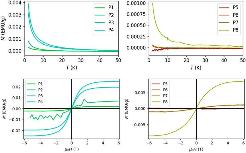
FIGURE 1. Result of Vibrating Sample Magnetometry for free (P1-P4) and clustered (P5-P8) iron samples with concentrations 0.2 mM (samples P1 and P5), 0.4 mM (P2, P6), 0.8 mM (P3, P7) and 1.6 mM (P4, P8). There was an increase in magnetization with decreasing temperature at 0.2T, following the Curie-Weiss law. At a temperature of 2 K, the magnetization of the sample changed with the externally applied magnetic field H. The induced magnetization saturated when H = ±4 T and the relationship could be fitted using a Brillouin function The small reference Gadolinium signal (not shown) has been removed from each curve.

Magnetometry

Magnetometry was performed using a commercially available SQUID magnetometer (MPMS3, Quantum Design GmbH, Darmstadt, Germany). The system was operated in the vibrating sample magnetometry (VSM) mode. Measurements were performed on the samples containing free iron and the iron-clusters with a constant iron-load. The AAS standard iron solution alone was also measured at the two highest concentrations. For each sample, slightly less than 1 g was gently positioned on a thin glass-membrane positioned at mid-height of a cylindrical high purity quartz cuvette, substituting the conventional straw holder. The change in magnetization (2 s averaging) as a function of temperature was measured at 0.2 T (2000 Oerstedt). The temperature was lowered from 300 to 2 K, first at a rate of 50 K/min, and below 250 at 10 K/min. At a temperature of 2 K, the change in magnetization as a function of the applied external field µ₀H between ±6 T was assessed (10 s averaging). The hysteresis curve was fitted with a Brillouin function. The results obtained from the samples total magnetization (expressed in electromagnetic units per Gram, emu/g) was converted from this CGS unit to ppm values in SI units based on the density of the samples obtained with mass-calculation and multiplication with 4π.

MRI acquisition

For scanning at 3 T (Prisma fit, Siemens Healthineers, Erlangen Germany, software: Syngo MR E11), all vials were placed inside a water-filled (0.9% NaCl) cylindrical, ca. 3.2 L plastic (consumer-grade) container (height: 160 mm, diameter: 160 mm). The 2-channel body coil was used for transmission and the 64-channel head/neck coil for image acquisition. After “standard mode” start shim and the acquisition of a localizer image, field-map shimming was performed on the field-of-view (FoV) used for multi-echo gradient-echo 3D imaging (MGRE). Magnitude and phase MGE images were acquired with echo times (TE) from 6 to 42 ms in steps of 6 ms; repetition time (TR) of 53 ms; nominal flip angle (FA) 18°; matrix size of 288 × 288 × 144; FoV of 174 × 174 × 86 mm [3]; acceleration factor (GRAPPA) of 2 and acquisition time (TA) of 14 min 41 sec. Phase images were used for QSM pipeline processing, magnitude images were used for morphological reference. Image reconstruction and coil-combination was performed using the manufacturers standard methods (“adaptive combine” and “Matrix optimization off”).

At 14.1 T (Biospec 141/30, Bruker Corporation, Billerica MA, United States, software: Paravision 360) images were acquired for each vial separately using the standard birdcage volume transmit/receive coil with a diameter of 35 mm. The scanning protocol consisted of 1) global and localized field-map shimming within a cylinder covering the center of the vial; 2) MGRE with TE from 2.5 to 15 m in steps of 2.5 m, TR = 20 m; FA = 10°. The FoV was 20 × 20 × 38.4 mm³ and the matrix (100 × 100 × 192) set to obtain voxel-sizes of 200 µm (TA = 6min24 s); 3) MGRE with an isotropic voxel size of 75 µm (FoV = 19.2 × 19.2 × 38.4 mm³, matrix = 256 × 256 × 512), TE from 3 to 23 in steps of 4 m, TR = 37 m, FA = 10° (TA = 1 h 21 min). For both MGRE sequences, the total read-out bandwidth was kept constant at BW = 100 kHz; 4) a single gradient echo with a FoV of 50 × 19 × 19 mm [3], matrix of 1340 × 512 × 512, yielding a voxel size of ca. 37 μm, acquired at a TE = 17 ms and with TR = 42.85 ms, FA = 12° (TA = 3h12 min), BW = 44.25 kHz; 5) a set of inversion recovery 3D MPRAGE images with voxel size of 200 µm and inversion times TI = 25, 100, 200, 400, 600, 800, 1,000, 1,400, 1800 ms, TR = 2000 ms, FA = 8° (each with TA = 25 min 44 s); 6) multi-slice multi-spin-echo MRI with voxel size 200 µm, TE between 6 and 120 in steps of 6 ms, TR = 1000 ms, same FoV and matrix as for the MPRAGE measurement (TA = 5h7 min); 7) multi-contrast diffusion weighted imaging with voxel size 200 µm, TE = 19 ms, TR = 500 ms and b-values of 50, 100, 300, 600, 1,000, 1500 mm²/s, applied in 6 spatial directions (TA = 3 h). The on-line calculation tool in Paravision 360 was used to generate maps for the apparent diffusion coefficient.

Image analysis

Parametric maps of the longitudinal and effective transverse relaxation rates were fitted with a steepest-descent Levenberg-Marquardt algorithm. R₂* maps were generated by fitting the square of the magnitude signal. R₁ maps were generated voxel-wise from the magnitude data. Fits were performed twice, after determining the TI at which the minimum signal was measured. For the first fit, all data points acquired at TI ≤ TI_min were assigned a negative sign, for the second fit only datapoints below TI_min were assigned a negative sign. The T1-fit that yielded the smallest coefficient-of-variance was chosen for each voxel. T₂ maps were obtained using the extended phase graph modelling as described previously [26].

Quantitative susceptibility maps at 3 T were generated with MEDI+ (http://pre.weill.cornell.edu/mri/pages/qsm.html), as described previously in a multi-centre study [17]. Multi-echo MEDI results were obtained using non-linear analysis of the complex MRI values with the Fit_ppm_complex_TE function [27–29], followed by unwrapping with the region growing algorithm, and background field removal by the projection onto dipole fields (PDF) method [30] prior to application of the morphology enabled dipole inversion algorithm [31], with a lambda value of 1,000. The radius of the kernel used for spherical mean value (SMV) correction was 5.

At 14.1 T the same MEDI pipeline, but without self-referencing and with SMV = 0.5 was used to generate QSM for each separately measured vial (non-linear multi-echo combination). Multi-echo results were also combined according to a linear function, from the B0 field obtained with ROMEO [32] (linear multi-echo combination). Finally, we also evaluated QSM results from single echo images using Laplacian unwrapping followed by RESHARP [33] background removal using Tikhonov regularization with a factor of 10⁻³ prior to dipole inversion with the iLSQR algorithm in STI Suite v3.0 (https://people.eecs.berkeley.edu/∼chunlei.liu/software.html).

For the 3 T data, regions-of-interest were defined using the first echo of the 600 micron images and the applet “volumeSegmenter” available in Matlab version R2021b (v 9.11). For each vial, the paintbrush tool was used to define a circle placed within the vial in the bottom slice, and the active contour tool was used to define a region-of-interest covering each vial. Next, the binary file, containing one where a vial voxel is present and zeros otherwise, was smoothed with a gaussian 10 voxel smoothing kernel, and finally a 50% threshold was used. The so-called “CSF_Mask” (cerebrospinal fluid mask) used for self-referencing in MEDI+ was defined by drawing a polygon at the center of the container, just below the vial holder, followed by the active control tool and the erode tool, with a radius of 10 and 4 iterations. Mean values for the MRI parameters were extracted for each vial and used for further analysis.

For the 14.1 T data, segmentation of clusters was performed in Matlab (R2018b, The MathWorks Inc). The iron-free clusters were identified in the unwrapped and background corrected phase image acquired with a 0.037 mm voxel-size, after gaussian smoothing with sigma = 2 (using function: imgauss3filt) followed by histogram equalization (histeq) and thresholding at 0.97. For the images obtained with 0.2 mm voxels, image-modality dependent signal thresholding was carried out to identify the clusters, as described in Results.

Components of the clusters, connected in 3D, were identified with bwconncomp, considering 26 connected neighbouring voxels (voxels with a shared side or corner), followed by regionprops3 to approximate the size of each cluster by a sphere with the same volume, and obtain the equivalent sphere diameter. Mean values for the MRI parameters were extracted for the clusters and voxels classified as background. The QSM values in the background was used as a reference value for the measurements carried out at 14.1 T.

To evaluate the relationship between the measured parameters (VSM, qMRI parameters, number of clusters found) and the iron concentration in the samples, to determine the molar susceptibility ${\chi }_M$, linear regression analysis was performed using fitlm, and the 95% confidence interval was evaluated with predict in Matlab version R2021a (v 9.10).

To identify voxels where static dephasing and dynamic averaging occurred, the magnitude decay data was fitted voxel-wise by a stretched exponential function [34]:

$S\left(TE\right)=S_0\bullet e^{-\frac{{\left(TE\bullet R_2^{\ast ,eff}\right)}^b}{b}}(1)$

where TE is the echo time, S₀ is the magnitude at a TE = 0, R₂^*,eff is the effective relaxation rate, and b is the stretching factor yielding b = 1 for a mono-exponential function and b = 2 for a Gaussian function. Voxels with b > 1.9 were segmented and assigned to the “static dephasing” category, and voxels with 0.6 < b < 1.4 to the “dynamic averaging” category.

Results

Vibrating sample magnetometry

The change in magnetization with decreasing temperature followed a Curie-Weiss relationship, and the Brillouin function was used to fit the change in magnetization with the external field (Figure 1). The magnetization of free iron was markedly stronger than that of the clustered iron. The magnetization of the samples was saturated at applied magnetic fields of ±4 T.

The iron-solution, which is available as a reference standard for atomic absorption spectroscopy yielded a magnetic moment of 5 ± 0.2µ_B (expressed per iron atom in units of the Bohr magneton, µ_B = 9.274.10⁻²⁴J/T) from the Brillouin function fit, which corresponds well with iron in its Fe³⁺ oxidation form (five electrons in shell 3 days).

The alginate embedding of the phantom material also contained small amounts of Gadolinium (30 µM), with significantly lower influence on the saturation magnetization than iron (60%–1000% lower for free iron and 6%–300% for clustered iron). It was not possible to perfectly disentangle the influence of the two and quantify the magnetic moment of each type of ion. As an estimate, the samples containing free iron had a magnetic moment in the range of about 3–4.5 µ_B, while in the samples containing clustered iron, lower values of ca. 1 µ_B were observed. The data showed a tendency towards a decrease in magnetic moment with increasing iron concentrations.

The total susceptibility in emu/g, measured at the saturation level and converted to the SI-unit ppm for each sample, was used as a global measure of magnetization of the samples containing the phantom materials (Figure 2). The total magnetization increased linearly with iron concentration for the free iron samples, yielding a molar susceptibility of 207 ± 32 ppb mM⁻¹ iron (adjusted coefficient of determination = 0.89, p = 0.00298) and an offset, which was not significantly different from zero (46 ± 33 ppb). Exclusion of the highest iron concentration yielded 326 ± 45 ppb mM⁻¹ iron (adjusted coefficient of determination = 0.946, p = 0.0182) and an offset of 10 ± 22 ppb. The fit for the clustered iron including all concentrations was non-significant, since the magnetization measured for the clusters with the highest iron concentration was lower than at the lower concentrations. Excluding this observation yielded a ${\chi }_M$ of 50.7 ± 8.0 ppb mM⁻¹ iron (adjusted coefficient of determination = 0.929, p = 0.0238) and an offset of 23 ± 4 ppb. One may speculate that at higher concentrations antiferromagnetic coupling occurs within the clusters, which could explain the relatively low magnetization found in the sample with clustered iron. Such a tendency could possibly also be found, since the increase in magnetization measured at the three lowest concentrations was linear, while the magnetization at the highest concentration deviated slightly from predictions based on the lowest three concentrations.

FIGURE 2

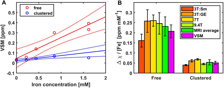
FIGURE 2. Validation of MRI results with vibrating sample magnetometry (VSM) and MRI. (A) VSM susceptibility values of the phantom materials increased linearly with iron concentration for the free iron samples (red), yielding a slope of 207 ± 32 ppb mM⁻¹ iron (adjusted coefficient of determination = 0.89, p = 0.00298). The samples containing clustered iron (blue) at concentrations < 1 mM yielded a linear increase of 50.7 ± 8.0 ppb mM⁻¹ iron (adjusted coefficient of determination = 0.929, p = 0.0238) and an offset of 23 ± 4 ppb. The 95% confidence interval of the linear fits are shown as dotted lines. (B) The results obtained with VSM are compared with the molar susceptibility determined in a multi-centre MRI study [17] where free and clustered iron samples were measured at 3T (Sm, Siemens; GE, General Electrics), 7T and 9.4T. The average across the four scanners compares favourably with the results obtained using VSM.

MRI at 3 T

R₂* and QSM maps were obtained from GRE MRI acquisitions at 3 T using isotropic 0.6 mm voxel sizes and compared for different batches of clustered iron with a 1.6 mM iron concentration and the same iron load (8.3 µg Fe/mg NaPA Figure 3). Batch 1 was used previously in the multi-centre study [17], while Batch 2–4 were made for the present study. The multicentre Batch 1 had homogeneous clusters yielding R₂* values that were similar across voxels (sharper histogram distributions). Batch 2–4 were manufactured after a change of personnel and relative to batch 1, the newer batches had a shift towards higher R₂* and a more than threefold wider distributions of R₂* values. The QSM histograms were more similar across batches, although in the present study Batch 2–4 had a ca. 30% wider distribution and a slightly lower average QSM value than Batch 1. A higher QSM value reflect a stronger coherent shift of the magnetic field within the voxel, and the wider distribution a more prominent field inhomogeneity across the vial. This suggests on the one hand that Batches 2–4 had a more heterogenous distribution of iron, both across and within voxels, and on the other hand, that the batches could be manufactured in a reproducible way.

FIGURE 3

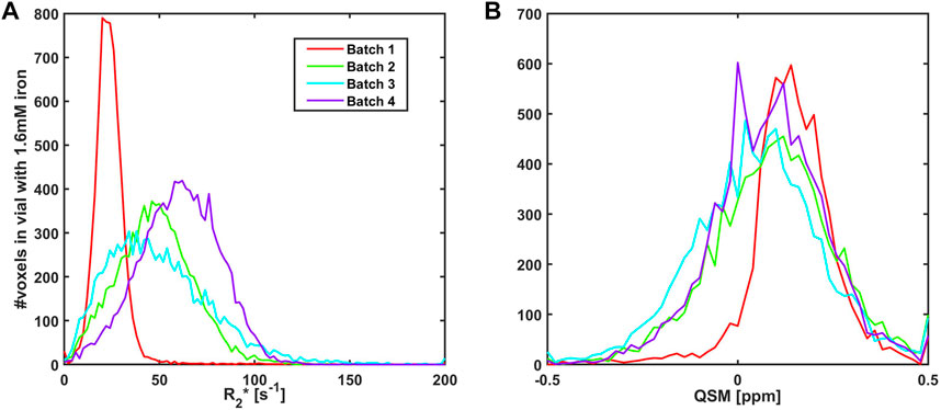
FIGURE 3. Histograms showing the distribution of R₂* (A) and QSM (B) values at 3T using 0.6 mm voxels in vials containing 1.6 mM iron and 120 mg sodium polyacrylate for different batches yielding an iron-load of 8.3 µg Fe/mg NaPA. Batch 1 (solid red line) was used in a previous multi-centre study [17] while the remaining three batches (green, cyan and violet solid lines, Batch 2–4) were manufactured for the present study. Batch 2–4 had similar R₂* distributions that were more than three times wider than for Batch 1, while the range of QSM values was ca. 30% wider than previously.

The vials in Batch 4 had an increasing amount of iron and a fixed amount of polyacrylate (120 mg), while in Batch 2 and 3 each cluster had a fixed iron-to-polyacrylate ratio (of 8.3 µg Fe/mg NaPA). The widths of the QSM histograms were similar at the highest iron concentration while the width of Batch 4 (Figure 4A) was one-third of Batches 2 and 3 for the lowest concentration (Figure 4B). This is consistent with a more homogeneous distribution of iron in presence of large amounts of NaPA, while a non-uniform iron distribution is at hand when iron is accumulated in a few clusters in presence of a fixed iron-to-polyacrylate ratio. In both types of samples, a clear shift towards higher QSM values with increasing iron concentrations was observed (Figures 4C, D). The molar susceptibility was 50.6 ± 11.4 ppb mM⁻¹ for Batch 4 (adjusted coefficient of determination = 0.863, p = 0.0469). This value is in agreement with results obtained previously in presence of clusters with a varying iron load in the multi-centre study, which was 54 ± 13 ppb mM⁻¹ across scanners [17]. With a constant Fe-to-NaPA-ratio and an increasing number of clusters, similar results were obtained for the samples: ${\chi }_M$ = 56.1 ± 6.3 ppb mM⁻¹ iron (adjusted coefficient of determination = 0.963, p = 0.0122).

FIGURE 4

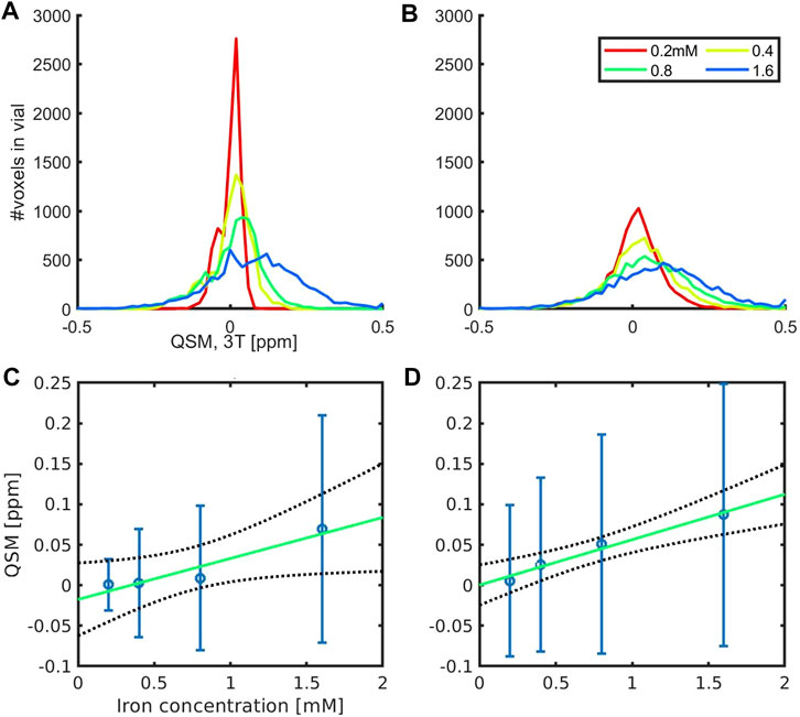
FIGURE 4. QSM histograms (A,B) and molar susceptibility, ${\chi }_M$ (C,D), measured at 3 T for two types of phantoms. In Batch 4 (A,C), an increasing amount of iron and a fixed amount of polyacrylate (120 mg) was used, while in Batch 2 (B,D) a fixed iron-to-polyacrylate ratio (8.3 µg Fe/mg NaPA) was used (B,D). Results for four different iron concentrations: 0.2 mM (solid red line), 0.4 mM (yellow), 0.8 mM (green) and 1.6 mM (blue) are shown. QSM processing was performed with the MEDI + pipeline using zero-referencing to the surrounding water, and a regularization lambda factor of 1000, in agreement with a previous multi-centre study. The average QSM values and within-vial standard deviations are shown for Batch 4 with varying iron-load per cluster (C) and Batch 2 (D) with a constant iron-load. Linear regression analysis yielded a ${\chi }_M$ of 50.6 ± 11.4 ppb mM⁻¹ iron (adjusted coefficient of determination = 0.863, p = 0.0469) and 56.1 ± 6.3 ppb mM⁻¹ iron (adjusted coefficient of determination = 0.963, p = 0.0122), respectively. The 95% confidence intervals for the linear regression analysis are shown as dotted black lines.

MRI at 14.1 T

The samples containing clusters with a constant iron-to-polyacrylate ratio were further characterized by MRI at 14.1 T using different isotropic voxel sizes between 0.037 and 0.2 mm and different qMRI methods.

At the highest resolution, only single echo images with a TE of 17 ms were available (Figure 5). At this TE, the phase images obtained with iron-filled clusters were wrapped multiple times, which could not be perfectly corrected during QSM processing. The iron free clusters stood out as local, slightly more paramagnetic entities compared to the background exhibiting a broad QSM histogram (0.007 ± 0.007 ppm higher). The equivalent sphere diameter of the iron-free clusters estimated in this image series was 276 ± 230 µm.

FIGURE 5

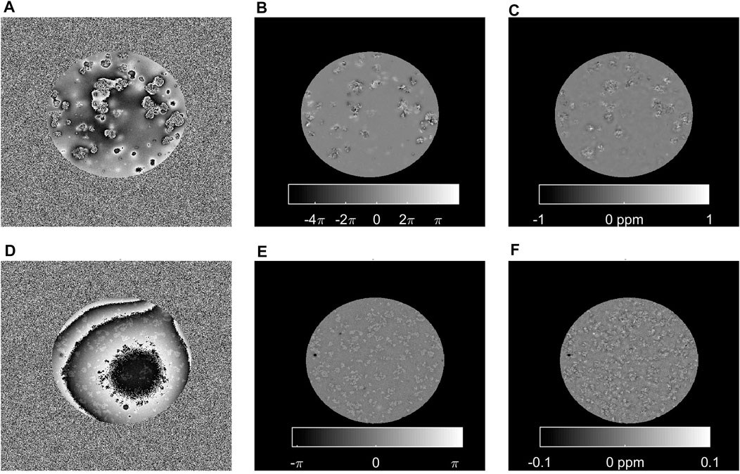
FIGURE 5. Single gradient echo phase and QSM images of samples containing clusters with 0.4 mM iron and 60 mg polyacrylate (A–C) or without iron and 120 mg polyacrylate (D–F). High-resolution (voxel size: 0.037 mm), single echo (TE = 17 ms) MRI was performed at 14.T. The raw phase (A,D), measured at this echo time is wrapped multiple times at the locations of the iron-containing clusters, while no large phase jumps are present in proximity of clusters without iron, although a large background field can be noticed. After unwrapping and background field correction, some uncorrected local field deviations can be discerned (B) resulting in inhomogeneous QSM images (C) for the iron-clusters. On the contrary, in absence of iron, Laplacian unwrapping and RESHARP background field correction reveal small local entities with deviating field (E), corresponding to the iron-free sodium polyacrylate clusters that are more paramagnetic (0.007 ± 0.007 ppm) than the surrounding voxels (F).

With larger voxels of 0.075 mm, the phase images obtained at echo times of 3 ms could be unwrapped, while at 11 ms only the phase images obtained with iron-free samples were completely unwrapped (Figure 6). QSM was obtained with different processing pipelines: single echo analysis, non-linear (MEDI) or linear (ROMEO) multi-echo combination. For the iron-loaded clusters, the unwrapped and background corrected as well as the QSM images looked less blurred at the earlier echo time compared to the later TE where phase unwrapping was incomplete. On the other hand, the weak paramagnetic effect in the iron-free clusters disappeared in the noise at the early TE, and only emerged at the later TE. Non-linear and linear echo combination resulted in QSM results that were comparable to those obtained at the first TE for the iron-loaded clusters, but with reduced noise. For the iron-free clusters, the multi-echo analysis methods yielded results that were similar to the late echo images. The images obtained with MEDI were slightly more eroded, owing to the use of spherical mean value correction.

FIGURE 6

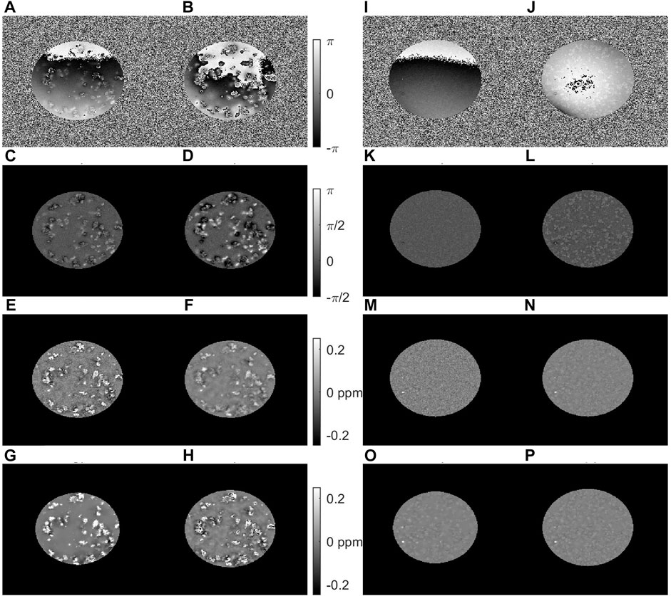
FIGURE 6. Results from multi gradient echo imaging of samples containing clusters with 0.4 mM iron and 60 mg polyacrylate (A–H) or without iron and 120 mg polyacrylate (I–P) measured at 14.1 T with 0.075 mm voxels. The raw phase (A,B) and (I,J), and the phase after Laplacian unwrapping and RESHARP background field correction (c-d, k-l) are shown at TE = 3 ms (A,C,I,K) and TE = 11 ms (B,D,J,L). QSM results for single echo analysis at TE = 3 ms (E,M), and TE = 11 ms (F,N) and multi-echo analysis using nonlinear echo combination in MEDI (G,O) and linear echo-combination in ROMEO (H,P) are shown. Some issues linked with insufficient phase unwrapping in proximity of iron-loaded clusters at the later echo time yield a more blurred appearance of the clusters in the QSM images obtained with single echo analysis, compared to the early echo time and the echo combination methods. In iron-free clusters, the small paramagnetic effect that could be detected at a higher resolution (Figure 5) can still be discerned at the late echo time and after echo-combination.

Similar results were obtained with voxel sizes of 0.2 mm at echo times of 2.5 and 7.5 ms, although the QSM contrast in the iron-free clusters was less prominent even after multi-echo combination (Figure 7).

FIGURE 7

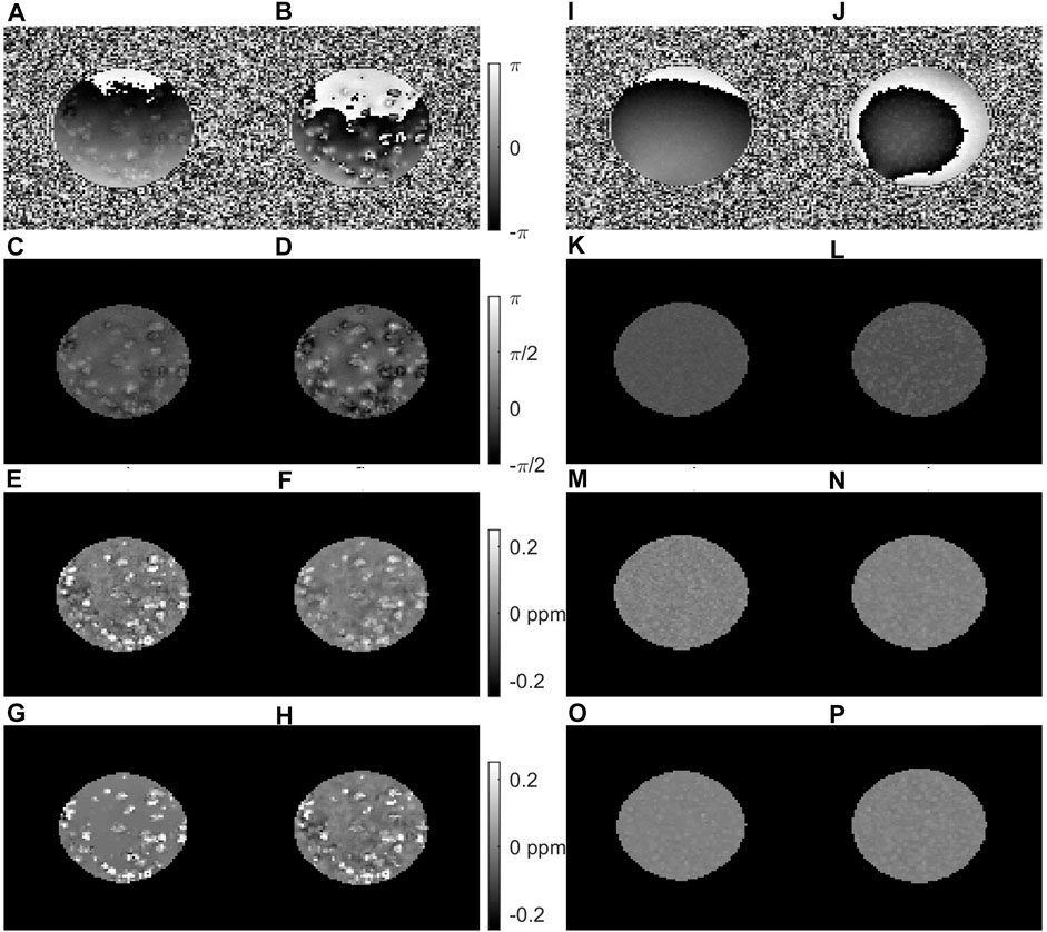
FIGURE 7. Results from multi gradient echo imaging of samples containing clusters with 0.4 mM iron and 60 mg polyacrylate (A–H) or without iron and 120 mg polyacrylate (I–P) measures at 14.1 T with 0.2 mm voxels. The raw phase (A,B) and (I,J), and the phase after Laplacian unwrapping and RESHARP background field correction (C,D,K,L) are shown at TE = 2.5 ms (A,C,I,K) and TE = 7.5 ms (B,D,J,L) with the corresponding QSM results for single echo analysis (E,F,M,N), non-linear MEDI (G,O) and linear ROMEO (H,O) multi-echo combination. Similar to the results obtained with 0.075 voxels (Figure 6), the QSM contrast is suppressed at the later echo time in iron-loaded clusters, while the multi-echo QSM processing pipelines yield similar contrast.

The QSM maps were zero-referenced to the median QSM value found in voxels with a R₂* value below 30 s⁻¹, that were assumed to be iron-free based on the upper bound of the 95% confidence-interval of the R₂* value found for the sample containing iron-free clusters (Table 1). The QSM histograms were symmetric and narrow for MEDI (Figure 8B). With the pipelines based on the first single echo (Figure 8A) and the linear echo combination (Figure 8C) methods, a second peak appeared at high QSM-values. It was particularly prominent for the vial with the highest concentration and for acquisitions with the smaller voxel sizes yielding a larger within-vial standard deviation than with 0.2 mm voxels (Figures 8D–F), indicating that more of the heterogeneity of the phantom material could be assessed at the higher resolution, which allowed local iron clusters to be resolved. Using these 0.075 mm voxels, a QSM-based molar susceptibility of 43.0 ± 0.2 ppb mM⁻¹ (adjusted coefficient of determination = 0.992, p < 0.00257) was obtained with MEDI, and even lower values of 21.8 ± 1.3 and 22.7 ± 1.9 ppb mM⁻¹ with the single echo and the ROMEO-based pipelines, respectively. This discrepancy was mirrored by more well-defined QSM values with narrow distributions for MEDI (Figure 8B).

TABLE 1

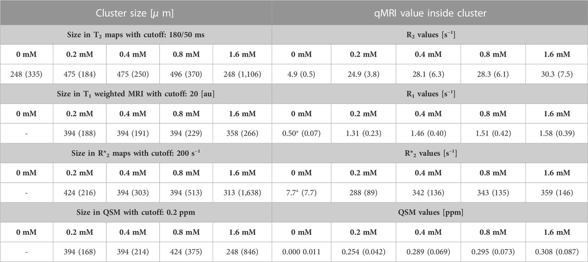
TABLE 1. Size and qMRI values of hydrogel clusters. Clusters were identified on different imaging modalities acquired with an isotropic voxel size of 0.2 mm at 14.1 T. The cluster size (in $\mu$ m) was expressed as the diameter of an equivalent sphere with the same volume as the cluster. The observed average and standard deviation (SD) relaxation rates: R₂, R₁, and R₂* and QSM values (from the first echo) within the segmented clusters are listed for different iron concentrations. ^aThe iron-free clusters could only be reliably segmented in the T₂-maps, therefore the global average within the vial is shown for T₁ and R₂* and QSM. The standard deviations (SD) for the cluster size and the qMRI values are indicated in parentheses.

FIGURE 8

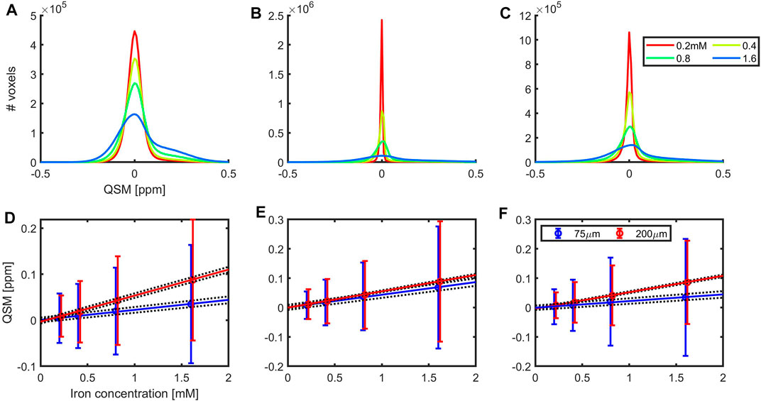
FIGURE 8. QSM histograms of results obtained at 14.1 T with 0.075 mm voxels (A–C) and molar susceptibility (D–F) for vials containing clusters with a fixed iron-to-polyacrylate ratio (8.3 µg Fe/mg NaPA) with iron concentrations of: 0.2 mM (solid red line), 0.4 mM (yellow), 0.8 mM (green) and 1.6 mM (blue). QSM processing was performed with the first single echo (A,D), non-linear MEDI (B,E) or linear ROMEO (C,F) echo combination. The average QSM values and within-vial standard deviations are shown for data acquired with a 0.075 and 0.2 mm voxel size. The ${\chi }_M$ was more similar across voxel-sizes with nonlinear MEDI-based echo combination than with the other two processing pipelines.

With a voxel-size of 0.2 mm, ${\chi }_M$ was more similar to the results obtained previously at 3–9.4 T: 55.6 ± 0.7 ppb mM⁻¹ (adjusted coefficient of determination = 1, p < 0.0001) using MEDI, 56.7 ± 1.0 for the single echo approach and 56.0 ± 0.7 ppb mM⁻¹ for the linear echo combination.

The R₂* relaxivity was substantially smaller with the 0.075 mm voxels: 42.1 ± 0.7 s⁻¹ mM⁻¹ (adjusted coefficient of determination = 0.999, p < 0.0003) than with 0.2 mm: 100.3 ± 0.6 s⁻¹ mM⁻¹ (adjusted coefficient of determination = 1, p < 0.0001). Taken together, these results suggest that at the higher resolution, the within voxel field is more homogeneous. Depending on the QSM pipeline, sub-regions with different iron-concentrations can be separated. The 0.2 mm voxels are of a size similar to the clusters and may work as a matched filter that allows the combined effect of local iron inclusions within the voxel to be assessed. In this situation, comparable results were obtained across QSM-pipelines. The QSM-based ${\chi }_M$ obtained with the non-linear echo combination available with MEDI was less dependent on the voxel size than the other two pipelines.

The relationship between R₂* and QSM values obtained from the multi-echo gradient images with 0.075 and 0.2 mm voxel sizes (Figure 9) was further evaluated on a voxel-by-voxel basis, for different classes of voxels with specific R₂* values. For this purpose, the range of R₂* values between 1 and 501 s⁻¹ were subdivided into 500 bins, and the average QSM value for each bin was extracted. These QSM values reached a plateau for voxels with R₂* values above 200 s⁻¹ regardless of voxel size and processing pipeline. In Figure 10, the high variability of R₂* values within the clusters is illustrated.

FIGURE 9

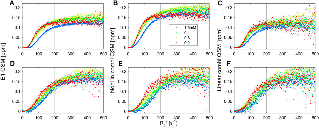
FIGURE 9. Relation between QSM values for voxels with a defined R₂* value between 1 and 501s⁻¹, subdivided into 1 s⁻¹ bins. The images were obtained by multi-echo GRE using 0.075 mm (A–C) and 0.2 mm (D–F) voxel sizes for samples with a fixed iron-to-polyacrylate ratio (8.3 µg Fe/mg NaPA) and a total iron concentration of 0.2 (red dots), 0.4 (green), 0.8 (yellow) or 1.6 mM (blue). QSM values were obtained through single-echo analysis at the first echo time (A,D), and by multi-echo analysis based on nonlinear echo combinations in MEDI (B,E) or by linear echo combination from the field map obtained with ROMEO (C,F). A linear relationship between QSM and R₂* values between 50 and 150 s⁻¹ and a plateau above 200–250 s⁻¹ are found for all iron concentrations, voxel sizes and QSM processing pipelines.

FIGURE 10

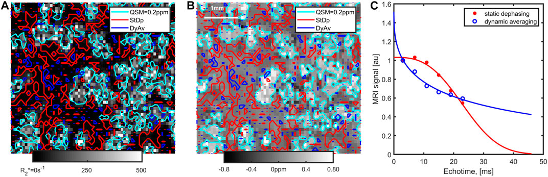
FIGURE 10. Zoomed-in views of the R₂* (A) and MEDI-QSM (B) observed with 0.075 voxels for the sample with 1.6 mM iron. The cyan iso-contour lines for a QSM value of 0.2 ppm are outlined on both images. On the R₂* maps, the large variability in the local R₂* values within the clusters can be noted (cfr Figure 9). Several voxels, mainly located outside the clusters, exhibit static dephasing behaviour, and others show evidence of dynamic averaging, as further evidenced in the (C) time-series showing the average magnitude signal within segmented voxels.

The QSM values at the plateau were similar across iron concentrations, reaching levels of 175–223 ppb for voxels of 0.2 mm, with similar results at 0.075 mm using MEDI. The single echo and ROMEO pipelines yielded lower average QSM values at the plateau (119–158 ppb).

Below the plateau, a linear relationship between the two qMRI parameters was found. To investigate the increase in R₂* for each ppb change in QSM, voxels with a range of R₂* values between 50 and 150 s⁻¹ were selected, yielding an increase of 0.07 ± 0.01 s⁻¹ per Tesla for each ppb of change in the measured susceptibility. This value is slightly lower than for spherical particles in the static dephasing regime for which a value of 0.11 s⁻¹ T⁻¹ ppb⁻¹ iron can be predicted [23, 35]. The diffusion weighted MRI signal decreased according to a monoexponential function and the apparent diffusion coefficient was ca. 1.7 μm²/ms, corresponding to a diffusion length of 5–10 µm for echo-times between 2.5 and 10 ms. In view of the large cluster size, as shown in Figure 5 and analysed in more detail in the next paragraph, one could thus expect that effects caused by static dephasing can be observed. However, the non-uniform spatial distribution of iron within the clusters, and the large voxel-sizes used may impede observation of such effects. Along these lines of thought, we identified voxels that exhibited dynamic averaging and static dephasing effects according to (Eq. 1) (Figure 10). Of these voxels, only 14% or less were located within the clusters, as defined by a 0.2 ppm QSM cut-off value in the MEDI images. Within the clusters, QSM values were similar, while R₂* varied greatly (corresponding with the results in Figure 9). This observation is consistent with an overall shift in the magnetic field, combined with a high (root-mean-squared) variation in the magnetic field within the voxels located inside the clusters. Possibly, these QSM results reflect the saturation effect observed with VSM at the highest iron concentration, caused by locally high levels of iron agglomeration.

Segmentation of clusters and qMRI results with 0.2 mm voxel size

Segmentation of clusters was performed using four different image modalities, acquired with a voxel size of 0.2 mm: quantitative T₂-maps, T₁-weighted MRI, and quantitative R₂*-maps. Since the cluster size can depend on the cut-off used, we chose various cut-offs based on image intensity histograms (Figure 11) observed with the 0.8 mM sample, which had the highest susceptibility in the VSM measurement, and with QSM maps at the plateau values determined in Figure 9. The qMRI values inside the clusters, as well as the cluster size, expressed as the diameter of a sphere with the same volume as the segmented clusters, were determined (Table 1).

FIGURE 11

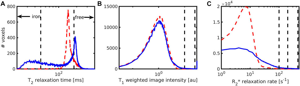
FIGURE 11. Intensity histograms for samples without (0mM, red dashed line) and with (0.8 mM, blue solid line) iron, using three MRI modalities and 0.2 mm voxels measured at 14.1 T. Histograms were obtained from (A) T₂-maps (B) T₁-weighted MPRAGE images with an inversion time of 800 ms; (C) quantitative R₂* maps. The location of the different cut-offs used for segmentation of iron-containing and iron-free clusters are shown as black dashed vertical lines. Note that the iron-free clusters could only be observed in the T₂-maps.

Using the T₂-maps, the hydrogel clusters without iron were segmented as voxels with a T₂ value above 180 m, while iron-containing clusters were identified as voxels with T₂ below 50 m. For reasons of the B₁ (in)homogeneity of the coil used, only the most central slices were analysed (15 slices covering 3 mm along the axial field-of-view). Without iron, the contrast difference between the hydrogel and its surrounding was just about discernible while the iron-loaded clusters showed a stronger contrast difference (Figure 12). The size of the segmented clusters was 248 ± 335 µm, while the iron-loaded clusters appeared larger in the quantitative T₂ images reaching sizes around 500 µm (Table 1). At the highest concentration, the clusters could not be separated well and appeared as a mixture of very small and a few very large clusters. Despite the rather crude 0.2 mm spatial sampling, iron-free clusters had a size that corresponded with the size of 276 ± 230 µm determined using 37 µm voxels (shown in Figure 5).

FIGURE 12

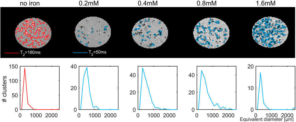
FIGURE 12. Maps (axial view) of the transverse relaxation time, T₂, for samples measured with a voxel size of 200 μm at 14.1 T (upper row). Clusters without iron were identified as voxels with T₂ > 180 ms (red), and clusters with iron T₂ < 50 ms (blue). The corresponding size distributions, expressed as the diameter of a sphere with the same volume as the segmented clusters are shown in the lower row.

A higher number of clusters could be observed in the T₁-weighted images and the R₂*-maps, since good image quality could be obtained across a larger axial field-of-view of 19.2 mm.

In the T₁-weighted image acquired with an inversion time of 800 m, the contrast between iron-loaded clusters and the surrounding was high (Figure 13). The T₁ weighted image and a cut-off of 20 a.u. yielded cluster sizes around 400 µm that were smaller and had smaller standard deviations than in the T₂-map. The number of clusters detected with the highest cut-off value increased linearly, yielding an iron-dependent cluster density of 9.0 mm⁻³ mM⁻¹+1.2 (DoC:0.967, p < 0.0112). Within the segmented clusters there was no change in the longitudinal relaxation rate R₁ with increasing iron concentration.

FIGURE 13

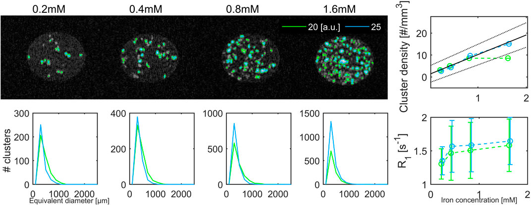
FIGURE 13. T₁-weighted MRI images with an inversion time of 800 ms and a voxel size of 200  μm at 14.1 T. Iron-containing clusters were segmented at two thresholds (20 a.u. green, 25 a.u. blue solid line). The size-distribution for the segmented clusters were similar. The cluster density increased significantly with increasing iron load for clusters segmented with a cut-off of 25 a.u. The corresponding R₁ relaxation rate reached a plateau for iron concentrations of 0.4 mM and above.

Cluster segmentation using the R₂*-maps was performed by thresholding at 100, 200 and 450 s⁻¹ (Figure 14). The average cluster size did not increase significantly with iron concentration and varied largely reaching sizes of 1–1.2 mm because of insufficient separation between clusters. This led to large standard deviations for the cluster size, especially at the highest iron concentration (Table 1). Using the highest cut-off value there was a tendency towards a linear increase in the number of clusters with iron-concentration, yielding a cluster density of: 10 mm⁻³ mM⁻¹+1.3 (DoC:0.814, p < 0.064). At none of the cut-offs, an increase in the R₂* relaxation rate with increasing iron concentrations was found. The same increase in cluster density was obtained from the QSM maps obtained with the linear echo combination and a cut off of 0.4 ppm.

FIGURE 14

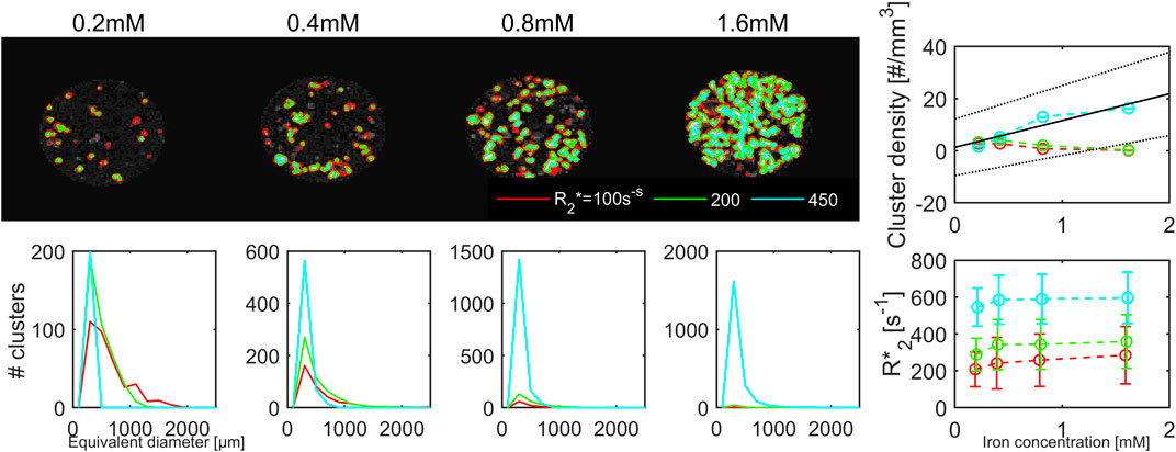
FIGURE 14. Maps of the effective transverse relaxation rate, R₂*, acquired with a voxel size of 200 μm at 14.1 T. Iron-containing clusters were segmented at three thresholds: 100 s⁻¹ (red solid line), 200 s⁻¹ (green) and 450 s⁻¹ (cyan). At the highest threshold there was a tendency for a linear increase in cluster density with increasing iron load. No significant change in R₂* with increasing iron concentrations were observed.

Discussion

The availability of well-characterized phantoms suitable to assess the many factors influencing quantification are fundamental to facilitate clinical use of quantitative MRI methods, but pose some challenges, especially if the aim is to mimic tissue microsctructure [36]. In the case of quantitative susceptibility mapping (QSM) with MRI, such phantoms are of value since many factors, related to the MRI measurement, on one hand, and the processing pipeline on the other hand influence the level of accuracy and precision that can be achieved. The use of tissue-mimicking phantom materials allows to assess the influence of each factor in detail in a setting that should be as realistic as possible, given the complexity of MRI signals arising from the tissue in vivo.

QSM is based on the successful acquisition of high quality phase images, obtained using a fully spoiled gradient-echo MRI sequence. The quality of the phase images depends on the available signal-to-noise ratio in the magnitude images, and therefore on factors like the magnetic field strength at which the measurement is carried out as well as the echo-time and voxel size used for image acquisition. Using MRI, the measured signal phase is assumed to evolve linearly with the echo-time, but the phase values will be aliased into the ±π range during image acquisition. Provided that the range of susceptibility values that will be encountered within the tissue is known, the echo time—or in case of multi-echo sequences: the inter-echo delay time—can be used as a scaling factor to achieve an “adequate” amount of phase aliasing. Just how much aliasing that can be tolerated depends on the type of unwrapping used during QSM processing. Unwrapping [32, 37–42] can go astray if the echo-time is too long and/or if the tissue susceptibility differences are too large, which for instance can happen in presence of local tissue bleedings [41]. Others have reported echo-time dependence of QSM results [43], suggesting the presence of non-linear phase evolution that also may need consideration.

Besides phase unwrapping, unwanted background field components [9, 33, 44–47]need to be removed prior to the final dipole inversion step [20, 48–50] required to obtained the final QSM results. As an alternative, one-step QSM approaches, which utilize combined unwrapping and background removal can be used [51–53]. Other emerging QSM techniques are based on total field inversion [54] and deep learning approaches [55]. Besides the QSM processing pipeline itself, other factors such as the type of coil-combination algorithm [56, 57] or brain-tissue masking method employed [58] can influence quantification [21].

One possibility to assess the influence of such factors is to perform in vivo measurements of healthy subjects and compare the obtained QSM results in different brain regions with expected non-haeme tissue iron concentration. The mathematical expression describing the expected age-dependent increase in tissue iron [18] lends itself well for such comparisons of the measured QSM-contrast in the healthy human brain. A method that quantifies the iron-dependent QSM-contrast $k_{Fe}$, (unit [ppb/[μg/g]) has been made available for the QSM challenge 2016 data and can be adapted for use at individual sites [21, 59]. However, in case of multi-centre studies, such assessments may require that volunteers travel between sites to assure the protocols are comparable. Other issues can arise if several different types of acquisition protocols are to be assessed, since there is an upper limit to the total scan duration, that is, acceptable in vivo, besides issues related to motion during image acquisition. Therefore, a more practical solution to allow informed decisions based on an iterative optimization process to be made, that includes adjustment of each and single step if needed, is the use of adequate phantoms.

Ideally, the phantom material should reflect the complexity of the tissue and have magnetic properties that are comparable to those found in vivo. Today, besides phantoms containing single susceptibility sources [13, 14] more complex mixtures [15], able to mimic more of the complexity present in vivo, are available. In a previous multi-center study, we introduced a phantom for QSM that contains iron (available as a standard for atomic absorption spectroscopy), either in form of a homogeneous solution, “free” iron, or as small iron clusters after absorption of the iron in a hydrogel consisting of sodium polyacrylate [17]. The iron concentrations used for the phantom were about half of those typically found for non-haeme iron in brain tissue in vivo. The average molar susceptibility that was observed across three magnetic field strengths and four scanners was 0.231 ± 0.047 ppm mM⁻¹ and 0.054 ± 0.013 ppm mM⁻¹ for the free and clustered iron, respectively. The QSM contrast of the proposed clustered iron thus corresponded to the ${\chi }_M$ for ferritin with an iron-load of 3000 atoms, and falls within the range of 28–72 ppb mM⁻¹ iron expected for ferritin in the human brain [19–22].

However, in the previous study, validations through magnetometry measurements were lacking. Moreover, details of the clusters, like their size and spatial distribution, had not been obtained, motivating the present work. Another unknown factor was the possibility to manufacture comparable batches of the phantom material. A general feature of the phantom material, that we already had noted in our previous study, is that the spatial distribution of iron clusters can be hard to control during manufacturing but can be assessed “post hoc” in R₂* and QSM images. Therefore, we used MRI at 3 T with identical imaging and QSM processing protocols as in the previous study in order to assess reproducibility. The batches manufactured in the present study had higher R₂* values and showed a higher variability in R₂* across the containing vials than previously. The QSM values, on the other hand, were found to be more similar across different batches. These observations underline the importance of the manufacturing process. The size and the spatial distribution of the iron-loaded regions will likely depend on the details of the mixing of iron-loaded poly-acrylate hydrogel and the alginate matrix. At the moment, this is done manually, which can have some drawbacks with respect to reproducibility. When scaling-up the sample preparation, switching to mechanical mixing (for instance by using higher speed, blade-like stirrers) might help to produce more homogeneous samples.

With regard to stability of the iron clusters, it can be noted that sodium poly-acrylate is a super-absorbent polymer, which can absorb its own mass multiple times (in our case: a volume corresponding to more than 8 times its own weight). This hydrogel has been employed for removal of heavy metal contamination, owing to its anionic carboxylate binding sites [60]. These can coordinate to Fe³⁺ in various configurations at the molecular scale, and thus can stably bind large amounts of iron (15 mM). The reddish-brown colour appearing when mixing the (acidic) iron standard solution with the (basic) poly-acrylate suggests an increase of pH and subsequent formation of hydrolysis and formation of increasingly poorly soluble condensates of (FeOOH)_x aq. up to insoluble Fe(OH)₃. The formation of these larger condensates will further prevent the diffusion of iron out into the alginate matrix. Our previous results [17] were obtained during a 3 months’ time period, during which the phantom was transported between three laboratories across two continents (in a hand-luggage) and kept at room temperature.

Introducing further variability, we decided to compare two types of phantoms: vials containing a variable amount of iron and fixed amount of NaPA on the one hand and a fixed iron-to-polyacrylate ratio, yielding a fixed amount if iron per cluster and an increasing number of clusters, on the other hand. The first type of phantom corresponds to the one used in our previous study [17], while the second type facilitates observation of single clusters. Regardless of these manipulations, the ${\chi }_M$ results observed were comparable with values between 50 and 56 ppb mM⁻¹, provided that the voxel-size used for MRI acquisition was larger than the size of the clusters.

Although a clear, iron-concentration dependent shift in QSM could be observed, it was accompanied by a large standard deviation across the vial, most likely explained by the large susceptibility difference between the clusters and the alginate surrounding. The standard deviation was particularly large in the phantoms where both the amount of iron and alginate were increased, reflecting that when there is no surplus of polyacrylate, the surrounding alginate remains free from iron, at least to a large extent. The difference in susceptibility between the embedding media and the polyacrylate thence lead to large QSM variability. More fine-scaled variability could be captured when using voxel-sizes that were smaller than the clusters at 14.1T, but also led to a suppression of the observed molar susceptibility. Indeed, with 0.075 voxels, the molar susceptibility derived from the entire vial as a region of interest, was very different from that observed at 3T, especially with the single-echo and ROMEO combination approaches, which had wider QSM histograms than MEDI (Figure 8). Only with a voxel-size of 0.2 mm, which approaches the estimated cluster size, the molar susceptibility at 14.1 T became comparable to the values observed at 3 T with a voxel size of 0.6 mm.

Besides average QSM values, quantifying histogram features could furnish additional, clinically relevant parameters, since generally the distribution of QSM values can be large even within selected anatomical regions-of-interest. Recently Lancione et al [61], showed that the distributions of QSM values observed in vivo within iron-containing structures, like the dentate nucleus and the putamen can be quite large (as shown in the Supporting Figure S4 of that publication). These workers report that specific histogram features, like the standard deviation, the 75th and the 90th percentile were useful parameters to distinguish between Parkinsonian and cerebellar multiple system atrophy.

Although we cannot pinpoint the exact cause for the differences between the current and previous batches, one possible contributor may have been differences in the oxygenation state of the iron between batches, besides differences in the actual spatial distribution of the clusters occurring during manufacturing. The exact oxygenation state at hand can change R₂* yielding greater relaxivity values in presence of ferric than ferrous iron [62, 63]. In addition, ferric iron can fall out and yield a reddish colour. Therefore, it is interesting to note that the clusters generated through the addition of sodium polyacrylate to the iron solution could be visually identified as red dots, which were particularly prominent in the vials containing the highest iron concentration. The change in colour could indicate precipitation of iron inside the hydrogel clusters. However, in order to unambiguously determine the oxygenation state, the use of Mössbauer spectroscopy can be envisaged in future studies [64].

In order to further characterize the phantom material, we used vibrating sample magnetometry, which is a highly accurate and precise technique to assess magnetic properties. Notably, magnetometry has been used previously to assess human tissue [65–69]. Through measurements of the magnetization as a function of temperature, and as a function of the external field, both the type of magnetism and the magnetic moment can be identified. VSM of samples containing the pure iron-solution used for manufacturing the phantom was measured and showed the presence of iron with a magnetic moment of approximately 5µ_B, which corresponds to ferric Fe³⁺ iron which has an effective, magnetic moment of 5.92 µ_B²³ when spin-only effects without nuclear couplings are considered.

We furthermore used VSM to ascertain the susceptibility of the phantom material as a whole, since separation of the contributions from the iron and the small amounts of added Gadolinium ions to the alginate embedding was not perfect. The total magnetization of the sample was found to increase linearly with iron concentration, yielding a molar susceptibility of 207 ± 32 ppb mM⁻¹ for the free and 50.7 ± 8.0 ppb mM⁻¹ for the clustered iron. These values compare favourably with our previous observations in the multi-centre study [17]. Interestingly, the measured magnetic moment in the samples containing clustered iron at the highest concentration was below the value predicted based on concentrations below 1 mM. This indicates that the total signal is not simply the sum of all saturated iron magnetic moments. One may speculate that at higher concentrations antiferromagnetic coupling occurs, which could explain the relatively low magnetization observed in the sample with the highest iron concentration. This effect does not necessarily have to be a solid-state phenomenon. Such phenomenon could arise if the iron is strongly bound in the clusters and subregions with different magnetic moment directions are at hand. As antiferromagnetism, via superexchange, is not a rare phenomenon, we would like to suggest that the reduced saturation is caused by a significant fraction of iron, which are antiferromagnetically coupled on a molecular basis. In line with this, qMRI with 0.075 mm voxels showed that QSM saturates within the clusters, while R₂* varied strongly, possibly due to locally high levels of iron with different magnetic moments. Antiferromagnetic coupling has been observed for magnetite composed of highly ordered, alternating ferric and ferrous iron. To better investigate such sub-lattice ordering effects, X-ray diffraction can be performed. Also, ferritin has a highly complex behaviour as observed with magnetometry, allegedly deriving from the presence of superparamagnetism counteracted by anti-ferromagnetic coupling in its core [70]. Antiferromagnetic coupling effects must not necessarily be manifest in our MRI measurements, which were performed at room temperature with long echo-times of a few milliseconds during which diffusion averaging can occur. Therefore, in this respect VSM yielded more precise and detailed information.

Macroscopic MRI properties can be influenced by packing densities. For iron-loaded ferritin aggregated inside liposomes, transverse relaxation occurs at rates in MRI that are 6 times faster than ferritin outside such liposomes [71]. In our previous study using whole-body scanners operating at 3, 7, and 9.4T, we observed an R₂*-related relaxivity which increased linearly with magnetic field strength by 4.00 s⁻¹ mM⁻¹ T⁻¹, albeit with a (non-significant) intercept of 5.61 s⁻¹. From these numbers, one can predict an R₂* relaxivity of 61.6 s⁻¹ mM⁻¹ at 14.1 T. The batches manufactured in the present study reached 100 s⁻¹ mM⁻¹, consistent with a higher packing density than previously attained.

Segmentation using high thresholds yielded maximal R₂* values of 200–500 s⁻¹ within the clusters, which are reminiscent of the range of 155−310 s⁻¹ expected for ferritin at 14.1T, based on an increase in R₂’ of 0.11 s⁻¹ T⁻¹ ppb⁻¹ iron for spherical particles in the static dephasing regime [23]. On the other hand, in a transition zone surrounding the cluster core, R₂* increased as 0.07 ± 0.01 s⁻¹ T⁻¹ ppb⁻¹ iron, suggesting that averaging effects can occur to a certain extent.

At the highest image resolution used, with an isotropic voxel size of 37 µm, the iron-free clusters had a roundish, snow-flake like appearance with a blurred border. Each cluster occupied a volume that corresponded to a sphere with an equivalent diameter of ca. 250 µm, while after iron-loading the size of the clusters increased to 500–600 µm. To avoid the “blooming-effect” of dephased magnetization in gradient echo images, we complemented observations of the cluster size based on R₂* and QSM images with measurements using spin-echo and short-echo time inversion-recovery MRI. Overall, these techniques yielded similar results regarding the cluster size.

Since the amount of the polyacrylate hydrogel always matched the volume of the iron solution added to the samples, we expected each cluster detected to have the same iron-load, and that the cluster density depends on the iron concentration. The result of the image analysis with voxel sizes of 200 µm was in line with this hypothesis but only when high thresholds were used for cluster segmentation. In that case, the cluster density increased with increasing iron concentration. The qMRI parameters observed within the clusters were the same across all samples.

Taken together, these results point towards iron-loaded clusters with molar susceptibility and R₂* values reminiscent of ferritin in vivo. Reproducibility of QSM results across scanners, batches, and phantom types was within 12% and compared well with results using vibrating sample magnetometry. Using 0.2 mm voxel sizes, the clusters could be delineated and separated from the surrounding, while with voxels of 0.075 mm and below, a heterogeneous spatial distribution of iron with saturated QSM values within single clusters emerged. Around the clusters, heterogeneous MRI signal behaviour, with voxels exhibiting static dephasing effects as well as dynamic averaging could be identified. In future studies, it would be of interest to push the spatial resolution further, even more towards the diffusion length to better assess the impact of such local iron inclusions on MRI.

Data availability statement

The raw data supporting the conclusion of this article will be made available by the authors, without undue reservation.

Author contributions

GH: Conceptualization methodology investigation formal analysis software (MRI) writing—original draft, EG: Methodology investigation formal analysis software (VSM) writing—review and editing EC: formal Analysis (MRI 3T) writing—review and editing JE. resources validation writing—review and editing KS: funding acquisition, supervision writing—review and editing. All authors contributed to the article and approved the submitted version.

Funding

We gratefully acknowledge the EU-LACH Grant #16/T01-0118, and ERC Advanced Grant #834940 for supporting this work.

Conflict of interest

The authors declare that the research was conducted in the absence of any commercial or financial relationships that could be construed as a potential conflict of interest.

Publisher’s note

All claims expressed in this article are solely those of the authors and do not necessarily represent those of their affiliated organizations, or those of the publisher, the editors and the reviewers. Any product that may be evaluated in this article, or claim that may be made by its manufacturer, is not guaranteed or endorsed by the publisher.

References

1. Loureiro JR, Himmelbach M, Ethofer T, Pohmann R, Martin P, Bause J, et al. In-vivo quantitative structural imaging of the human midbrain and the superior colliculus at 9.4T. Neuroimage (2018) 177:117–28. doi:10.1016/j.neuroimage.2018.04.071

PubMed Abstract | CrossRef Full Text | Google Scholar

2. Tuzzi E, Balla DZ, Loureiro JRA, Neumann M, Laske C, Pohmann R, et al. Ultra-high field MRI in Alzheimer’s disease: Effective transverse relaxation rate and quantitative susceptibility mapping of human brain in vivo and ex vivo compared to histology. J Alzheimer’s Dis (2020) 73(4):1481–99. doi:10.3233/JAD-190424

CrossRef Full Text | Google Scholar

3. Ghassaban K, Liu S, Jiang C, Haacke EM. Quantifying iron content in magnetic resonance imaging. Neuroimage (2019) 187:77–92. doi:10.1016/j.neuroimage.2018.04.047

PubMed Abstract | CrossRef Full Text | Google Scholar

4. Biondetti E, Rojas-Villabona A, Sokolska M, Pizzini FB, Jäger HR, Thomas DL, et al. Investigating the oxygenation of brain arteriovenous malformations using quantitative susceptibility mapping. Neuroimage (2019) 199:440–53. doi:10.1016/j.neuroimage.2019.05.014

PubMed Abstract | CrossRef Full Text | Google Scholar

5. Hametner S, Endmayr V, Deistung A, Palmrich P, Prihoda M, Haimburger E, et al. The influence of brain iron and myelin on magnetic susceptibility and effective transverse relaxation - a biochemical and histological validation study. Neuroimage (2018) 179:117–33. doi:10.1016/j.neuroimage.2018.06.007

PubMed Abstract | CrossRef Full Text | Google Scholar

6. Stüber C, Morawski M, Schäfer A, Labadie C, Wähnert M, Leuze C, et al. Myelin and iron concentration in the human brain: A quantitative study of MRI contrast. Neuroimage (2014) 93(1):95–106. doi:10.1016/j.neuroimage.2014.02.026

PubMed Abstract | CrossRef Full Text | Google Scholar

7. Wharton S, Bowtell R. Effects of white matter microstructure on phase and susceptibility maps. Magn Reson Med (2015) 73(3):1258–69. doi:10.1002/mrm.25189

PubMed Abstract | CrossRef Full Text | Google Scholar

8. Deistung A, Schweser F, Wiestler B, Abello M, Roethke M, Sahm F, et al. Quantitative susceptibility mapping differentiates between blood depositions and calcifications in patients with glioblastoma. PLoS One (2013) 8(3):e57924. doi:10.1371/journal.pone.0057924

PubMed Abstract | CrossRef Full Text | Google Scholar

9. Schweser F, Atterbury M, Deistung A, Lehr BW, Sommer K, Reichenbach JR. Harmonic phase subtraction methods are prone to B1 background components. Proc Intl Soc Mag Reson Med (2011) 37(9):2657.

Google Scholar

10. Tuzzi E, Loktyushin A, Zeller A, Pohmann R, Christoph L, Scheffler K, et al. Exploration of cortical ß-Amyloid load in Alzheimer’s disease using quantitative susceptibility mapping at 9.4T. Available at: https://www.medrxiv.org/content/10.1101/2022.09.23.22280290v1 (Accessed September 25, 2022).

Google Scholar

11. Langkammer C, Schweser F, Shmueli K, Kames C, Li X, Guo L, et al. Quantitative susceptibility mapping: Report from the 2016 reconstruction challenge. Magn Reson Med (2018) 79(3):1661–73. doi:10.1002/mrm.26830

PubMed Abstract | CrossRef Full Text | Google Scholar

12. Marques JP, Meineke J, Milovic C, Bilgic B, Chan K, Hedouin R, et al. QSM reconstruction challenge 2.0: A realistic in silico head phantom for MRI data simulation and evaluation of susceptibility mapping procedures. Magn Reson Med (2021) 86(1):526–42. doi:10.1002/mrm.28716

PubMed Abstract | CrossRef Full Text | Google Scholar

13. Olsson E, Wirestam R, Lind E. MRI-based quantification of magnetic susceptibility in gel phantoms: Assessment of measurement and calculation accuracy. Radiol Res Pract (2018) 2018:1–13. doi:10.1155/2018/6709525

CrossRef Full Text | Google Scholar

14. Deh K, Kawaji K, Bulk M, Van Der Weerd L, Lind E, Spincemaille P, et al. Multicenter reproducibility of quantitative susceptibility mapping in a gadolinium phantom using MEDI+0 automatic zero referencing. Magn Reson Med (2019) 81(2):1229–36. doi:10.1002/mrm.27410

PubMed Abstract | CrossRef Full Text | Google Scholar

15. Emmerich J, Bachert P, Ladd ME, Straub S. A novel phantom with dia- and paramagnetic substructure for quantitative susceptibility mapping and relaxometry. Phys Med (2021) 88:278–84. doi:10.1016/j.ejmp.2021.07.015

PubMed Abstract | CrossRef Full Text | Google Scholar

16. Reinert A, Morawski M, Seeger J, Arendt T, Reinert T. Iron concentrations in neurons and glial cells with estimates on ferritin concentrations. BMC Neurosci (2019) 20(1):25–14. doi:10.1186/s12868-019-0507-7

PubMed Abstract | CrossRef Full Text | Google Scholar

17. Gustavo Cuña E, Schulz H, Tuzzi E, Biagi L, Bosco P, García-Fontes M, et al. Simulated and experimental phantom data for multi-center quality assurance of quantitative susceptibility maps at 3 T, 7 T and 9.4 T. Phys Med (2023) 110:102590. doi:10.1016/j.ejmp.2023.102590

PubMed Abstract | CrossRef Full Text | Google Scholar

18. Hallgren B, Sourander P. The effect of age on the non-haemin iron in the human brain. J Neurochem (1958) 3(1):41–51. doi:10.1111/j.1471-4159.1958.tb12607.x

PubMed Abstract | CrossRef Full Text | Google Scholar

19. Chai C, Zhang M, Long M, Chu Z, Wang T, Wang L, et al. Increased brain iron deposition is a risk factor for brain atrophy in patients with haemodialysis: A combined study of quantitative susceptibility mapping and whole brain volume analysis. Metab Brain Dis (2015) 30(4):1009–16. doi:10.1007/s11011-015-9664-2

PubMed Abstract | CrossRef Full Text | Google Scholar

20. Schweser F, Deistung A, Lehr BW, Reichenbach JR. Quantitative imaging of intrinsic magnetic tissue properties using MRI signal phase: An approach to in vivo brain iron metabolism? Neuroimage (2011) 54(4):2789–807. doi:10.1016/j.neuroimage.2010.10.070

PubMed Abstract | CrossRef Full Text | Google Scholar

21. Hagberg GE, Eckstein K, Tuzzi E, Zhou J, Robinson S, Scheffler K. Phase-based masking for quantitative susceptibility mapping of the human brain at 9 4T. Magn Reson Med (2022) 88(5):2267–76. doi:10.1002/mrm.29368

PubMed Abstract | CrossRef Full Text | Google Scholar

22. Zheng W, Nichol H, Liu S, Cheng Y-CN, Haacke EM. Measuring iron in the brain using quantitative susceptibility mapping and X-ray fluorescence imaging. Neuroimage (2013) 78:68–74. doi:10.1016/j.neuroimage.2013.04.022

PubMed Abstract | CrossRef Full Text | Google Scholar

23. Duyn JH, Schenck J. Contributions to magnetic susceptibility of brain tissue. NMR Biomed (2017) 30(4):e3546. doi:10.1002/nbm.3546

CrossRef Full Text | Google Scholar

24. Dedman DJ, Treffry A, Candy JM, Taylor GAA, Morris CM, Bloxham CA, et al. Iron and aluminium in relation to brain ferritin in normal individuals and Alzheimer’s-disease and chronic renal-dialysis patients. Biochem J (1992) 287(2):509–14. doi:10.1042/bj2870509

PubMed Abstract | CrossRef Full Text | Google Scholar

25. DiResta GR, Lee J, Arbit E. Measurement of brain tissue specific gravity using pycnometry. J Neurosci Methods (1991) 39(3):245–51. doi:10.1016/0165-0270(91)90103-7

PubMed Abstract | CrossRef Full Text | Google Scholar

26. Hagberg GE, Bause J, Ethofer T, Ehses P, Dresler T, Herbert C, et al. Whole brain MP2RAGE-based mapping of the longitudinal relaxation time at 9.4 T. Neuroimage (2017) 144:203–16. doi:10.1016/j.neuroimage.2016.09.047

PubMed Abstract | CrossRef Full Text | Google Scholar

27. Kressler B, de Rochefort L, Liu T, Spincemaille P, Jiang Q, Wang Y. Nonlinear regularization for per voxel estimation of magnetic susceptibility distributions from MRI field maps. IEEE Trans Med Imaging (2010) 29(2):273–81. doi:10.1109/TMI.2009.2023787

PubMed Abstract | CrossRef Full Text | Google Scholar

28. Bernstein MA, Grgic M, Brosnan TJ, Pelc NJ. Reconstructions of phase contrast, phased array multicoil data. Magn Reson Med (1994) 32(3):330–4. doi:10.1002/mrm.1910320308

PubMed Abstract | CrossRef Full Text | Google Scholar

29. de Rochefort L, Brown R, Prince MR, Wang Y. Quantitative MR susceptibility mapping using piece-wise constant regularized inversion of the magnetic field. Magn Reson Med (2008) 60(4):1003–9. doi:10.1002/mrm.21710

PubMed Abstract | CrossRef Full Text | Google Scholar

30. Liu T, Khalidov I, de Rochefort L, Spincemaille P, Liu J, Tsiouris AJ, et al. A novel background field removal method for MRI using projection onto dipole fields (PDF): Improved background field removal method using PDF. NMR Biomed (2011) 24(9):1129–36. doi:10.1002/nbm.1670

PubMed Abstract | CrossRef Full Text | Google Scholar

31. Liu J, Liu T, de Rochefort L, Ledoux J, Khalidov I, Chen W, et al. Morphology enabled dipole inversion for quantitative susceptibility mapping using structural consistency between the magnitude image and the susceptibility map. Neuroimage (2012) 59(3):2560–8. doi:10.1016/j.neuroimage.2011.08.082

PubMed Abstract | CrossRef Full Text | Google Scholar

32. Dymerska B, Eckstein K, Bachrata B, Siow B, Trattnig S, Shmueli K, et al. Phase unwrapping with a rapid opensource minimum spanning tree algorithm (ROMEO). Magn Reson Med (2021) 85(4):2294–308. doi:10.1002/mrm.28563

PubMed Abstract | CrossRef Full Text | Google Scholar

33. Sun H, Wilman AH. Background field removal using spherical mean value filtering and Tikhonov regularization. Magn Reson Med (2014) 71(3):1151–7. doi:10.1002/mrm.24765

PubMed Abstract | CrossRef Full Text | Google Scholar

34. Blümich B, Perlo J, Casanova F. Mobile single-sided NMR. Prog Nucl Magn Reson Spectrosc (2008) 52(4):197–269. doi:10.1016/j.pnmrs.2007.10.002

CrossRef Full Text | Google Scholar

35. Yablonskiy DA, Haacke EM. Theory of NMR signal behavior in magnetically inhomogeneous tissues: The static dephasing regime. Magn Reson Med (1994) 32(6):749–63. doi:10.1002/mrm.1910320610

PubMed Abstract | CrossRef Full Text | Google Scholar

36. Fieremans E, Lee H. Physical and numerical phantoms for the validation of brain microstructural MRI: A cookbook. Neuroimage (2018) 182:39–61. doi:10.1016/j.neuroimage.2018.06.046

PubMed Abstract | CrossRef Full Text | Google Scholar

37. Schofield MA, Zhu Y. Fast phase unwrapping algorithm for interferometric applications. Opt Lett (2003) 28(14):1194–6. doi:10.1364/ol.28.001194

PubMed Abstract | CrossRef Full Text | Google Scholar

38. Cusack R, Papadakis N. New robust 3-D phase unwrapping algorithms: Application to magnetic field mapping and undistorting echoplanar images. Neuroimage (2002) 16(3):754–64. doi:10.1006/nimg.2002.1092

PubMed Abstract | CrossRef Full Text | Google Scholar

39. Karsa A, Shmueli K. Segue: A speedy rEgion-growing algorithm for unwrapping estimated phase. IEEE Trans Med Imaging (2019) 38(6):1347–57. doi:10.1109/TMI.2018.2884093

PubMed Abstract | CrossRef Full Text | Google Scholar

40. Eckstein K, Dymerska B, Bachrata B, Bogner W, Poljanc K, Trattnig S, et al. Computationally efficient combination of multi-channel phase data from multi-echo acquisitions (ASPIRE). Magn Reson Med (2018) 79(6):2996–3006. doi:10.1002/mrm.26963

PubMed Abstract | CrossRef Full Text | Google Scholar

41. Cronin MJ, Wang N, Decker KS, Wei H, Zhu W-Z, Liu C. Exploring the origins of echo-time-dependent quantitative susceptibility mapping (QSM) measurements in healthy tissue and cerebral microbleeds. Neuroimage (2017) 149:98–113. doi:10.1016/j.neuroimage.2017.01.053

PubMed Abstract | CrossRef Full Text | Google Scholar

42. Robinson S, Schödl H, Trattnig S. A method for unwrapping highly wrapped multi-echo phase images at very high field: Umpire. Magn Reson Med (2014) 72(1):80–92. doi:10.1002/mrm.24897

PubMed Abstract | CrossRef Full Text | Google Scholar

43. Sood S, Urriola J, Reutens D, O’Brien K, Bollmann S, Barth M, et al. Echo time-dependent quantitative susceptibility mapping contains information on tissue properties. Magn Reson Med (2017) 77(5):1946–58. doi:10.1002/mrm.26281

PubMed Abstract | CrossRef Full Text | Google Scholar

44. Özbay PS, Deistung A, Feng X, Nanz D, Reichenbach JR, Schweser F. A comprehensive numerical analysis of background phase correction with V-SHARP. NMR Biomed (2017) 30(4):e3550. doi:10.1002/nbm.3550

CrossRef Full Text | Google Scholar

45. Gulani V, Calamante F, Shellock FG, Kanal E, Reeder SB. Gadolinium deposition in the brain: Summary of evidence and recommendations. Lancet Neurol (2017) 16(7):564–70. doi:10.1016/S1474-4422(17)30158-8

PubMed Abstract | CrossRef Full Text | Google Scholar

46. Li W, Wu B, Liu C. Quantitative susceptibility mapping of human brain reflects spatial variation in tissue composition. Neuroimage (2011) 55(4):1645–56. doi:10.1016/j.neuroimage.2010.11.088

PubMed Abstract | CrossRef Full Text | Google Scholar

47. Zhou D, Liu T, Spincemaille P, Wang Y. Background field removal by solving the Laplacian boundary value problem. NMR Biomed (2014) 27(3):312–9. doi:10.1002/nbm.3064

PubMed Abstract | CrossRef Full Text | Google Scholar

48. Zheng W, Nichol H, Liu S, Cheng YN, Haacke EM. Measuring iron in the brain using quantitative susceptibility mapping and X-ray fluorescence imaging. Neuroimage (2013) 78:68–74. doi:10.1016/j.neuroimage.2013.04.022

PubMed Abstract | CrossRef Full Text | Google Scholar

49. Shmueli K, de Zwart JA, van Gelderen P, Li T-Q, Dodd SJ, Duyn JH. Magnetic susceptibility mapping of brain tissue in vivo using MRI phase data. Magn Reson Med (2009) 62(6):1510–22. doi:10.1002/mrm.22135

PubMed Abstract | CrossRef Full Text | Google Scholar

50. Liu T, Wisnieff C, Lou M, Chen W, Spincemaille P, Wang Y. Nonlinear formulation of the magnetic field to source relationship for robust quantitative susceptibility mapping. Magn Reson Med (2013) 69(2):467–76. doi:10.1002/mrm.24272

PubMed Abstract | CrossRef Full Text | Google Scholar

51. Sun H, Ma Y, MacDonald ME, Pike GB. Whole head quantitative susceptibility mapping using a least-norm direct dipole inversion method. Neuroimage (2018) 179:166–75. doi:10.1016/j.neuroimage.2018.06.036

PubMed Abstract | CrossRef Full Text | Google Scholar

52. Liu Z, Kee Y, Zhou D, Wang Y, Spincemaille P. Preconditioned total field inversion (TFI) method for quantitative susceptibility mapping. Magn Reson Med (2017) 78(1):303–15. doi:10.1002/mrm.26331

PubMed Abstract | CrossRef Full Text | Google Scholar

53. Langkammer C, Bredies K, Poser BA, Barth M, Reishofer G, Fan AP, et al. Fast quantitative susceptibility mapping using 3D EPI and total generalized variation. Neuroimage (2015) 111:622–30. doi:10.1016/j.neuroimage.2015.02.041

PubMed Abstract | CrossRef Full Text | Google Scholar

54. Wen Y, Spincemaille P, Nguyen T, Cho J, Kovanlikaya I, Anderson J, et al. Multiecho complex total field inversion method (mcTFI) for improved signal modeling in quantitative susceptibility mapping. Magn Reson Med (2021) 86(4):2165–78. doi:10.1002/mrm.28814

PubMed Abstract | CrossRef Full Text | Google Scholar

55. Jung W, Bollmann S, Lee J. Overview of quantitative susceptibility mapping using deep learning: Current status, challenges and opportunities. NMR Biomed (2022) 35(4):e4292. doi:10.1002/nbm.4292

PubMed Abstract | CrossRef Full Text | Google Scholar

56. Bollmann S, Robinson SD, O’Brien K, Vegh V, Janke A, Marstaller L, et al. The challenge of bias-free coil combination for quantitative susceptibility mapping at ultra-high field. Magn Reson Med (2018) 79(1):97–107. doi:10.1002/mrm.26644

PubMed Abstract | CrossRef Full Text | Google Scholar

57. Hagberg GE, Eckstein K, Cuna E, Robinson S, Scheffler K. Towards robust QSM in cortical and sub-cortical regions of the human brain at 9.4T: Influence of coil combination and masking strategies. Proc Intl Soc Mag Reson Med (2020) 28:3786.

Google Scholar

58. Schweser F, Robinson SD, de Rochefort L, Li W, Bredies K. An illustrated comparison of processing methods for phase MRI and QSM: Removal of background field contributions from sources outside the region of interest. NMR Biomed (2017) 30(4):e3604. doi:10.1002/nbm.3604

CrossRef Full Text | Google Scholar

59. Hagberg GE. PhasMask4QSM (2022). Available at: https://github.com/ghagberg/PhaseMask4QSM.

Google Scholar

60. Baigorri R, García-Mina JM, González-Gaitano G. Supramolecular association induced by Fe(III) in low molecular weight sodium polyacrylate. Colloids Surf A Physicochem Eng Asp (2007) 292(2-3):212–6. doi:10.1016/j.colsurfa.2006.06.027

CrossRef Full Text | Google Scholar

61. Lancione M, Cencini M, Costagli M, Donatelli G, Tosetti M, Giannini G, et al. Diagnostic accuracy of quantitative susceptibility mapping in multiple system atrophy: The impact of echo time and the potential of histogram analysis. Neuroimage Clin (2022) 34:102989. doi:10.1016/j.nicl.2022.102989

PubMed Abstract | CrossRef Full Text | Google Scholar

62. Dietrich O, Levin J, Ahmadi S-A, Plate A, Reiser MF, Bötzel K, et al. MR imaging differentiation of Fe2+ and Fe3+ based on relaxation and magnetic susceptibility properties. Neuroradiology (2017) 59(4):403–9. doi:10.1007/s00234-017-1813-3

PubMed Abstract | CrossRef Full Text | Google Scholar

63. Birkl C, Birkl-Toeglhofer AM, Kames C, Goessler W, Haybaeck J, Fazekas F, et al. The influence of iron oxidation state on quantitative MRI parameters in post mortem human brain. Neuroimage (2020) 220:117080. doi:10.1016/j.neuroimage.2020.117080

PubMed Abstract | CrossRef Full Text | Google Scholar

64. Papaefthymiou GC. The Mössbauer and magnetic properties of ferritin cores. Biochim Biophys Acta - Gen Subj (2010) 1800(8):886–97. doi:10.1016/j.bbagen.2010.03.018

CrossRef Full Text | Google Scholar

65. Birkl C, Langkammer C, Krenn H, Goessler W, Ernst C, Haybaeck J, et al. Iron mapping using the temperature dependency of the magnetic susceptibility. Magn Reson Med (2015) 73(3):1282–8. doi:10.1002/mrm.25236

PubMed Abstract | CrossRef Full Text | Google Scholar

66. Sharma SD, Fischer R, Schoennagel BP, Nielsen P, Kooijman H, Yamamura J, et al. MRI-based quantitative susceptibility mapping (QSM) and R2* mapping of liver iron overload: Comparison with SQUID-based biomagnetic liver susceptometry. Magn Reson Med (2017) 78(1):264–70. doi:10.1002/mrm.26358

PubMed Abstract | CrossRef Full Text | Google Scholar

67. Kumar P, Bulk M, Webb A, van der Weerd L, Oosterkamp TH, Huber M, et al. A novel approach to quantify different iron forms in ex-vivo human brain tissue. Sci Rep (2016) 6(1):38916. doi:10.1038/srep38916

PubMed Abstract | CrossRef Full Text | Google Scholar

68. Brem F, Hirt AM, Winklhofer M, Frei K, Yonekawa Y, Wieser HG, et al. Magnetic iron compounds in the human brain: A comparison of tumour and hippocampal tissue. J R Soc Interf (2006) 3(11):833–41. doi:10.1098/rsif.2006.0133

CrossRef Full Text | Google Scholar

69. Svobodova H, Kosnáč D, Tanila H, Wagner A, Trnka M, Vitovič P, et al. Iron–oxide minerals in the human tissues. BioMetals (2020) 33(1):1–13. doi:10.1007/s10534-020-00232-6

PubMed Abstract | CrossRef Full Text | Google Scholar

70. Brooks RA, Vymazal J, Goldfarb RB, Bulte JWM, Aisen P. Relaxometry and magnetometry of ferritin. Magn Reson Med (1998) 40(2):227–35. doi:10.1002/mrm.1910400208

PubMed Abstract | CrossRef Full Text | Google Scholar

71. Wood JC, Fassler JD, Meade T. Mimicking liver iron overload using liposomal ferritin preparations. Magn Reson Med (2004) 51(3):607–11. doi:10.1002/mrm.10735

PubMed Abstract | CrossRef Full Text | Google Scholar