Using phase interference to characterize dynamic properties—a review of constant gradient, portable magnetic resonance methods

Spatially resolved motion-sensitized magnetic resonance (MR) is a powerful tool for studying the dynamic properties of materials. Traditional methods involve using large, expensive equipment to create images of sample displacement by measuring the spatially resolved MR signal response to time-varying magnetic field gradients. In these systems, both the sample and the stress applicator are typically positioned inside a magnet bore. Portable MR instruments with constant gradients are more accessible, with fewer limitations on sample size, and they can be used in industrial settings to study samples under deformation or flow. We propose a view in which the well-controlled sensitive region of a magnet array acts as an integrator, with the velocity distribution leading to phase interference in the detected signal, which encodes information on the sample’s dynamic properties. For example, in laminar flows of Newtonian and non-Newtonian fluids, the velocity distribution can be determined analytically and used to extract the fluid’s dynamic properties from the MR signal magnitude and/or phase. This review covers general procedures, practical considerations, and examples of applications in dynamic mechanical analysis and fluid rheology (viscoelastic deformation, laminar pipe flows, and Couette flows). Given that these techniques are relatively uncommon in the broader magnetic resonance community, this review is intended for both advanced NMR users and a more general physics/engineering audience interested in rheological applications of NMR.

1 Introduction

Magnetic resonance (MR) is one of the most powerful, versatile, and safe non-invasive measurement techniques. The best-known implementation is in the clinical use of magnetic resonance imaging (MRI) [1], but other scientific fields, such as material science, have also benefited from MR applications. Magnetic resonance offers a unique combination of features such as non-invasiveness, lack of directional preference, the ability to characterize opaque samples, and the ability to encode multiple parameters in a single measurement. These unique advantages have motivated material science applications of MR techniques that even predate the invention of MRI [2–4].

Quantitative assessment of properties that describe how a material responds to dynamic stress (dynamic properties) is relevant to a variety of industrial and biomedical applications. As a consequence, there has been extensive research into motion-encoding MR techniques. Conventional techniques often employ time-varying gradient waveforms to sensitize the phase of the MR signal to motion, allowing for spatially resolved measurements of motion [5–7]. Theoretical models and computational methods can then be employed to provide quantitative, spatially resolved measurements of dynamic properties.

The above approach has seen applications in several fields, covering industrial and biomedical applications. In magnetic resonance elastography (MRE) [8], elasticity maps (elastograms) can be used as an analog to palpation to differentiate between healthy and unhealthy tissues in the diagnosis and prognosis of a plethora of health conditions [9–12]. In rheological magnetic resonance (Rheo-NMR) velocity maps can be used to gain insight into the behaviours of complex fluids in a variety of flow regimes relevant to industrial processes [13–17].

Despite its remarkable utility, MRI has some limitations that have restricted the range of potential applications. Required instrumentation is typically large, expensive, constrained to a laboratory setting, and imposes restrictions on sample size. Moreover, the technical sophistication required to appropriately implement imaging methods is often broadly inaccessible to the end user.

In recent decades, there has been a concerted effort to develop more accessible, portable MR sensors [18, 19]. Although fundamentally based on the same phenomena, conventional MRI and portable MR methods differ in many ways including the instrumentation employed, the information provided, and the applications targeted. Portable MR instruments are not meant to compete with existing applications of conventional MRI scanners; instead, they aim to bring the fundamental advantages of MR to novel applications in fields where the implementation of conventional systems is impractical, or even impossible.

At this point, it is important to define the word “portable” in the context of this paper and our research. Many instruments have been designed that can be considered more portable than conventional MR spectrometers [20–23]. While impressive achievements in their own right, the use of these instruments is outside the scope of this review. Instead, we will focus on describing methods that have been developed for use with compact (often handheld) arrays consisting of multiple permanent magnets. Given their relative ease of construction, the geometries and magnetic field profiles of portable MR instruments are often designed and optimized to target a specific application or class of applications. For example, constant gradient magnet arrays are commonly employed in motion encoding applications [24–26]. In the early stages of development, the primary objective is to provide a well-rounded description of the experimental parameters; therefore, no attempts are made at improving the portability of accompanying electronics such as RF amplifiers and MR consoles.

In motion encoding applications, the design of a portable MR instrument is typically optimized so that the gradient in the direction of motion dominates over gradients in the orthogonal directions. The strength and uniformity of the gradient required depend strongly on the geometry of the sample, and the range of velocities to be measured. The design of a portable MR instrument must consider several competing factors and their influence on motion sensitivity and signal-to-noise ratio (SNR).

Depending on the instrument, several techniques can be employed to encode motion in the MR signal. Time of flight methods can be used if a considerable portion of the excited sample flows in or out of the sensitive region during the time of acquisition [27–29]. This limits either the velocity or the slice thickness (which is inversely proportional to the RF pulse duration and magnetic field gradient strength [30]).

In net-phase approaches [3, 4, 31], the relative phase of the MR signal contains contributions from successive moments of the magnetic field gradient. Gradient moments (see Section 2.2.2) can be manipulated to encode position, velocity, acceleration, and higher-order terms. Net-phase methods employing portable MR instruments can fail, especially when velocities are non-uniformly distributed throughout the sensitive volume, resulting in phase interference and modulation of signal magnitude, and a loss of phase sensitivity. Some techniques—such as the portable MR flowmeter of [32] - attempt to eliminate phase interference by utilizing a custom flow cell to eliminate wall effects. In this review, we focus on techniques that instead exploit phase interference by encoding dynamic properties using the net-phase accumulation and/or the attenuation of signal magnitude.

As a result of relying on a 1D constant gradient, phase interference-based techniques do not provide detailed spatially resolved information (the most they can provide is a 1D profile); instead, the finite sensitive volume serves as an integrator and encodes information on the spatial distribution of velocities present in the sensitive volume. Changes in the applied stress, or in the dynamic properties of a sample lead to changes in the phase distribution and modulation of the MR signal. We have structured this review to provide detailed descriptions of phase interference techniques from a variety of perspectives by following several example experiments. Each section aims to emphasize a different facet of portable MR phase interference-based techniques by outlining several different experimental perspectives. Given that these techniques are relatively uncommon in the broader magnetic resonance community, this review is intended for both advanced NMR users and a more general physics/engineering audience. Sections detailing MR acquisition procedures and analysis as well as sections detailing NMR fundamentals can be skipped without loss of continuity depending on the experience of the reader.

First, we will outline general theoretical concepts that are fundamental to the MR signal analysis in all experiments. We will establish the versatility of phase interference-based methods by expanding the general analysis into more specific applications such as longitudinal and shear wave elastometry [33, 34], and laminar pipe and Couette flow of non-Newtonian fluids [35, 36].

Subsequently, we will demonstrate the accessibility of portable MR phase interference-based methods by describing the similarities and differences between the instrumentation and acquisition sequences employed in each experiment. We will show how compact, portable magnet arrays and fundamental acquisition schemes can be adapted to analyze motion in a wide range of applications with relative ease.

Next, we will present excerpts of results from each of the example experiments. The validity of phase-interference-based techniques will be established by demonstrating that portable MR instruments can be used to make relative and absolute measurements of dynamic properties. Finally, we will provide an outlook on potential future experiments and applications.

2 Background/theory

2.1 Phase interference of MR signal

Various publications have established the basis for the portable MR phase-interference-based methods discussed in this review. The influence of fluid motion, and by extension, phase interference on spin-echo images has been investigated using conventional imaging methods [37]. This work aimed to separate the effects of shear from other motion artefacts and observed decreases in MR signal within individual voxels; however, this information was not used to extract information on the sample’s dynamic properties. The effects of inhomogeneous B₀ and B₁ magnetic fields (typically the case with portable MR) on the MR signal generated by various pulse sequences have also been studied [38]. While this—like the techniques outlined in this review—describes a bulk measurement, it does not analyze the effects of sample motion, and the analysis provided is for a static sample. The portable MR phase-interference techniques discussed in this paper combine these elements, analyzing the MR signal response to sample motion in a single sensitive region subjected to an inhomogeneous magnetic field.

This section establishes some of the basic MR concepts needed to understand the phase interference idea. For a more rigorous description, one can refer to one of the many reference texts on the fundamentals of magnetic resonance [39, 40]. If the reader is experienced with NMR, this section can be skipped without loss of continuity. Consider the finite sensitive volume of an MR sensor occupied by a large number of nuclei (in most cases hydrogen). Each nucleus has angular momentum and a magnetic dipole moment, the vector average of which results in a net magnetization vector oriented parallel to the background magnetic field, $B_0\widehat{z}$. The B₀ magnetic field exerts a torque on the net magnetization vector, causing it to precess about the z-axis at a position-dependent frequency determined by the Larmor equation,

$\omega \left(\mathbf{r}\right)=-\gamma \left(B_0+\mathbf{r}\cdot \mathbf{G}\right)(1)$

where γ is the gyromagnetic ratio $(\frac{{\gamma }_H}{2\pi }=42.58$ MHz/T), r is the position, and G is the magnetic field gradient. In this context, we are only interested in the variation of the z-component of the magnetic field and define G as follows,

$\mathbf{G}=\vec{\nabla }{B}_z=\frac{\partial B_z}{\partial x}\widehat{x}+\frac{\partial B_z}{\partial y}\widehat{y}+\frac{\partial B_z}{\partial z}\widehat{z}(2)$

Therefore, each nucleus has its own characteristic frequency which contributes to the detected MR signal. With a large number of nuclei present in a finite-sized sensitive volume, the detected signal is a summation of signal contributions from each nucleus and can be expressed as an integral over the dimension of the sensitive volume,

$S={\int }_V\rho \left(\mathbf{r}\right)e^{-i\varphi \left(\mathbf{r},t\right)}dV(3)$

where ρ(r) is the density of excited spins at position r. ϕ(r, t) is the instantaneous phase dependent on the motion of the nuclei and changing magnetic field gradient after the initial excitation of the sample with a radiofrequency pulse (typically 90°). The total phase accumulated after a given time can be determined by integration as follows [41],

$\varphi \left(\vec{r}\right)=\gamma \int \mathbf{G}\left(\vec{r},t\right)\cdot \mathbf{r}\left(t\right)dt(4)$

The portable MR methods described in this review rely on constant magnetic field gradients, both in space and in time. Considering a gradient aligned with motion in the x-direction, the phase can be expressed as,

$\varphi \left(x\right)=\gamma G_x\int x\left(t\right)dt(5)$

Therefore, with some knowledge of the nature of the motion within the sensitive volume, we can predict how the MR signal will respond. In this section, we will expand on these general concepts to develop the analysis using several example experiments with applications in elastometry (characterizing viscoelasticity) and rheometry (characterizing flow). In each case, the effects of phase interference manifest in different ways and thus, require different techniques for the acquisition and analysis of the MR signal.

The example experiments cover cases with minimal phase interference (longitudinal waves) where only net-phase accumulation is used, partial phase interference (laminar pipe flow) where both phase and magnitude are used, complete phase interference (laminar Couette flow) where only magnitude is used, and phase interference that depends on experimental parameters (shear waves) where phase and/or magnitude can be used. Extension of the same fundamental concept to a wide range of physical situations aims to establish the versatility of portable MR phase interference-based techniques.

2.2 Elastometry

The use of magnetic resonance methods in characterizing the viscoelastic properties of materials is well-established in a class of techniques commonly referred to as magnetic resonance elastography (MRE). The conventional approach to an MRE measurement involves synchronizing phase-contrast MR sequences with time-varying harmonic stress waveforms [42]. Tissue displacements are typically induced actively using external sources such as pneumatic, piezoelectric, or acoustic actuators [43]. Most MRE sequences employ time-varying motion-encoding gradient waveforms synchronized with harmonic waveforms to acquire spatially encoded measurements of phase. 2D phase fields are then converted into displacement fields which—through the use of theoretical models [44] and inversion techniques [45–47]—generate images (or elastograms) that display tissue viscoelasticity. Elastograms depict relative differences in the viscoelastic properties of a tissue which serve as biomarkers for a plethora of health conditions in organs such as the liver [48–51], kidneys [52–54], heart [55, 56], brain [57–60], skeletal muscle [61, 62], beast [63, 64], and prostate [65–67].

While conventional MRE techniques can provide useful diagnostic information, they typically require sophisticated acquisition and processing schemes and additional modifications to existing MRI scanners. Naturally, one might wonder if this added complexity is really necessary for every application. Or, are there some applications that might be suited to measurements provided by portable MR methods? This question provides the motivation and potential long-term benefit of developing portable MRE methods. However, some core features of portable MR methods must be emphasized to narrow the focus of possible applications.

The phase interference method—in which the sensitive region of a constant gradient magnet array is used as an integrator to encode motion—by its nature, provides a bulk measurement from a finite region of interest. Therefore, the acquisition of spatially resolved displacement fields is impossible without additional complexity such as time-varying magnetic field gradients. Furthermore, the acquisition of signal (typically using surface coils) from the stray field of the magnet array places a limit on penetration depth proportional to the radius of the surface coil (approx. 1–2 cm). Bearing these considerations in mind, we see that phase interference-based portable MRE methods target application to subcutaneous regions (near the surface of the skin), where the tissue is sufficiently homogeneous and isotropic.

In the following sections, we will describe how the MR signal can be used to encode information on sample motion, and therefore viscoelasticity. The details involved in the analysis of MR signal and design of the experimental setup depend on the dominant component of the wave that propagates through the sensitive volume. Conventional MRE techniques can separate the transverse (shear) and longitudinal (compressive) components of waves. The analysis involved with phase interference-based techniques changes drastically depending on the dominant component in the direction of the gradient.

If the dominant component of the wave is longitudinal and the excited slice is thin, then the spatial velocity distribution within the sensitive region is uniform. Therefore, the effects of phase interference on signal magnitude are insignificant and the net phase can be used to measure the velocity directly. While this does simplify the analysis, greater attenuation of longitudinal waves requires excitation of a region of the sample near the MR sensor which can lead to potential practical limitations.

Shear waves can propagate greater distances throughout the sample and therefore, can be excited further away from the MR sensor. Non-uniform spatial velocity distributions lead to effects of phase interference that depend on the ratio between sensor size and wavelength. This can introduce additional layers of complexity to the signal analysis that must be considered on a specific case-by-case basis. Figure 1 shows example schematics of portable MRE using a unilateral magnet array for longitudinal wave detection (Figure 1A) and shear wave detection (Figure 1B).

FIGURE 1

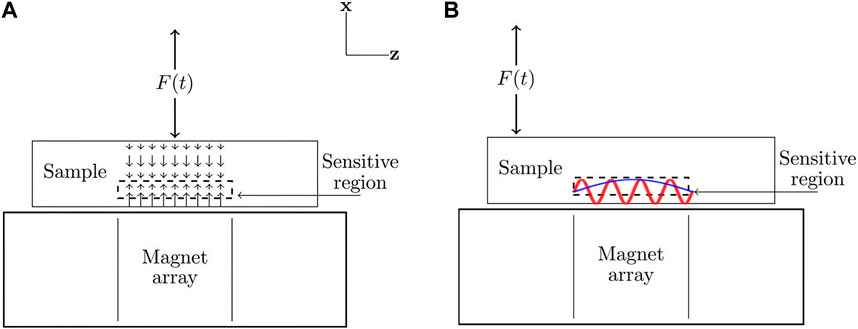
FIGURE 1. Velocity distributions in the sensitive region of a portable magnet array in the presence of longitudinal and shear waves. For longitudinal waves (A), the spatial velocity distribution is uniform and velocity can be measured directly through the phase of the MR signal. For shear waves (B), the spatial velocity distribution (and amount of phase interference) is dependent on the wavelength. Shorter wavelengths (shown in red) lead to a greater modulation of signal magnitude compared to longer wavelengths (shown in blue). When exciting shear waves, the force is offset from the sensitive region so that the longitudinal component is negligible.

2.2.1 Viscoelasticity

Consider a perfectly elastic material, such as a spring. When subjected to a sinusoidally oscillating stress, it responds instantaneously with a sinusoidal strain (completely in phase with the applied stress). By contrast, a completely viscous material, such as a dashpot, dissipates energy when subjected to stress and responds with a strain that is 90° out of phase from the applied stress (as stress is proportional to the strain rate). No physical material is free from viscous losses; therefore, all materials are viscoelastic and can be described by combining viscous and elastic models (dashpots and springs). Viscoelastic materials are commonly described using the complex (or dynamic) modulus, E* [68],

$E^{*}=E^{\prime }+i{E}^{″}=|E|e^{i\delta }(6)$

where the real component (storage modulus), E′, and the imaginary component (loss modulus), E″ represent the elastic and viscous characteristics, respectively. Therefore, when a viscoelastic material is subjected to stress, it responds with a phase difference, or loss-angle, δ, between stress and strain.

2.2.2 Signal analysis for compressive stress

The simplest case to consider in elastometry is a sample under compressive stress where only the longitudinal component of the wave is significant in the sensitive region. Consider a sample excited by a sinusoidal force of amplitude, F₀, and frequency, ω,

$\vec{F}\left(t\right)=-F_0\sin \left(\omega t\right)\widehat{x}(7)$

the sample responds with a sinusoidal displacement of amplitude, A, and phase offset, δ, relative to the applied stress

$\vec{x}\left(t\right)=A\sin \left(\omega t-\delta \right)\widehat{x}(8)$

where δ is the loss-angle defined in Equation 6. This simplest approach for calculating the phase accumulated in the MR signal is to Taylor expand the position,

$x\left(t\right)\approx x_0+v_{0}t+\frac{1}{2}{a}_0{t}^2+\cdots (9)$

the relative phase of the MR signal is then given by,

$\varphi =\gamma \left[x_0\int G\left(t\right)dt+v_0\int G\left(t\right)tdt+a_0\int G\left(t\right)t^{2}dt+\cdots \right](10)$

These integrals are referred to as “moments” of the magnetic field gradient and by varying G(t), one can manipulate the effects of motion on the MR signal [69]. In the case of a constant magnetic field gradient, the phase at the first echo is influenced by the average acceleration and velocity within the sensitive region and is given by,

${\varphi }_1={\varphi }_0+\gamma G{v}_{\mathit{avg}}{\tau }^2+\gamma G{a}_{\mathit{avg}}{\tau }^3(11)$

The phase at the second spin-echo is only influenced by the average acceleration and is given by,

${\varphi }_2={\varphi }_0+2\gamma G{a}_{\mathit{avg}}{\tau }^3(12)$

When applying this approximation to an oscillating sample, it is assumed that velocity (and acceleration) remain constant over the time of acquisition. Stated another way, the echo time must be significantly shorter than the period of oscillation. Complications can arise when working with high frequencies, or low amplitudes when longer echo times are needed to maintain phase sensitivity. Alternatively, if the echo time (twice the time between pulses) is significant compared to the period, then the phase of any Nth echo can be determined by integrating x(t) directly,

${\varphi }_N=\frac{\gamma GA}{\omega }\left[-\cos \left(2N\omega \tau +\delta \right)+{\left(-1\right)}^N\left[\cos \left(\delta \right)+2{\displaystyle \sum _{k=0}^{N-1}}\cos \left(\left(2k+1\right)\omega \tau +\delta \right){\left(-1\right)}^k\right]\right](13)$

Encoding motion in the first spin-echo is trivial and can be done using the first odd echo in a Carr-Purcell-Meiboom-Gill sequence (CPMG) [70] (more details on MR pulse sequences can be found in Section 4.1). The second spin-echo can be used if the stimulated echo resulting from imperfect excitation is cancelled with a phase cycle [71]. Subsequent echoes require a more detailed analysis of coherence pathways and thus, were not considered in the research presented in this review, but are a potential area of focus for future investigation.

Measurements of velocity and acceleration at various points throughout the vibration period can be used to characterize the time-varying response of the sample to applied stress. Viscoelastic properties can then be estimated through comparison with independent measurements of the applied stress.

2.2.3 Signal analysis for shear stress

Analysis of the MR signal can become more complicated if the shear component of a wave is dominant within the sensitive region. In addition to the potential effects of velocities distributed in time (finite echo time considerations), spatial velocity distributions can lead to significant phase interference, especially if the wavelength covers a significant fraction of the sensor size. If not properly accounted for, the presence of shear waves can lead to detrimental effects on the MR signal; however, there is also potential for exploiting this dependence to characterize viscoelastic properties.

If viscous effects are significant, there can be a significant reduction in vibration amplitude within the sensitive volume that must be considered. This can be easily seen by considering a plane wave that propagates in the z-direction in a homogeneous, isotropic, linear viscoelastic medium. Particles are displaced in the x-direction with amplitude, A, and frequency, ω,

$x\left(z,t\right)=A{e}^{-\alpha z}\sin \left(kz\right)\sin \left(\omega t\right)+x_0(14)$

where k is the wave-number and α is the attenuation coefficient.

Both the attenuation and shear wave speed are influenced by the viscoelastic properties (storage and loss moduli) of the material [72]. The attenuation coefficient, α, is given by,

$\alpha \left(\omega \right)=\sqrt{\rho {\omega }^2\frac{\sqrt{E^{\prime 2}+E^{\prime \prime 2}}-E^{\prime }}{2\left(E^{\prime 2}+E^{\prime \prime 2}\right)}}(15)$

And the shear wave speed, c, is given by,

$c\left(\omega \right)=\frac{\omega }{k\left(\omega \right)}=\sqrt{\frac{1}{\rho }\frac{2\left(E^{\prime 2}+E^{\prime \prime 2}\right)}{E^{\prime }+\sqrt{E^{\prime 2}+E^{\prime \prime 2}}}}(16)$

Refocusing pulses used to generate echoes in a CPMG sequence result in effective square-wave modulation of the magnetic field gradient [41, 73]. Thus, the gradient can effectively be “synchronized” with oscillations applying pulses separated by integer multiples of the vibration period to generate an oscillating “apparent gradient” (as seen by spins in the sensitive region). In the case of a sinusoidally varying gradient,

$G\left(t\right)=G_0\sin \left(\omega t+\varphi \right)(17)$

To simplify the analysis, it can be assumed that attenuation is negligible within the sensitive volume. The MR signal phase is then given by integrating over integer multiples of the vibration period,

$\varphi \left(z\right)={\int }_0^{nT}\gamma A{G}_0\cos \left(\omega t+\delta \right)\cos \left(kz-\omega t\right)=\frac{\gamma G_{0}AnT}{2}\sin \left(kz\right)\cos \left(\varphi \right)(18)$

In the case of constant gradient portable MR, refocusing pulses results in an effective gradient in the form of a square wave; hence, the coefficient of $\frac{1}{2}$ is replaced by $\frac{2}{\pi }$ [33].

Given the finite dimensions of the MR sensor, the distribution of velocities resulting from the propagating shear wave leads to phase interference that depends on the ratio between the wavelength and sensor size. As this ratio increases, so does the amount of phase interference, and effects on signal magnitude become more apparent.

Consider a simple approximation, a 1D sensitive region, through which the shear wave propagates in the z-direction, with particle displacements in the direction of the gradient (x). If the sensor size covers a complete wavelength, there exists a closed-form analytical solution for the MR signal [33],

$S={\int }_0^{\lambda }\rho e^{-i2\gamma G_{0}AnT\cos \left(\varphi \right)\sin \left(kz\right)}dz\propto \lambda J_0\left(\frac{2\gamma GAnT\cos \varphi }{\pi }\right)(19)$

where J_n is the Bessel function of the first kind of order n defined as follows,

$J_n\left(z\right)=\frac{1}{2\pi i^n}{\int }_0^{2\pi }{e}^{iz\cos \varphi }{e}^{in\varphi }d\varphi (20)$

The “Bessel-like” behaviour of the signal is expected even in cases where the sensor size is smaller than the wavelength. Although closed-form analytical solutions cannot be obtained, the signal can be expressed as a series solution using the Jacobi-Anger expansion [74].

Depending on the physical situation, the analysis can be modified. In this review, we describe the implementation of this simple case; however, the general analysis forms a basis for extensions to more complex situations such as accounting for the presence of 2D harmonics, prominent viscous effects within the sensitive region, and incomplete coverage of the wavelength.

2.3 Flow

Techniques involving the use of conventional MR methods to characterize the rheological properties of fluids have been extensively developed in the sub-field of Rheo-NMR [13]. These methods are conceptually similar to those employed by MRE wherein phase-contrast MR sequences are used to acquire spatially resolved measurements of phase, which are converted into 2D displacement (or velocity) fields. Theoretical models are then employed to characterize rheological properties. The spatial resolution provided by Rheo-NMR techniques allows for the characterization of complex fluids and flow regimes relevant to applications in fields such as food science [75, 76], biomedicine [77, 78], and pharmaceuticals [79, 80]. Rheo-NMR methods typically employ large, vertical-bore superconducting MR spectrometers outfitted with a flow apparatus, placing constraints on the sample size and limiting their viability in industrial applications.

Low-field permanent magnets have been used in rheological experiments in the past, often in the context of integrating permanent magnet arrays into commercially available rheometers [77, 81] to provide measurements of MR relaxation parameters in conjunction with rheological properties. The experiments described in this review aim to employ portable MR instruments in the direct characterization of rheological properties. In these sections, we will describe the use of theoretical equations for the velocity distributions of non-Newtonian fluids in the development of MR signal equations that use the portable MR sensitive region as an integrator to encode the flow velocity and flow behaviour index of Newtonian and non-Newtonian fluids in different laminar flow geometries such as pipe flow and Couette flow (laminar flow between concentric rotating cylinders).

2.3.1 Basic fluid dynamics

The flow measurements outlined in this review describe fluids using a power-law model; however, alternative models can be used as long as it is possible to describe the velocity distribution analytically. There may also be potential for incorporating non-analytical numerical modelling of the velocity distribution into the MR signal analysis, but this has not yet been attempted. Using the power-law model, the shear stress, σ can be related to the shear rate, $\dot{\gamma }$ as follows [82],

$\sigma =m{\dot{\gamma }}^n(21)$

where n is the flow behaviour index and m is the flow consistency index. If n < 1, the fluid is shear thinning and the apparent viscosity decreases with increasing shear rate, while the opposite occurs for shear thickening fluids (n > 1). Different values of n result in changes to the shape of the velocity distributions and the amount of phase interference. In some cases, such as laminar flow, closed-form analytical solutions for the velocity distribution can be determined and used to predict the behaviour of the MR signal. Figure 2 shows laminar pipe flow (Figure 2A) and circular Couette flow (Figure 2B) geometries that are characterized in the experiments discussed in this review.

FIGURE 2

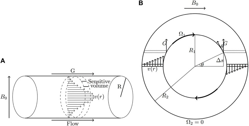
FIGURE 2. Schematics of laminar pipe flow (A) and circular Couette flow (B) (Reprinted from [36], with permission from Elsevier). The shape of the velocity distribution is determined by the flow behaviour index, n. In pipe flow, the entire velocity distribution is aligned with the gradient. In circular Couette flow, opposing velocities on either side of the rotating inner cylinder lead to a net cancellation of phase.

In the case of laminar pipe flow of power-law fluids, the radial distribution of the axial velocity is given by,

$v\left(r\right)=\frac{3n+1}{n+1}{v}_{\mathit{avg}}\left[1-{\left(\frac{r}{R}\right)}^{\frac{1}{n}+1}\right](22)$

where R is the radius of the pipe. In the original work [35], the parameter $n^{\prime }=\frac{1}{n}+1$ was defined for mathematical convenience; however, in most cases in this review, we will use the variable n to describe the flow behaviour index.

For circular Couette flow, more specifically, with a static outer cylinder of radius, R₂, and inner cylinder of radius, R₁ with angular velocity Ω, the radial distribution of the azimuthal velocity component is given by [83],

$v_{\theta }\left(r\right)=r\mathrm{\Omega }\left[\frac{1-{\left(\frac{r}{R_2}\right)}^{-\frac{2}{n}}}{1-{\eta }^{-\frac{2}{n}}}\right](23)$

where r is the radial position inside the pipe and η is the radius ratio, $\frac{R_1}{R_2}$.

Figure 3 shows example velocity profiles for pipe flow (Figure 3A) and circular Couette flow (Figure 3B) of fluids with different values of the flow behaviour index, n, describing a shear-thinning fluid (dashed line), a Newtonian fluid (solid line), and a shear-thickening fluid (dotted line).

FIGURE 3

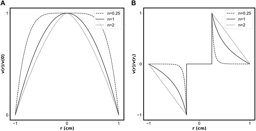
FIGURE 3. Normalized velocity profiles for (A) flow in a pipe of radius 1 cm, and (B) flow between a rotating inner cylinder (R₁ = 0.25 cm) and stationary outer cylinder (R₂ = 1 cm). The dashed line represents a shear-thinning fluid (n = 0.25), the solid line represents a Newtonian fluid (n = 1), and the dotted line represents a shear-thickening fluid (n = 2).

These equations can be used to predict the dependence of MR signal on parameters such as the flow velocity and flow behaviour index, often involving integrals with non-trivial solutions. In the following sections, we will review integration techniques and approximations that have been used to generate analytical solutions and simplify the integration.

2.3.2 Signal analysis for pipe flow

In laminar flow, the velocity distribution is stable and remains constant in time; therefore, the MR signal phase can be approximated using a first-order Taylor approximation,

$\varphi \left(r\right)={\varphi }_0+\gamma Gv\left(r\right){\tau }^2(24)$

Integrating over the dimensions of the pipe, the odd-echo phase can be related to the average velocity as follows,

${\varphi }_{\mathit{odd}}={\varphi }_0+\gamma G{v}_{\mathit{avg}}{\tau }^2(25)$

Thus, the average flow velocity in pipe flow can be determined through measurements of phase at varying echo times while measurement of the average flow velocity directly at a single echo time requires a stationary reference.

Determination of the flow behaviour index, n, requires consideration of the MR signal magnitude. The normalized signal of all odd echoes due to phase accumulation can be expressed as,

$S_{\varphi }=\frac{\iint e^{-i\varphi \left(r\right)}rdrd\theta }{\iint ds}=\frac{\int \cos \varphi \left(r\right)rdr}{\int rdr}-i\frac{\int \sin \varphi \left(r\right)rdr}{\int rdr}(26)$

A thorough analytical treatment of these integrals can be found in [35]. Here, we provide the final solution for the normalized magnitude of odd echoes due to phase accumulation,

$M_{\varphi }=\sqrt{S_{Re}^2+S_{Im}^2}=\frac{2}{n^{\prime }{X}^{\frac{2}{n^{\prime }}}}\sqrt{\left(\mathrm{\Gamma }\left(\frac{2}{n^{\prime }}\right)-\mathrm{\Gamma }\left(\frac{2}{n^{\prime }},Xi\right)\right)\left(\mathrm{\Gamma }\left(\frac{2}{n^{\prime }}\right)-\mathrm{\Gamma }\left(\frac{2}{n^{\prime }},-Xi\right)\right)}(27)$

where $X=\frac{n^{\prime }+2}{n^{\prime }}\gamma G{v}_{\mathit{avg}}{\tau }^2$, $n^{\prime }=\frac{1}{n}+1$, and $\mathrm{\Gamma }(a,x)={\int }_x^{\infty }{w}^{a-1}{e}^{-w}dw$.

Several measurement schemes can be used to extract the flow parameters using Eqs 25, 27.

• Use only the first echo to calculate laminar flow parameters. The v_avg is determined from the echo net-phase accumulation using Eq. 25 and used in Equation 27 to determine n′. Using only one odd echo data point suffers from noise, and is not reliable in realistic flow measurements.

• Fit only the magnitude of first odd echoes at different τ to determine v_avg and n′ directly. Fitting to two parameters in Equation 27 can strongly reduce the fitting accuracy.

• Fit the net phase accumulation of first odd echoes at different τ to Equation 25 to determine v_avg. Then, use the fitted v_avg as a constant in Equation 27 to determine n′.

The equations defined above are valid if the fluid within the sensitive volume is completely polarized. The following equations describing incomplete polarization have been verified on a 4.7 T vertical bore instrument [84], the ultimate goal is to translate this work to a portable MR instrument.

${\varphi }_{\mathit{odd}}^{\prime }=\left\{\begin{array}{cc}\arctan \left(\frac{{}_{0}D_{t=\frac{1}{c}}^{-\frac{2}{n^{\prime }}+1}\left(\left(1-e^{-\frac{1}{t}}\right)\left(\frac{1}{C}-t\right)\sin \left(At\right)\right)}{{}_{0}D_{t=\frac{1}{c}}^{-\frac{2}{n^{\prime }}+1}\left(\left(1-e^{-\frac{1}{t}}\right)\left(\frac{1}{C}-t\right)\cos \left(At\right)\right)}\right),\hfill & 1<n^{\prime }<2,\hfill \\ \arctan \left(\frac{{}_{0}N_{t=\frac{1}{c}}\left(e^{-\frac{1}{t}}\sin \left(At\right)\right)}{{}_{0}N_{t=\frac{1}{c}}\left(e^{-\frac{1}{t}}\cos \left(At\right)\right)}\right),n^{\prime }=2,\hfill \\ \arctan \left(\frac{{}_{0}D_{t=\frac{1}{c}}^{-\frac{2}{n^{\prime }}}\left(\left(1-e^{-\frac{1}{t}}\right)\sin \left(At\right)\right)}{{}_{0}D_{t=\frac{1}{c}}^{-\frac{2}{n^{\prime }}}\left(\left(1-e^{-\frac{1}{t}}\right)\cos \left(At\right)\right)}\right),n^{\prime }>2,\hfill \end{array}\right.(28)$

$M_{\varphi }^{\prime }=\left\{\begin{array}{cc}\mathrm{\Gamma }\left(\frac{2}{n^{\prime }}-1\right)\frac{2C^{\frac{2}{n^{\prime }}}}{n^{\prime }}\sqrt{\left[{}_{0}D_{t=\frac{1}{c}}^{-\frac{2}{n^{\prime }}+1}\left(\left(1-e^{-\frac{1}{t}}\right)\left(\frac{1}{C}-t\right)e^{-iAt}\right)\right]\left[{}_{0}D_{t=\frac{1}{c}}^{-\frac{2}{n^{\prime }}+1}\left(\left(1-e^{-\frac{1}{t}}\right)\left(\frac{1}{C}-t\right)e^{\mathit{iAt}}\right)\right]},\hfill & 1<n^{\prime }<2,\hfill \\ C\sqrt{\left[{}_{0}N_{t=\frac{1}{c}}\left(e^{-\frac{1}{t}}{e}^{-iAt}\right)\right]\left[{}_{0}N_{t=\frac{1}{c}}\left(e^{-\frac{1}{t}}{e}^{\mathit{iAt}}\right)\right]},n^{\prime }=2,\hfill \\ \mathrm{\Gamma }\left(\frac{2}{n^{\prime }}\right)\frac{2C^{\frac{2}{n^{\prime }}}}{n^{\prime }}\sqrt{\left[{}_{0}D_{t=\frac{1}{c}}^{-\frac{2}{n^{\prime }}}\left(\left(1-e^{-\frac{1}{t}}\right)e^{-iAt}\right)\right]\left[{}_{0}D_{t=\frac{1}{c}}^{-\frac{2}{n^{\prime }}}\left(\left(1-e^{-\frac{1}{t}}\right)e^{\mathit{iAt}}\right)\right]},n^{\prime }>2,\hfill \end{array}\right.(29)$

where Γ(x) is the gamma function $\mathrm{\Gamma }(x)={\int }_0^{\infty }{w}^{x-1}{e}^{-w}dw$; ${}_{a}D_x^{-p}f(x)$ is the Riemann-Liouville fractional integral ${}_{a}D_x^{-p}f(x)=\frac{1}{\mathrm{\Gamma }(p)}{\int }_a^x{(x-w)}^{p-1}f(w)dw$; ${}_{a}N_{x}f(x)$ is defined as ${}_{a}N_{x}f(x)={\int }_a^{x}f(w)dw$; $C=\frac{L_{\mathit{pol}}}{T_1{V}_{\max }}=\frac{n^{\prime }{L}_{\mathit{pol}}}{(n^{\prime }+2)T_1{V}_{\mathit{avg}}}$; and $A=\gamma G{v}_{\max }{\tau }^{2}C=\frac{\gamma G{L}_{\mathit{pol}}{\tau }^2}{T_1}$. γ is the gyromagnetic ratio, G the gradient in the flow direction, and 2τ the CPMG echo time.

2.3.3 Signal analysis for Couette flow

For circular Couette flow, the symmetry of the velocity distribution leads to a net cancellation of phase; however, the above approach can be used to extract the flow behaviour index from the signal magnitude. Taking the component of the azimuthal velocity distribution (Eq. 23) in the direction of the magnetic field gradient, the MR signal magnitude is given by,

$S={\int }_{R_1}^{R_2}\rho \left(r\right){\int }_{{\theta }_1}^{{\theta }_2}{e}^{-i\left(\gamma G{v}_{\theta }\left(r\right)\cos \theta {\tau }^2\right)}rdrd\theta (30)$

Assuming the spin density distribution ρ(r), is uniform within the excited slice, ρ(r) = 1.

Given the geometry of the flow system, the magnitude can change significantly depending on the dimensions of the excited slice (a vertical cross-section of the outer cylinder). We present two approximations that can be used to simplify the MR signal analysis depending on the dimensions of the excited slice (only the thin slice approach has been verified experimentally):

• Complete coverage: If the dimensions of the excited slice are comparable to those of the Couette cell. This approximation requires small samples or weak gradients (wide bandwidths of excitation). Sample alignment problems are less likely; however, there is a greater possibility for complications due to B₁ field homogeneity.

• Thin slice excitation: If the dimensions of the excited slice are significantly smaller than the dimensions of the Couette cell. This works in stronger magnetic field gradients; however, sample alignment becomes important and SNR is impacted by the reduced sample volume.

In the complete coverage case, a Bessel function comes from integration over angular coordinate, θ. The remaining integral over the radial coordinate is non-trivial and can be performed numerically.

$S=2\pi {\int }_{R_1}^{R_2}{J}_0\left(\gamma G{v}_{\theta }\left(r\right){\tau }^2\right)rdr(31)$

In the thin-slice approximation, the angular coordinate is fixed, and the integration over the radial coordinate can be performed numerically.

$S={\int }_{R_1}^{R_2}\cos \left(\gamma G{v}_{\theta }\left(r\right)\cos \theta {\tau }^2\right)rdr(32)$

We bring attention to two important consequences of the thin-slice approximation. The first is the need for precise knowledge of the slice position relative to the center of the Couette cell (or the angle between the velocity and magnetic field gradient, θ). Second is the reduction in sample volume and by extension, SNR. Practical considerations that can be used to account for these limitations will be described in Section 4.1.2 on experimental procedures.

3 Instrumentation

One key advantage of portable MR phase interference-based methods is that there are only two core requirements of the instrumentation: a known magnetic field distribution within a well-defined sensitive volume and dominant motion in the direction of the gradient. As a result, designs of magnets and radiofrequency (RF) probes can be modified to fit a given application. In this section, we will establish the accessibility of phase interference-based methods by reviewing two simple magnet array designs (shown in Figure 4) that were used to encode motion in example experiments.

FIGURE 4

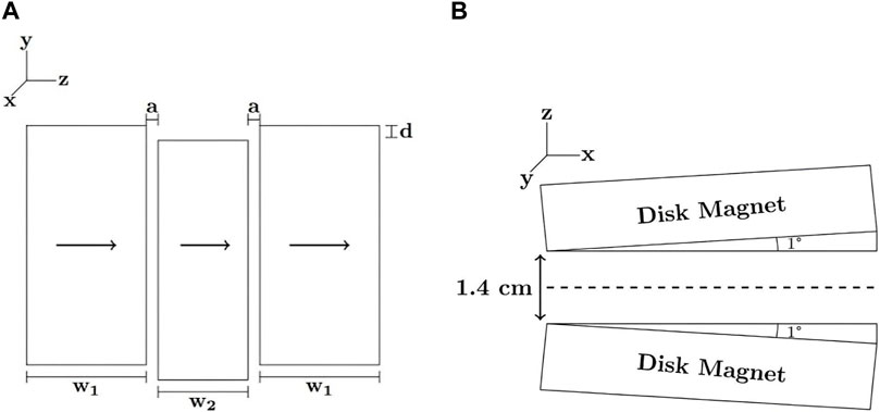
FIGURE 4. Example magnet designs used in constant gradient phase interference-based experiments. The three-magnet array shown in (A) consists of three rectangular permanent magnets, arranged to provide a constant gradient in a finite region (1.5 cm × 1.5 cm) in the y-direction. The Proteus magnet shown in (B) consists of two disk magnets separated by 1 cm and tilted by 1° to achieve a constant gradient of 60 G/cm in the x-direction.

When using conventional MR systems, one might begin with a desired measurement and search for existing MR instruments on which it can be performed. Given the low cost of portable MR sensors, one can afford to take an alternate path. Instead, one might begin with an intended application or experiment, searching for areas that could benefit from the aforementioned advantages of MR. Next, the magnetic field profile and magnet geometry can be estimated based on the associated range of velocities. Finally, simulation methods can be used to optimize the spatial configuration of several permanent magnets in a suitable geometry that achieves the desired distribution. Once an instrument has been constructed and tested, one can attempt to employ it in a range of applications to investigate other potential portable MR techniques.

Although the experiments outlined in the following sections were initially conducted on a limited number of portable MR instruments, there exists an abundance of alternative magnet designs that can effectively employ the phase interference technique. While a relatively large, constant gradient is considered optimal due to its enhanced motion sensitivity and simplified analysis, any portable MR instrument with a known magnetic field distribution (preferably a constant gradient) can be employed. Other portable MR instruments have been specifically engineered to offer homogeneous magnetic fields or constant gradients within well-defined sensitive regions, employing both unilateral [85, 86] and closed-bore geometries [87, 88].

In some cases (such as in shear wave experiments) it was easier to employ a commercially available portable MR sensor. Commercial instruments are typically more stable and robust, have improved sensitivity, and can be used to rapidly demonstrate proof-of-concept. The sensitive volume of the commercial instrument (with a lateral size of 9 × 19 (±1) mm) was displaced 3 mm from the surface of the magnet and contained a mean gradient of 1265 G/cm.

Custom-built instruments such as the three-magnet array employed in longitudinal wave elastometry and Couette flow experiments provide more flexibility, as they can easily be modified for use in different experimental conditions. The magnet array consists of three NdFeB permanent magnets in an optimized spatial configuration to provide a constant magnetic field gradient within a finite sensitive region [25]. The optimal spatial configuration was determined by approximating the magnet blocks as infinite sheets of current and calculating the magnetic field and superimposing the results according to their positions in the y-z plane [89].

The magnet array (shown in Figure 4A) consists of three N48 NdFeB permanent magnets of 10 cm × 5 cm × 3 cm size (external blocks) and 10 cm × 5 cm × 2 cm (central block) placed in an aluminum box separated by 4.76 mm thick fibreglass spacers. The central block was displaced by 2 mm to provide a constant gradient of 254 G/cm in a finite sensitive region (approx. 1.5 cm × 1.5 cm in the y-z plane) that extends from approx. 0.5–3.5 cm above the surface of the magnet.

Careful choice of RF probe designs can provide flexibility in the use of a single magnet design in several different motion-encoding applications. RF probe design can be determined by considering factors such as the geometry of samples, ease of inducing motion in the direction of the gradient, and the dimensions and homogeneity of the excited slice.

Surface coils are ideal for applications involving large samples that are inaccessible to other coil geometries. Because the filling factor of a surface coil is high, its sensitivity is very high when one is interested in a small sample volume [90]. The penetration depth is determined by the diameter of the surface coil, and the sensitive region of a surface coil of radius a is often defined by the region $\frac{a}{2}<y<a$ [90], where y is the distance above the surface coil. For elastometry measurements, a surface coil (approx. 2 cm in diameter) was tuned to a frequency of 5.43 MHz and positioned inside the sensitive spot (approx. 2 cm from the surface of the magnet).

Solenoidal coils are cylindrically shaped and produce a magnetic field parallel to the cylinder axis. Although solenoidal coils offer the highest sensitivity, they do have several limitations. The direction of the magnetic field can lead to sample accessibility problems, and coils can become self-resonant at high frequencies (an additional advantage of the low-frequencies of portable MR instruments) [91]. There are many applications where samples have cylindrical geometry, such as Couette and pipe flow, and fit naturally inside solenoidal coils. The solenoidal coil used in Couette flow experiments consisted of five turns of copper wire wound around a 3D-printed former with a diameter of 1.1 cm and height of 1.5 cm and was tuned to a frequency of 5.73 MHz and suspended 1.5 cm in front of the magnet.

Magnet designs such as the PROTEUS (PROTon Embedded sUbmersible Sensor) magnet [24] (shown in Figure 4B) are a natural choice for pipe flows. The flow PROTEUS magnet consists of two N52 NdFeB disk magnets of 5.1 cm diameter and 1.3 cm thickness [35]. A machined casing (6 × 10 × 4 cm³) was fabricated from Garolite (McMaster-Carr G-10 fibreglass laminate) according to a finite element analysis simulation, optimizing the configuration of the magnets to provide a constant gradient along the axis of the magnet bore, with minimal gradients in orthogonal directions. A gradient strength on the order of 60 G/cm was selected to observe flow rates in the average velocity range of 1–5 cm/s with echo times below 1 ms.

The optimal configuration included an edge separation of 1.4 cm and 1° tilt relative to the symmetry axis. The casing included a 1.2 cm diameter cylindrical bore along the direction of the gradient for positioning the flow tubing. Experimental field plots of the assembled magnet array showed a 6 mm region near the origin with a G_x value of 64 G/cm, confirmed by average velocity measurements of known water flows.

A solenoidal RF probe fits naturally with the magnet and pipe flow geometry and provides a homogeneous B₁ excitation of a cylindrical cross-section of the pipe. A four-turn solenoidal coil (1 cm inner diameter) was formed with 0.8 mm diameter copper wire around a glass pipe and capacitively tuned and matched to 20.48 MHz and 50 Ω, respectively. The interior and exterior of the magnet casing were wrapped with 0.2 mm copper tape to limit external RF interference and suppress the effects of acoustic ringing on the detected signal.

In all experiments, RF probes were connected to a Tomco Technologies 250 W RF amplifier. RF pulse sequences were designed using NTNMR software and executed by a TecMag LapNMR console. While the LapNMR console was convenient for these experiments, portable MR instruments can be transferred to alternate acquisition hardware if the need arises.

4 Experimental procedures

A primary advantage of portable MR phase interference-based techniques is the simplicity of the MR pulse sequences. In fact, each experiment is based on a simple spin-echo sequence. Fundamentally, a single spin-echo carries all of the information needed to encode motion in each experiment; however, in practice, slight modifications are needed depending on the geometries and velocity distributions involved. Some parts of this section can be skipped if the reader is experienced with experimental pulse NMR.

4.1 Modifications to a CPMG echo sequence

The spin-echo is a simple pulse sequence that underpins almost all MR experiments performed in inhomogeneous fields. Spin-echoes are formed by applying refocusing pulses to cancel out the effects of offset frequencies that lead to dispersion of magnetization in the transverse plane [70, 92, 93]. Echo intensities decay exponentially according to properties such as the transverse relaxation time, T₂, and self-diffusion coefficient, D [93]. Therefore, in most cases, echo trains acquired in the presence of motion were normalized by dividing their echo intensities by those of corresponding echoes of a stationary sample.

Several factors can lead to differences between the measured and idealized echo trains. Most prominent are inhomogeneities in the B₀ and B₁ fields, which lead to distributions in flip angles throughout the sensitive volume and the relative contributions from alternative magnetization pathways that grow exponentially with each pulse (while the overall magnetization decreases). Alternative pathways reduce the contribution of the ideal (90°-τ-180°-τ…) pathway responsible for phase encoding and prevent direct motion encoding using subsequent echoes. Some techniques can be used to eliminate unwanted coherence pathways in subsequent echoes; however, current portable MR methods mostly make use of the first echo to encode motion. Figure 5 shows an example CPMG sequence, with numbers (1–4) indicating features associated with each example experiment described in the following sections.

FIGURE 5

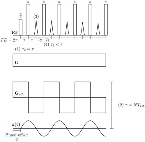
FIGURE 5. All portable MR phase interference-based methods make use of spin echoes in different ways. In detecting longitudinal waves (1) a phase cycle is used to encode velocity information in the first echo and acceleration in the second echo (in this case τ = τ₂). In detecting shear waves (2), the application of RF pulses is synchronized with the external vibrations, giving rise to an effective square wave gradient, encoding information on shear wavelength in signal magnitude. In pipe flow (3) the first odd echo phase and magnitude at variable τ are used to extract rheological properties. In Couette flow (4) the first echo is acquired with variable τ and subsequent echoes are acquired with a short τ₂ and added together to enhance SNR.

4.1.1 Elastometry

Synchronization is a shared feature of both elastometry experiments and can be easily achieved through the use of an external trigger in the acquisition sequence. In the longitudinal case, synchronization of vibrations with the MR acquisition allows for velocity measurements at several points along the vibration period through the introduction of a series of delays before the MR excitation (the effective gradient is constant over the echo acquisition). Measured velocity waveforms can then be compared to obtain relative measurements of viscoelastic properties.

In shear wave experiments, synchronization provides a well-defined square wave modulation of the effective magnetic field gradient with a constant phase offset. It will be shown however, that synchronization is not completely necessary to observe the effects of vibration on the MR signal, and that averaging of random phase offsets still leads to an overall reduction in signal magnitude. Label (2) in Figure 5 indicates synchronization of the CPMG acquisition with the harmonic excitation for τ values that are integer multiples of the vibration period, leading to an effective square wave magnetic field gradient.

Given the sinusoidal motion, another modification allows for the use of the second echo which encodes acceleration. In the general spin echo sequence shown above, the second echo is a superposition of a spin echo (due to the refocusing of the first echo) and a stimulated echo (a result of imperfect RF pulses). The stimulated echo can be cancelled upon even numbers of acquisitions with a slight modification of the CPMG sequence described above where the phase of the first refocusing pulse is cycled between + and − y [71]. Label (1) in Figure 5 indicates the acquisition of the first and second echo with the same τ value.

In compression experiments, the effects of phase interference are minimal, and the motion can be completely characterized by measuring the net-phase accumulation. In shear wave experiments, phase interference depends on the wavelength and phase offset of the propagating shear wave; thus, both magnitude and phase can be used to gain insight into the dynamic properties that influence the shape of the velocity distribution.

4.1.2 Flow

Pipe flow measurements require very few modifications to the general sequence described above. Simply acquiring the spin-echo at a variety of echo times is sufficient to characterize both the average flow velocity (through the phase) and flow behaviour index (through the magnitude). Acceleration is negligible in laminar flow; therefore, the second echo carries no useful information regarding motion. Label (3) in Figure 5 indicates that only the first echo is used in pipe flow measurements,

It is possible to perform Couette flow measurements similarly; however, complications arise due to the small excited volume of the sample, leading to low SNR. These complications are addressed by acquiring a CPMG echo train with a very short echo time following the first motion encoding echo. Given the short echo time, the effect of flow on these echoes is negligible, and they can be added together to enhance SNR [94]. Label (4) in Figure 5 indicates that subsequent echoes are acquired with a shorter echo time.

The other complication that arises when working with thin excited slices in Couette flow is the difficulty in knowing the exact position of the slice across the cylinder. The offset of the excited slice can be measured using another modification to the general spin-echo sequence. Rather than applying a single “hard” 90° excitation pulse, which generates magnetization within a single continuous volume. Several pulses, separated by delays of length, δ, can be applied to generate magnetization within multiple regions of the sample, separated by [95, 96] a distance, $\mathrm{\Delta }x=\frac{2\pi }{\gamma G\delta }$. The offset can be deduced by comparing intensities from each of the excited slices in the 1D profile generated by the Fourier transform of the spin echo.

4.2 Inducing motion

4.2.1 Elastometry

In shear and longitudinal wave experiments, a dual-channel signal generator was used to synchronize the MR acquisition with mechanical vibrations [33, 34]. The first channel sent a signal to a mechanical actuator. Shear waves were transmitted into the samples by an aluminum plate which covered the surface of the sample. Excitation stingers were used to induce longitudinal waves. An excitation stinger is a thin rod that is stiff in the axial direction, and flexible in other directions, ensuring that forces are only transmitted along the axis of the sample.

Both experiments relied on independent measurements of vibration amplitudes displayed on an oscilloscope. In shear wave measurements, an optical sensor was used to scan the sample surface. These measured amplitudes were then used to predict the decay of signal magnitude due to vibrations. In longitudinal wave measurements, a piezoelectric force sensor was positioned between the sample and the excitation stinger. These measurements were compared to the velocity waveforms measured with the portable MR sensor.

4.2.2 Flow

Pipe flow experiments were performed using the gravity-fed flow from a reservoir suspended several feet above the MR sensor and refreshed by fluid pumped from a second reservoir at floor level [35]. A submersible pump was used to ensure a constant pressure head driving the flow, providing more inflow to the upper reservoir than was flowing through the magnet. An overflow in the upper reservoir was used to return excess fluid to the lower reservoir. A flow meter was used to control the average flow rate. Most tubing in the flow network was clear PVC tubing with an inner diameter of 0.8 cm, except for a 70 cm section of 0.67 cm diameter glass tubing that was connected at a distance (of at least 50 diameters) from the opening of the magnet to allow for a steady flow profile to develop. Flow rates were independently measured from outflow using a measuring cylinder and timer.

Couette flow experiments were performed by suspending a 12 V DC motor, attached to a 6 mm diameter inner cylinder inside of a 10 mm sample tube. Rotary seals were fitted into the opening of the sample tube to maintain the central alignment of the inner cylinder [36]. An optical sensor was directed at the rotating inner cylinder to provide independent measurements of the rotation speed, which could be used to calculate the shear rate at the inner wall.

5 Validation and discussion

5.1 Validation

Thus far, we have shown how fundamental theoretical concepts can be used to extend the phase interference idea to several different applications. We have also shown that accessible portable magnet designs can be easily adapted to fit these situations and that motion can be characterized with simple modifications to a general CPMG sequence. In this section, we will present sample results from each of the example experiments, showing how they can be employed to gain insight into the dynamic properties of samples.

5.1.1 Compression elastometry

In compression measurements [34], viscoelastic urethane polymers (Sorbothane) were analyzed due to their long-term stability and well-characterized dynamic properties. The samples varied in hardness and were rated on a durometer scale, with OO40 being the softest, and OO70 the hardest. Dynamic properties were calculated using vibration calculators provided by the manufacturer. Cylindrical samples were cut into 1.65 cm diameter cylinders from 1.27 cm thick rectangular sheets and pre-compressed by approx. 0.15 mm against the surface of the magnet array. Vibrations were induced at 100 Hz along the axis of the sample with forces ranging from 0.7 to 2.1 N peak-to-peak. The MR acquisition was synchronized with vibrations using the external trigger. Echoes were acquired with an echo time (TE = 2τ₁) of 0.5 ms at 10 points along the vibration period (10 ms) by including a table of delays evenly spaced by 1 ms.

Phase in the MR signal was used to determine the velocity, which was plotted alongside the piezoelectric force sensor measurements, allowing for relative comparisons between samples. Velocity waveforms are shown in Figure 6. Symbols represent measured velocities, solid lines represent sinusoidal fits, and dashed lines represent piezoelectric force sensor measurements (shifted in phase by 90° for comparison with velocity waveforms). The differences in viscoelasticity between samples can be seen through the variation in phase offsets and amplitudes. The loss angle was determined through the fitted value of the phase offset and the magnitude of the complex modulus was determined by plotting the MR-measured velocities against force and taking the slope. Figure 7 shows the MR-measured velocities (symbols) plotted against the piezoelectric force sensor measurements for each sample fitted linearly to extract the magnitude of the complex modulus.

FIGURE 6

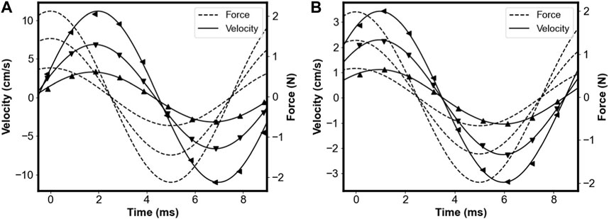
FIGURE 6. Measured velocity waveforms plotted for (A) OO40 and (B) OO70 Sorbothane samples vibrating at 100 Hz. Superimposed using dashed lines are force waveforms measured with the force sensor, shifted in phase by 90°. Reprinted from [34], with permission from Elsevier.

FIGURE 7

FIGURE 7. Velocity plotted against force fitted to a linear model for OO40, OO50, OO60, and OO70 Sorbothane samples. Reprinted from [34], with permission from Elsevier.

Despite clear differences in the responses that depend on the dynamic properties of each sample, an agreement between measured and tabulated values was not achieved. Measured magnitudes of the complex modulus were in closer agreement than loss-angles; however, they were still found to deviate more for softer samples.

Several factors, unrelated to the MR instrumentation, may have contributed to deviations from tabulated properties. Imperfect sample geometries may have resulted in undetected shear components in directions orthogonal to the gradient, delays that were not accounted for may have contributed to additional phase offsets, and positioning of the sensitive slice near the loaded edge of the sample (where strain is larger) may have corresponded to a physical situation not reflected by the geometric parameter.

Although the experiment was not successful in achieving absolute measurement of viscoelastic properties, the relative measurements provide evidence that a portable MR instrument can indeed be used to characterize the viscoelastic properties of samples under longitudinal excitation. Phase measurements using the second echo were also found to be in close agreement with expectations.

5.1.2 Shear wave elastometry

Cylindrical (16 mm thick, 76 mm diameter) polyurethane and square (50 mm × 50 mm × 6 mm) Sorbothane samples were analyzed in shear wave experiments [33]. CPMG echo trains with 16 echoes were acquired with echo times corresponding to half the periods of mechanical vibrations at amplitudes of 0.152, 0.38, 0.48, 0.71, 0.86, 1.01, 1.2, and 1.35 μm.

Figure 8 shows echo intensities (cross symbols) plotted against vibration amplitude for square and cylindrical samples using the first echo (Figures 8A, C) and the second echo (Figures 8B, D). The dash-dotted line shows theoretical predictions obtained using Eq. 19, assuming a constant gradient throughout the sensitive volume. The solid line shows simulations based on the measured gradient distribution throughout the sensitive volume.

FIGURE 8

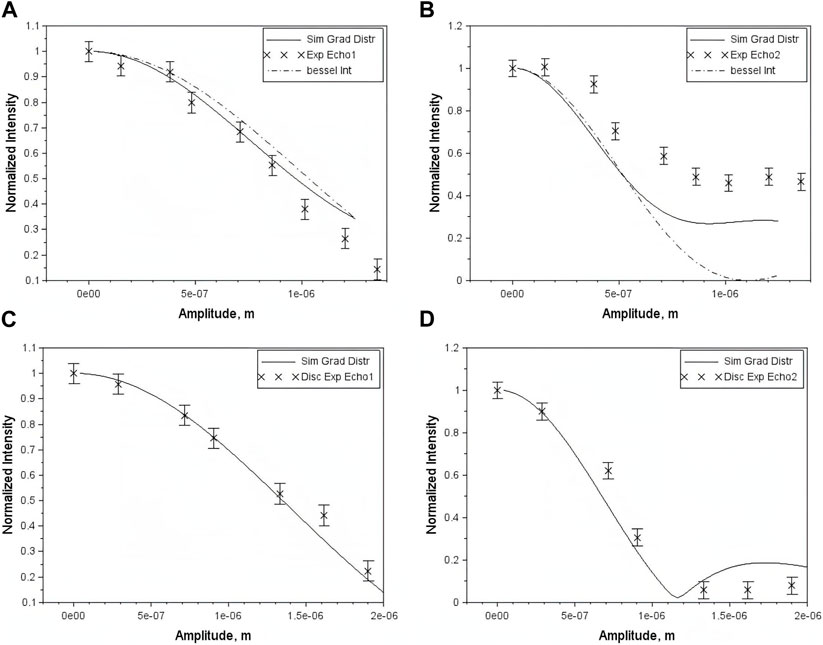
FIGURE 8. The normalized echo intensities vs. the vibration amplitude: experimental data (x), simulations using gradient distribution (solid line) and Bessel integral (-.-). (A)—first echo rectangular sample; (B)—second echo rectangular sample; (C)—first echo cylindrical sample; (D)—second echo cylindrical sample. Reprinted from [33], with permission from Elsevier.

For both samples, the “Bessel Integral” and simulations provide a reasonable fit to the first echo measurements; however, the quality of the fit deteriorates for the second echo, especially at larger amplitudes. Agreement with simulations was improved by accounting for a constant offset associated with incomplete refocusing.

One would expect that the agreement with theory could be further improved by employing the phase cycle described in [71]. Furthermore, the theoretical description assumes that the size of the sensitive volume is comparable to the wavelength. Deviations from this condition result in changes to the velocity distribution present within the sensitive volume, and by extension decreased phase interference and modulation of signal magnitude.

These results demonstrate that, in the presence of strong magnetic field gradients, any active vibration can completely eliminate the MR signal. Therefore, unless the vibration is of interest in the measurement, echo times should be carefully considered for significant attenuation.

A natural approach to decrease vibration effects is to eliminate synchronization; however, we can see that when CPMG measurements are performed at a range of echo times (0.4–1.5 ms, corresponding to frequencies from 1,250 Hz down to 333 Hz) without synchronizing to the vibration of frequency (500 Hz) and amplitude of (255 ± 40 nm), the signal intensity remains sensitive. Figure 9 shows normalized second and third echo intensities, with the most significant signal loss at echo times of 0.9 and 1 ms (when 1/2 TE = 500 Hz).

FIGURE 9

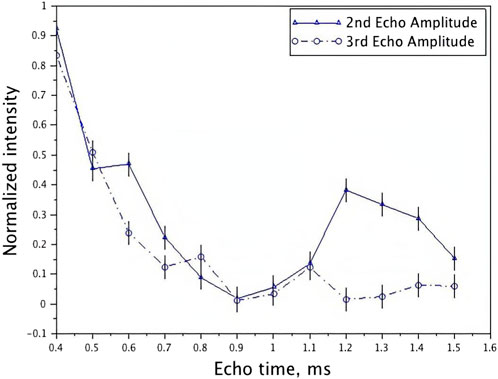
FIGURE 9. Acquisition with no synchronization: second and third echo response to 500 Hz, 0.25 μm vibrations. Echo range is from 0.4 to 1.5 ms. The maximum signal loss occurs when TE = 1 ms as 1/2 TE = 500 Hz. Note the broad spectral response. Note that the echo time, TE = 2τ, with τ defined in Figure 5. Reprinted from [33], with permission from Elsevier.

This type of measurement can be used in two completely different ways. In applications where vibrations are detrimental to the desired measurement, it can be used to characterize the frequency and amplitude of vibrations and select echo times that avoid significant attenuation of signal intensity. There are also clear applications in elastometry, where vibrations can be controlled, allowing measurement of a sample’s viscoelastic properties through the modulation of the signal.

5.1.3 Pipe flow

Two solutions, one Newtonian fluid and one shear-thinning fluid were analyzed in pipe flow experiments [35]. The Newtonian fluid was made by mixing distilled water and glycerol in a ratio of 6:1. For the shear-thinning fluid, xanthan gum was dissolved in distilled water at a concentration of 0.42 wt%. To ensure complete polarization, distilled water and xanthan gum solutions were doped with 0.33 wt% copper sulfate to reduce T₁ lifetimes to 42 and 39 ms, respectively.

Each fluid was measured at two different flow rates. Newtonian fluid experiments were performed at flow rates of 40 ± 1 and 78 ± 1 mL/min corresponding to Reynolds numbers of 82 and 160 (well within the laminar regime typically observed for Reynolds numbers up to 2000). Shear-thinning flow experiments were performed at flow rates of 35 ± 1 and 66 ± 1 mL/min.

Figure 10 shows measurements of the first echo phase at different τ values (dots), fitted using a linear fitting method (shown by solid lines). Close agreement between the fitted and measured average velocities (within 3%) points towards the reliability of the phase-based method for determining the average velocity of laminar flow.

FIGURE 10

FIGURE 10. Processed results of the phase-based method for glycerol/distilled water flows at v_avg = 1.89 ± 0.05 cm/s (A) and for the xanthan gum solution flows at v_avg = 1.65 ± 0.05 cm/s (B). Red dots show the calculated phase accumulation data of the first echo, and the solid line shows the fitted results based on Eq. 25. The fitted ϕ₀ = −0.65 ± 0.01 rad and v_avg = 1.88 ± 0.02 cm/s for (A) and ϕ₀ = −0.58 ± 0.01 rad and v_avg = 1.62 ± 0.02 cm/s for (B). See Figure 5 for a definition of τ. Reprinted from [35] with the permission of AIP Publishing.

Figure 11 shows the normalized magnitude of the first echo. Using the fitted values of v_avg, Eq. 27 was used to fit the data and determine the flow behaviour index.

FIGURE 11

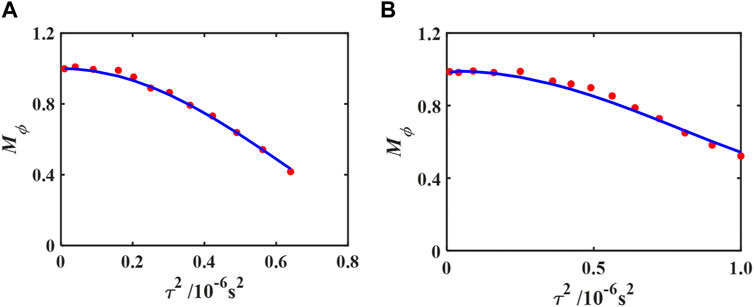
FIGURE 11. Processed results of the magnitude-based method for the glycerol/distilled water flows at v_avg = 1.89 ± 0.05 cm/s (A) and for the xanthan gum solution flows at v_avg = 1.65 ± 0.05 cm/s (B). Red dots show the M_ϕ data of the first echo, and the solid line shows the fitted results based on Eq. 27. The fitted n′ = 2.11 ± 0.06 for (A) and n′ = 5.38 ± 0.19 for (B). See Figure 5 for a definition of τ. Reprinted from [35], with the permission of AIP Publishing.

These results show that measurements of the first odd echo in a CPMG sequence acquired using a portable, low-field MR sensor with a flow-oriented gradient can be directly used for the determination of flow velocity profiles of non-Newtonian fluids.

5.1.4 Couette flow

Four different fluids were analyzed in Couette flow measurements [36]. For a Newtonian fluid, distilled water was doped with copper sulfate at a concentration of 30 mM. A Newtonian oil sample (corn oil) was used to investigate the limitations of diffusive attenuation on the measurement due to its smaller diffusion coefficient. For shear-thinning fluids, xanthan gum was mixed with distilled water in concentrations of 0.2 wt% and 0.4 wt%, and doped with copper sulfate at a concentration of 30 mM.

Calibration was compared using the DANTE and reference sample procedures (described in Section 4.1.2). The offset of the excited slice from the centre of the Couette cell was estimated to be approx. 2.69 mm using the DANTE procedure, and 2.68 mm using distilled water as a reference sample.

Figure 12A shows measurements of signal magnitude (after adding 16 echoes) at a shear rate of 4.85 s⁻¹ normalized to the stationary sample signal at different values of τ₁. There is a clear dependence of signal magnitude on the flow behaviour index, with the distilled water sample (solid line) exhibiting a more rapid decay compared to the 0.2% xanthan gum fluid (dash-dot line) and 0.4% xanthan gum fluid (dashed line). To extract the flow behaviour index, the data were fitted to a numerical integration of Eq. 32. Portable MR-measured flow indices were in close agreement with conventional high-field Rheo-MR measurements on samples with identical xanthan gum concentrations [97].

FIGURE 12

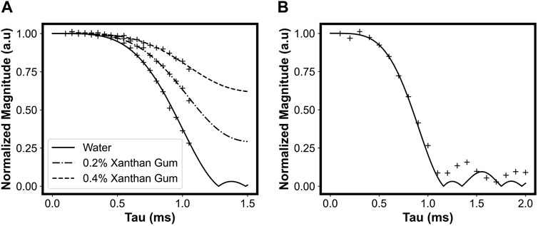
FIGURE 12. (A) Measurements of normalized magnitude (after adding echoes) vs. τ₁ at a shear rate of 4.85 s⁻¹. Symbols represent measured data. Predicted behaviour is shown for water (solid line), 0.2% wt. xanthan gum (dash-dot line), and 0.4% wt. xanthan gum (dashed line). (B) Measurements of normalized magnitude vs. τ₁ at a shear rate of 4.85 s⁻¹ for a sample of corn oil. See Figure 5 for a definition of τ. Reprinted from [36], with permission from Elsevier.

Figure 12B investigates the effects of Couette flow on signal magnitude at longer echo times, taking advantage of the smaller diffusion coefficient of the corn oil sample. Again, measurements agree with theoretical predictions initially, and while oscillations in signal magnitude are observed after τ₁ = 1 ms, they do not occur with the expected amplitude or frequency.

These results further validate the methods used to characterize laminar pipe flows of non-Newtonian fluids and provide a basis for future research on other rotating flows.

6 Conclusion

In this review, we have described the three major facets of portable MR phase interference-based techniques from several different experimental perspectives. We followed the development of several example experiments, describing the fundamental theoretical concepts, instrumentation, experimental procedures, and example results. Each section attempted to emphasize a key advantage of portable MR techniques.

Beginning with the general background and theory, we emphasized the versatility of phase-interference-based methods by describing how a fundamentally simple analysis of MR signal could be extended to predict the response to the motion under several different conditions. This covered cases; with minimal phase interference (longitudinal elastometry) where phase measurements of different points along the vibration period can be used to calculate velocity waveforms and extract relative measurements of viscoelasticity; partial phase interference (pipe flow) where measurements of signal magnitude and phase could be used to extract parameters such as the flow behaviour index and average flow velocity in non-Newtonian fluids; complete phase interference (Couette flow) where solely the signal magnitude can be used to measure the flow behaviour index; and, variable phase interference (shear wave elastometry) where the amount of phase interference and modulation of signal magnitude depends on the wavelength of the shear wave in the sensitive region.

In the subsequent sections on instrumentation and experimental procedures, we emphasized the accessibility of phase interference-based methods by describing how with careful consideration, a single portable magnet array can be employed in vastly different applications. We also showed how one of the most fundamental pulse sequences in MR (the spin echo) allows for motion encoding in each of the example experiments, requiring only slight modifications.

Experimental results, in addition to serving as validation for each experiment, contribute to the broader narrative on the potential and overall validity of portable MR methods. By showing that portable MR methods can be used to quantitatively characterize dynamic properties (in either a relative or direct sense), we can see a clear potential for the development of novel techniques that allow for new and exciting applications of magnetic resonance.

Future work can focus on identifying specific features unique to each experiment, as well as more general features shared by multiple experiments. Analysis methods could be expanded to describe motion in different scenarios, such as complete coverage in Couette flow or pipe flow with incomplete polarization, incomplete coverage of the wavelength in shear wave elastometry, or multifrequency excitation in elastometry. Additionally, new acquisition procedures could be developed, such as investigating the use of additional even and odd CPMG echoes to reduce the overall experiment time.

Core principles such as choosing simplicity over complexity, and designing instrumentation around specific targeted applications are shared by all experiments discussed in this review. This philosophy, if applied correctly, has the potential of introducing powerful magnetic resonance techniques to novel industrial and biomedical applications.

Portable MR methods do have their own limitations and are unable to compete with conventional MRI scanners in an SNR comparison; however, SNR is irrelevant if the sample is inaccessible, or if the acquisition procedures are too complex for real-world applications. We believe that myriad applications may benefit from the implementation of simple, accessible, targeted techniques that provide the fundamental advantages of magnetic resonance in characterizing a well-defined parameter of interest.

Any material that contains MR-sensitive nuclei has a lifetime greater than 1 ms, and responds to stress with a known theoretical velocity distribution is an ideal candidate for portable MR, phase-interference-based methods. In fluid rheology, emulsions systems such as those commonly found in foods, pharmaceuticals, and cosmetics, have been analyzed by conventional Rheo-NMR methods in the past [80] and are candidates for portable NMR analysis. In elastometry, tissues within 1 cm of the surface of the skin such as the epidermis, dermis, and subcutaneous tissue are all MR-sensitive and are realistic candidates for a portable MR measurement. Industrial materials such as SBR vulcanizates have also been analyzed by MR [98] in the past and are candidates for portable MR phase-interference methods.

While the end product is an accessible and robust measurement technique, the design process can be far from simple. Designing experiments around specific applications often brings forth specific problems that must be solved. In many cases, employing an existing technique is significantly easier than starting from scratch with a portable MR instrument. However, each problem that is solved in the continued development of portable MR techniques will make the development of future targeted techniques more efficient. Certainly, there will be cases where portable MR techniques fail to compete with existing methods. The specific applications illustrated here are less important than the fact that they serve as examples of the potential of portable MR. In each case, important information has been gained through the development process, information that is now being applied to expand the range of possible applications of magnetic resonance methods.

Author contributions

WS wrote the manuscript. BB, BN, and IM provided revisions to the draft manuscript. All authors contributed to the article and approved the submitted version.

Funding

WS thanks the New Brunswick Innovation Foundation (NBIF) for funding received under a Graduate Merit Scholarship. BB thanks NSERC of Canada for a Discovery Grant (No. 2022-04003). BN thanks NSERC of Canada for a Discovery Grant (No. 2017-04564). IM thanks the NBIF for a Research Assistantship Grant and NSERC of Canada for a Discovery Grant (No. 2018-04041).

Acknowledgments

The authors gratefully acknowledge the effort undertaken by the individual authors of the various research papers outlined in detail in this review. We also extend our appreciation to Elsevier and AIP Publishing for granting republishing rights for many of the figures included in this manuscript.

Conflict of interest

The authors declare that the research was conducted in the absence of any commercial or financial relationships that could be construed as a potential conflict of interest.

Publisher’s note

All claims expressed in this article are solely those of the authors and do not necessarily represent those of their affiliated organizations, or those of the publisher, the editors and the reviewers. Any product that may be evaluated in this article, or claim that may be made by its manufacturer, is not guaranteed or endorsed by the publisher.

References

1. Lauterbur PC. Image formation by induced local interactions: Examples employing nuclear magnetic resonance. Nature (1973) 242:190–1. doi:10.1038/242190a0

CrossRef Full Text | Google Scholar

2. Tanner JE. Use of the stimulated echo in NMR diffusion studies. J Chem Phys (1970) 52:2523–6. doi:10.1063/1.1673336

CrossRef Full Text | Google Scholar

3. Grover T, Singer JR. NMR spin-echo flow measurements. J Appl Phys (1971) 42:938–40. doi:10.1063/1.1660189

CrossRef Full Text | Google Scholar

4. Hayward R, Packer K, Tomlinson D. Pulsed field-gradient spin echo N.M.R studies of flow in fluids. Mol Phys (1972) 23:1083–102. doi:10.1080/00268977200101061

CrossRef Full Text | Google Scholar

5. Galvosas P, Callaghan PT. Fast magnetic resonance imaging and velocimetry for liquids under high flow rates. J Magn Reson (2006) 181:119–25. doi:10.1016/j.jmr.2006.03.020

PubMed Abstract | CrossRef Full Text | Google Scholar

6. Ahola S, Perlo J, Casanova F, Stapf S, Blümich B. Multiecho sequence for velocity imaging in inhomogeneous rf fields. J Magn Reson (2006) 182:143–51. doi:10.1016/j.jmr.2006.06.017

PubMed Abstract | CrossRef Full Text | Google Scholar

7. Sederman AJ, Mantle MD, Buckley C, Gladden LF. MRI technique for measurement of velocity vectors, acceleration, and autocorrelation functions in turbulent flow. J Magn Reson (2004) 166:182–9. doi:10.1016/j.jmr.2003.10.016

PubMed Abstract | CrossRef Full Text | Google Scholar

8. Muthupillai R, Lomas DJ, Rossman PJ, Greenleaf JF, Manduca A, Ehman RL. Magnetic resonance elastography by direct visualization of propagating acoustic strain waves. Science (1995) 269:1854–7. doi:10.1126/science.7569924

PubMed Abstract | CrossRef Full Text | Google Scholar

9. Venkatesh SK, Yin M, Ehman RL. Magnetic resonance elastography of liver: Technique, analysis, and clinical applications. J Magn Reson Imaging (2013) 37:544–55. doi:10.1002/jmri.23731

PubMed Abstract | CrossRef Full Text | Google Scholar

10. Pepin KM, Ehman RL, McGee KP. Magnetic resonance elastography (mre) in cancer: Technique, analysis, and applications. Prog Nucl Magn Reson Spectrosc (2015) 90-91:32–48. doi:10.1016/j.pnmrs.2015.06.001

PubMed Abstract | CrossRef Full Text | Google Scholar

11. Venkatesh SK, Ehman RL. Magnetic resonance elastography of abdomen. Abdom Imaging (2014) 40:745–59. doi:10.1007/s00261-014-0315-6

CrossRef Full Text | Google Scholar

12. Ringleb SI, Bensamoun SF, Chen Q, Manduca A, An KN, Ehman RL. Applications of magnetic resonance elastography to healthy and pathologic skeletal muscle. J Magn Reson Imaging (2007) 25:301–9. doi:10.1002/jmri.20817

PubMed Abstract | CrossRef Full Text | Google Scholar

13. Coussot P. Progress in rheology and hydrodynamics allowed by NMR or MRI techniques. Experiments in Fluids (2020) 61:207. doi:10.1007/s00348-020-03037-y

CrossRef Full Text | Google Scholar

14. Callaghan PT. Rheo-NMR: A new window on the rheology of complex fluids. New Jersey: John Wiley & Sons, Ltd (2012). doi:10.1002/9780470034590.emrstm0470.pub2

CrossRef Full Text | Google Scholar

15. Callaghan PT. Rheo NMR and shear banding. Rheologica Acta (2008) 47:243–55. doi:10.1007/s00397-007-0251-2

CrossRef Full Text | Google Scholar

16. Al-kaby RN, Codd SL, Seymour JD, Brown JR. Characterization of velocity fluctuations and the transition from transient to steady state shear banding with and without pre-shear in a wormlike micelle solution under shear startup by Rheo-NMR. Appl Rheology (2020) 30:1–13. doi:10.1515/arh-2020-0001

CrossRef Full Text | Google Scholar

17. Seymour JD, Manz B, Callaghan PT. Pulsed gradient spin echo nuclear magnetic resonance measurements of hydrodynamic instabilities with coherent structure: Taylor vortices. Phys Fluids (1999) 11:1104–13. doi:10.1063/1.869981

CrossRef Full Text | Google Scholar

18. Blümich B, Blümler P, Eidmann G, Guthausen A, Haken R, Schmitz U, et al. The NMR-mouse: Construction, excitation, and applications. Magn Reson Imaging (1998) 16:479–84. doi:10.1016/s0730-725x(98)00069-1

PubMed Abstract | CrossRef Full Text | Google Scholar

19. Casanova F, Perlo J, Blümich B. Single-sided NMR. Berlin Heidelberg: Springer (2011). doi:10.1007/978-3-642-16307-4

CrossRef Full Text | Google Scholar

20. Utsuzawa S, Fukushima E. Unilateral NMR with a barrel magnet. J Magn Reson (2017) 282:104–13. doi:10.1016/j.jmr.2017.07.006

PubMed Abstract | CrossRef Full Text | Google Scholar

21. Paetzold RF, Matzkanin GA, Santos ADL. Surface soil water content measurement using pulsed nuclear magnetic resonance techniques. Soil Sci Soc America J (1985) 49:537–40. doi:10.2136/sssaj1985.03615995004900030001x

CrossRef Full Text | Google Scholar

22. Glover P, Aptaker P, Bowler J, Ciampi E, McDonald P. A novel high-gradient permanent magnet for the profiling of planar films and coatings. J Magn Reson (1999) 139:90–7. doi:10.1006/jmre.1999.1772

PubMed Abstract | CrossRef Full Text | Google Scholar

23. McDonald P, Aptaker P, Mitchell J, Mulheron M. A unilateral NMR magnet for sub-structure analysis in the built environment: The surface GARField. J Magn Reson (2007) 185:1–11. doi:10.1016/j.jmr.2006.11.001

PubMed Abstract | CrossRef Full Text | Google Scholar

24. Ross MM, Wilbur GR, Barrita PFJC, Balcom BJ. A portable, submersible, MR sensor – The Proteus magnet. J Magn Reson (2021) 326:106964. doi:10.1016/j.jmr.2021.106964

PubMed Abstract | CrossRef Full Text | Google Scholar

25. García-Naranjo JC, Mastikhin IV, Colpitts BG, Balcom BJ. A unilateral magnet with an extended constant magnetic field gradient. J Magn Reson (2010) 207:337–44. doi:10.1016/j.jmr.2010.09.018

PubMed Abstract | CrossRef Full Text | Google Scholar

26. Marble AE, Mastikhin IV, Colpitts BG, Balcom BJ. A constant gradient unilateral magnet for near-surface MRI profiling. J Magn Reson (2006) 183:228–34. doi:10.1016/j.jmr.2006.08.013

PubMed Abstract | CrossRef Full Text | Google Scholar

27. Richard SJ, Newling B. Measuring flow using a permanent magnet with a large constant gradient. Appl Magn Reson (2019) 50:627–35. doi:10.1007/s00723-018-1107-x

CrossRef Full Text | Google Scholar

28. Osán T, Ollé J, Carpinella M, Cerioni L, Pusiol D, Appel M, et al. Fast measurements of average flow velocity by low-field 1H NMR. J Magn Reson (2011) 209:116–22. doi:10.1016/j.jmr.2010.07.011

PubMed Abstract | CrossRef Full Text | Google Scholar

29. Fridjonsson EO, Stanwix PL, Johns ML. Earth’s field nmr flow meter: Preliminary quantitative measurements. J Magn Reson (2014) 245:110–5. doi:10.1016/j.jmr.2014.06.004

PubMed Abstract | CrossRef Full Text | Google Scholar

30. Benson T, Mcdonald P. Profile amplitude modulation in stray-field magnetic-resonance imaging. J Magn Reson Ser A (1995) 112:17–23. doi:10.1006/jmra.1995.1004

CrossRef Full Text | Google Scholar

31. Song YQ, Scheven UM. An NMR technique for rapid measurement of flow. J Magn Reson (2005) 172:31–5. doi:10.1016/j.jmr.2004.09.018

PubMed Abstract | CrossRef Full Text | Google Scholar

32. Silva PF, Jouzdani MA, Condesso M, Hurtado Rivera AC, Jouda M, Korvink JG. Net-phase flow NMR for compact applications. J Magn Reson (2022) 341:107233. doi:10.1016/j.jmr.2022.107233

PubMed Abstract | CrossRef Full Text | Google Scholar

33. Mastikhin I, Barnhill M. Sensitization of a stray-field NMR to vibrations: A potential for MR elastometry with a portable NMR sensor. J Magn Reson (2014) 248:1–7. doi:10.1016/j.jmr.2014.09.003

PubMed Abstract | CrossRef Full Text | Google Scholar

34. Selby W, Garland P, Mastikhin I. Dynamic mechanical analysis with portable NMR. J Magn Reson (2022) 339:107211. doi:10.1016/j.jmr.2022.107211

PubMed Abstract | CrossRef Full Text | Google Scholar

35. Guo J, Ross MMB, Newling B, Lawrence M, Balcom BJ. Laminar flow characterization using low-field magnetic resonance techniques. Phys Fluids (2021) 33:103609. doi:10.1063/5.0065986

CrossRef Full Text | Google Scholar

36. Selby W, Garland P, Mastikhin I. A simple portable magnetic resonance technique for characterizing circular Couette flow of non-Newtonian fluids. J Magn Reson (2022) 345:107325. doi:10.1016/j.jmr.2022.107325

PubMed Abstract | CrossRef Full Text | Google Scholar

37. Kuethe DO, Herfkens RJ. Fluid shear and spin-echo images. Magn Reson Med (1989) 10:57–70. doi:10.1002/mrm.1910100106

PubMed Abstract | CrossRef Full Text | Google Scholar

38. Bãlibanu F, Hailu K, Eymael R, Demco D, Blümich B. Nuclear magnetic resonance in inhomogeneous magnetic fields. J Magn Reson (2000) 145:246–58. doi:10.1006/jmre.2000.2089

PubMed Abstract | CrossRef Full Text | Google Scholar

39. Nishimura DG. Principles of magnetic resonance imaging. Stanford, California: Selfpublished (2010).

Google Scholar

40. Fukushima E, Roeder SB. Experimental pulse NMR. United States: CRC Press (2018). doi:10.1201/9780429493867

CrossRef Full Text | Google Scholar

41. Stepišnik J. Analysis of NMR self-diffusion measurements by a density matrix calculation. Physica B+C (1981) 104:350–64. doi:10.1016/0378-4363(81)90182-0

CrossRef Full Text | Google Scholar

42. Hirsch S, Braun J, Sack I. Magnetic resonance elastography: Physical background and medical applications. United States: Wiley (2017).

Google Scholar

43. Uffmann K, Ladd M. Actuation systems for MR elastography. IEEE Eng Med Biol Mag (2008) 27:28–34. doi:10.1109/emb.2007.910268

PubMed Abstract | CrossRef Full Text | Google Scholar

44. Doyley MM. Model-based elastography: A survey of approaches to the inverse elasticity problem. Phys Med Biol (2012) 57:R35–R73. doi:10.1088/0031-9155/57/3/r35

PubMed Abstract | CrossRef Full Text | Google Scholar

45. Fovargue D, Nordsletten D, Sinkus R. Stiffness reconstruction methods for MR elastography. NMR Biomed (2018) 31:e3935. doi:10.1002/nbm.3935

PubMed Abstract | CrossRef Full Text | Google Scholar

46. Oliphant TE, Manduca A, Ehman RL, Greenleaf JF. Complex-valued stiffness reconstruction for magnetic resonance elastography by algebraic inversion of the differential equation. Magn Reson Med (2001) 45:299–310. doi:10.1002/1522-2594(200102)45:2⟨299::aid-mrm1039⟩3.0.co;2-o

PubMed Abstract | CrossRef Full Text | Google Scholar

47. Papazoglou S, Hamhaber U, Braun J, Sack I. Algebraic helmholtz inversion in planar magnetic resonance elastography. Phys Med Biol (2008) 53:3147–58. doi:10.1088/0031-9155/53/12/005

PubMed Abstract | CrossRef Full Text | Google Scholar

48. Huwart L, Peeters F, Sinkus R, Annet L, Salameh N, ter Beek LC, et al. Liver fibrosis: Non-invasive assessment with MR elastography. NMR Biomed (2006) 19:173–9. doi:10.1002/nbm.1030

PubMed Abstract | CrossRef Full Text | Google Scholar

49. Cunha GM, Navin PJ, Fowler KJ, Venkatesh SK, Ehman RL, Sirlin CB. Quantitative magnetic resonance imaging for chronic liver disease. Br J Radiol (2021) 94:20201377. doi:10.1259/bjr.20201377

PubMed Abstract | CrossRef Full Text | Google Scholar

50. Asbach P, Klatt D, Schlosser B, Biermer M, Muche M, Rieger A, et al. Viscoelasticity-based staging of hepatic fibrosis with multifrequency MR elastography. Radiology (2010) 257:80–6. doi:10.1148/radiol.10092489

PubMed Abstract | CrossRef Full Text | Google Scholar

51. Pepin KM, Welle CL, Guglielmo FF, Dillman JR, Venkatesh SK. Magnetic resonance elastography of the liver: Everything you need to know to get started. Abdom Radiol (2021) 47:94–114. doi:10.1007/s00261-021-03324-0

CrossRef Full Text | Google Scholar

52. Gandhi D, Kalra P, Raterman B, Mo X, Dong H, Kolipaka A. Magnetic resonance elastography-derived stiffness of the kidneys and its correlation with water perfusion. NMR Biomed (2019) 33:e4237. doi:10.1002/nbm.4237

PubMed Abstract | CrossRef Full Text | Google Scholar

53. Gandhi D, Kalra P, Raterman B, Mo X, Dong H, Kolipaka A. Magnetic resonance elastography of kidneys: SE-EPI MRE reproducibility and its comparison to GRE MRE. NMR Biomed (2019) 32:e4141. doi:10.1002/nbm.4141

PubMed Abstract | CrossRef Full Text | Google Scholar

54. Bensamoun SF, Robert L, Leclerc GE, Debernard L, Charleux F. Stiffness imaging of the kidney and adjacent abdominal tissues measured simultaneously using magnetic resonance elastography. Clin Imaging (2011) 35:284–7. doi:10.1016/j.clinimag.2010.07.009

PubMed Abstract | CrossRef Full Text | Google Scholar

55. Kolipaka A, Araoz PA, McGee KP, Manduca A, Ehman RL. Magnetic resonance elastography as a method for the assessment of effective myocardial stiffness throughout the cardiac cycle. Magn Reson Med (2010) 64:862–70. doi:10.1002/mrm.22467

PubMed Abstract | CrossRef Full Text | Google Scholar

56. Kolipaka A, McGee KP, Araoz PA, Glaser KJ, Manduca A, Romano AJ, et al. MR elastography as a method for the assessment of myocardial stiffness: Comparison with an established pressure-volume model in a left ventricular model of the heart. Magn Reson Med (2009) 62:135–40. doi:10.1002/mrm.21991

PubMed Abstract | CrossRef Full Text | Google Scholar

57. Sack I, Beierbach B, Wuerfel J, Klatt D, Hamhaber U, Papazoglou S, et al. The impact of aging and gender on brain viscoelasticity. NeuroImage (2009) 46:652–7. doi:10.1016/j.neuroimage.2009.02.040

PubMed Abstract | CrossRef Full Text | Google Scholar

58. Klatt D, Johnson CL, Magin RL. Simultaneous, multidirectional acquisition of displacement fields in magnetic resonance elastography of the in vivo human brain. J Magn Reson Imaging (2014) 42:297–304. doi:10.1002/jmri.24806

PubMed Abstract | CrossRef Full Text | Google Scholar

59. Schrank F, Warmuth C, Tzschätzsch H, Kreft B, Hirsch S, Braun J, et al. Cardiac-gated steady-state multifrequency magnetic resonance elastography of the brain: Effect of cerebral arterial pulsation on brain viscoelasticity. J Cereb Blood Flow &;Metabolism (2019) 40:991–1001. doi:10.1177/0271678x19850936

CrossRef Full Text | Google Scholar

60. Solamen LM, McGarry MD, Fried J, Weaver JB, Lollis SS, Paulsen KD. Poroelastic mechanical properties of the brain tissue of normal pressure hydrocephalus patients during lumbar drain treatment using intrinsic actuation MR elastography. Acad Radiol (2021) 28:457–66. doi:10.1016/j.acra.2020.03.009

PubMed Abstract | CrossRef Full Text | Google Scholar

61. Dresner MA, Rose GH, Rossman PJ, Muthupillai R, Manduca A, Ehman RL. Magnetic resonance elastography of skeletal muscle. J Magn Reson Imaging (2001) 13:269–76. doi:10.1002/1522-2586(200102)13:2⟨269::aid-jmri1039⟩3.0.co;2-1

PubMed Abstract | CrossRef Full Text | Google Scholar

62. Klatt D, Papazoglou S, Braun J, Sack I. Viscoelasticity-based MR elastography of skeletal muscle. Phys Med Biol (2010) 55:6445–59. doi:10.1088/0031-9155/55/21/007

PubMed Abstract | CrossRef Full Text | Google Scholar

63. Sinkus R, Lorenzen J, Schrader D, Lorenzen M, Dargatz M, Holz D. High-resolution tensor MR elastography for breast tumour detection. Phys Med Biol (2000) 45:1649–64. doi:10.1088/0031-9155/45/6/317

PubMed Abstract | CrossRef Full Text | Google Scholar

64. Sinkus R, Siegmann K, Xydeas T, Tanter M, Claussen C, Fink M. MR elastography of breast lesions: Understanding the solid/liquid duality can improve the specificity of contrast-enhanced MR mammography. Magn Reson Med (2007) 58:1135–44. doi:10.1002/mrm.21404

PubMed Abstract | CrossRef Full Text | Google Scholar

65. Kemper J, Sinkus R, Lorenzen J, Nolte-Ernsting C, Stork A, Adam G. MR elastography of the prostate: Initial in-vivo application. RöFo - Fortschritte auf dem Gebiet der Röntgenstrahlen und der bildgebenden Verfahren (2004) 176:1094–9. doi:10.1055/s-2004-813279

CrossRef Full Text | Google Scholar

66. Chopra R, Arani A, Huang Y, Musquera M, Wachsmuth J, Bronskill M, et al. In vivo MR elastography of the prostate gland using a transurethral actuator. Magn Reson Med (2009) 62:665–71. doi:10.1002/mrm.22038

PubMed Abstract | CrossRef Full Text | Google Scholar

67. Li S, Chen M, Wang W, Zhao W, Wang J, Zhao X, et al. A feasibility study of MR elastography in the diagnosis of prostate cancer at 3.0t. Acta Radiologica (2011) 52:354–8. doi:10.1258/ar.2010.100276

PubMed Abstract | CrossRef Full Text | Google Scholar

68. Menard KP, Menard NR. Dynamic mechanical analysis. Florida: CRC Press (2020). doi:10.1201/9780429190308

CrossRef Full Text | Google Scholar

69. Fukushima E. Nuclear magnetic resonance as a tool to study flow. Annu Rev Fluid Mech (1999) 31:95–123. doi:10.1146/annurev.fluid.31.1.95

CrossRef Full Text | Google Scholar

70. Meiboom S, Gill D. Modified spin-echo method for measuring nuclear relaxation times. Rev Scientific Instr (1958) 29:688–91. doi:10.1063/1.1716296

CrossRef Full Text | Google Scholar

71. Fabich HT, Nandi P, Thomann H, Conradi MS. Diffusion measurements using the second echo. Concepts Magn Reson A (2018) 47A:e21462. doi:10.1002/cmr.a.21462

CrossRef Full Text | Google Scholar

72. Rouze NC, Palmeri ML, Nightingale KR. An analytic, Fourier domain description of shear wave propagation in a viscoelastic medium using asymmetric Gaussian sources. The J Acoust Soc America (2015) 138:1012–22. doi:10.1121/1.4927492

CrossRef Full Text | Google Scholar

73. Callaghan PT, Stepišnik J. Frequency-domain analysis of spin motion using modulated-gradient NMR. J Magn Reson Ser A (1995) 117:118–22. doi:10.1006/jmra.1995.9959

CrossRef Full Text | Google Scholar

74. Cuyt A, Petersen VB, Verdonk B, Waadeland H, Jones WB. Bessel functions. Dordrecht: Springer Netherlands (2008). p. 343–69. doi:10.1007/978-1-4020-6949-9_17

CrossRef Full Text | Google Scholar

75. Galvosas P, Brox TI, Kuczera S. Rheo-NMR in food science—Recent opportunities. Magn Reson Chem (2019) 57:757–65. doi:10.1002/mrc.4861

PubMed Abstract | CrossRef Full Text | Google Scholar

76. Götz J, Zick K. Rheo-NMR: Applications to food. Mod Magn Reson (2008) 1819–24. doi:10.1007/1-4020-3910-7_207

CrossRef Full Text | Google Scholar

77. Ratzsch KF, Friedrich C, Wilhelm M. Low-field rheo-NMR: A novel combination of NMR relaxometry with high end shear rheology. J Rheology (2017) 61:905–17. doi:10.1122/1.4991513

CrossRef Full Text | Google Scholar

78. Han SI, Marseille O, Gehlen C, Blümich B. Rheology of blood by NMR. J Magn Reson (2001) 152:87–94. doi:10.1006/jmre.2001.2387

PubMed Abstract | CrossRef Full Text | Google Scholar

79. Kaysan G, Schork N, Herberger S, Guthausen G, Kind M. Contact-mediated nucleation in melt emulsions investigated by rheo-nuclear magnetic resonance. Magn Reson Chem (2021) 60:615–27. doi:10.1002/mrc.5228

PubMed Abstract | CrossRef Full Text | Google Scholar

80. Hollingsworth KG, Johns ML. Rheo-nuclear magnetic resonance of emulsion systems. J Rheology (2004) 48:787–803. doi:10.1122/1.1753277

CrossRef Full Text | Google Scholar

81. Räntzsch V, Wilhelm M, Guthausen G. Hyphenated low-field NMR techniques: Combining NMR with NIR, GPC/SEC and rheometry. Magn Reson Chem (2015) 54:494–501. doi:10.1002/mrc.4219

PubMed Abstract | CrossRef Full Text | Google Scholar

82. Chhabra RP, Richardson JF. Non-Newtonian flow and applied rheology. 2 edn. Oxford, England: Butterworth-Heinemann (2008).

Google Scholar

83. Jastrzebski M, Zaidani HA, Wronski S. Stability of Couette flow of liquids with power law viscosity. Rheologica Acta (1992) 31:264–73. doi:10.1007/bf00366505

CrossRef Full Text | Google Scholar

84. Guo J, Lawrence M, Adair A, Newling B, Balcom BJ. Laminar flow velocity profile measurement from magnetic resonance spin echoes at incomplete polarization. Phys Fluids (2022) 34(2022):093604. doi:10.1063/5.0104749

CrossRef Full Text | Google Scholar

85. Manz B, Coy A, Dykstra R, Eccles C, Hunter M, Parkinson B, et al. A mobile one-sided NMR sensor with a homogeneous magnetic field: The NMR-MOLE. J Magn Reson (2006) 183:25–31. doi:10.1016/j.jmr.2006.07.017

PubMed Abstract | CrossRef Full Text | Google Scholar

86. Guo P, Yang C, Wu J, Xu Z. Optimized unilateral magnetic resonance sensor with constant gradient and its applications in composite insulators. Sensors (2023) 23:5476. doi:10.3390/s23125476

PubMed Abstract | CrossRef Full Text | Google Scholar

87. Hugon C, D’Amico F, Aubert G, Sakellariou D. Design of arbitrarily homogeneous permanent magnet systems for NMR and MRI: Theory and experimental developments of a simple portable magnet. J Magn Reson (2010) 205:75–85. doi:10.1016/j.jmr.2010.04.003

PubMed Abstract | CrossRef Full Text | Google Scholar

88. Tayler MC, Sakellariou D. Low-cost, pseudo-halbach dipole magnets for NMR. J Magn Reson (2017) 277:143–8. doi:10.1016/j.jmr.2017.03.001

PubMed Abstract | CrossRef Full Text | Google Scholar

89. Marble AE, Mastikhin IV, Colpitts BG, Balcom BJ. A compact permanent magnet array with a remote homogeneous field. J Magn Reson (2007) 186:100–4. doi:10.1016/j.jmr.2007.01.020

PubMed Abstract | CrossRef Full Text | Google Scholar

90. Mispelter J, Lupu M, Briguet A. NMR probeheads for biophysical and biomedical experiments. London: Imperial College Press (2015). p. 439–59.

Google Scholar

91. Mispelter J, Lupu M, Briguet A. NMR probeheads for biophysical and biomedical experiments. London: Imperial College Press (2015). p. 314–31.

Google Scholar

92. Hahn EL. Spin echoes. Phys Rev (1950) 80:580–94. doi:10.1103/physrev.80.580

CrossRef Full Text | Google Scholar

93. Carr HY, Purcell EM. Effects of diffusion on free precession in nuclear magnetic resonance experiments. Phys Rev (1954) 94:630–8. doi:10.1103/PhysRev.94.630

CrossRef Full Text | Google Scholar

94. Rata D, Casanova F, Perlo J, Demco D, Blümich B. Self-diffusion measurements by a mobile single-sided NMR sensor with improved magnetic field gradient. J Magn Reson (2006) 180:229–35. doi:10.1016/j.jmr.2006.02.015

PubMed Abstract | CrossRef Full Text | Google Scholar

95. Bodenhausen G, Freeman R, Morris GA. A simple pulse sequence for selective excitation in Fourier transform NMR. J Magn Reson (1969) (1976) 23:171–5. doi:10.1016/0022-2364(76)90150-5

CrossRef Full Text | Google Scholar

96. Todica M, Blümich B. Optimization of the DANTE pulse sequence for selective NMR excitation in strongly inhomogeneous magnetic fields. Int J Mod Phys B (2004) 18:1571–9. doi:10.1142/s0217979204024896

CrossRef Full Text | Google Scholar

97. Blythe T, Sederman A, Mitchell J, Stitt E, York A, Gladden L. Characterising the rheology of non-Newtonian fluids using PFG-NMR and cumulant analysis. J Magn Reson (2015) 255:122–31. doi:10.1016/j.jmr.2015.03.015

PubMed Abstract | CrossRef Full Text | Google Scholar

98. Hauck D, Blümler P, Blümich B. NMR imaging of technical SBR vulcanizates under dynamic mechanical load. Macromolecular Chem Phys (1997) 198:2729–42. doi:10.1002/macp.1997.021980906

CrossRef Full Text | Google Scholar