Dynamical behaviors of an epidemic model for malware propagation in wireless sensor networks

To explore malware propagation mechanisms in networks and to develop optimal strategies for controlling the spread of malware, we propose a susceptible-unexposed-infected-isolation-removed epidemic model. First, we establish a non-linear dynamic equation of malware propagation. Then, the basic reproductive number is derived by using the next-generation method. Finally, we carry out numerical simulations to observe the malware spreading in WSNs to verify the obtained theoretical results. Furthermore, we investigate the communication range of the nodes to make the results more complete. The optimal range of the nodes is designed to control malware propagation.

1 Introduction

Malware attacks pose a serious security risk, which threatens our ever-expanding wireless sensor networks (WSNs). The characteristic of malware propagation in WSNs is similar to how an epidemic spreads among humans. The malware at each infective node may seek to contract more susceptible nodes by amplifying the transmission range and the media scanning rate, thereby accelerating its spread. Kephart et al [1] originally applied the mean-field theory to study the modeling of malware propagation.

Since then, a number of mathematical epidemic models, ones have looked into dynamic behaviors of malware propagation. In the past few decades, many researchers focused on the Susceptible-Infectious-Recovered (SIR) epidemic model to describe behaviors of malware propagation, such as Youssef et al. [2], Feng et al. [3], and Rey et al [4]. In their works, all nodes are divided into the susceptible node, infectious node, and recovered node. The interaction of these three classes is governed by the following model, consisting of three non-linear differential equations:

$\left\{\begin{array}{c}\frac{dS\left(t\right)}{dt}=-\gamma S\left(t\right)I\left(t\right),\hfill \\ \frac{dI\left(t\right)}{dt}=\gamma S\left(t\right)I\left(t\right)+\mu I\left(t\right),\hfill \\ \frac{dR\left(t\right)}{dt}=-\mu I\left(t\right),\hfill \end{array}\right.(1)$

where S(t), I(t), and R(t) are the densities of the susceptible node, infectious node, and recovered node at time t, respectively, and γ and μ are the multiplication rate and the recovered rate, respectively.

In recent years, many malware propagation models based on the classical SIR model have been developed. For example, Xiao et al. [5] established a SIRS model of malware propagation with diffusion and time delays. They forecasted the occurrence of tipping points and studied the tipping dynamics due to the Turing instability and Hopf bifurcation. Dong et al. [6] proposed a fractional network SIRS epidemic model with fuzzy transmission and saturated treatment function. Carnier et al. [7] generalized the methodology of derivation of the exact Markov chain for any malware model based on the simplest compartmental model SIR model. In those proposed models, the susceptible, exposed, infected, and recovered (SEIR) model is the most adopted to characterize the spreading of malware. In addition, calculation of the basic reproduction numbers and local stability of a non-trivial equilibrium and an endemic equilibrium are widely concerned in mathematical epidemiology. For example, Prajapati et al. [8] proposed an epidemic model to describe the spread of malicious objects in the network due to removable devices. Equilibrium points, both endemic and malware free, were obtained, and they also formulated a reproduction number. Liu et al. [9] proposed a delayed e-epidemic SEIRS malware propagation model with a generalized non-monotone incidence rate. Shakya et al. [10] proposed the correlation-based SIR model, which takes into account the spatial correlation characteristics of WSNs. The basic reproduction number was derived, and the local stability and Hopf bifurcation analysis were performed in their works. Moreover, Liu et al. [11] proposed a distributed continuous-time model in which two competing viruses spread over a network. The unique equilibrium and global stability were performed in their work. Zhang et al. [12] proposed an e-epidemic time-delay epidemic model to study the appearance of delay dynamics and performed non-linear stability analysis, Hopf bifurcation analysis, and an analysis of its stability. Due to the exposed nodes in WSNs, they may have different infection rates during malware propagation, Yu et al. [13] proposed the improved SEIR model with two infectious rates in the cyber-physical systems to explore the transition mechanism. Dmitriy et al. [14] divided infectious nodes into susceptible-infected by strain 1 or by strain 2-susceptible with duty cycles. The basic reproduction number and the stability were analyzed in their work. Dong et al. [15, 16] proposed the improved SEIR model with two distinct compartment exposed nodes. The dynamics of the network-based fractional order epidemic model were studied in their work. Nwokoye et al. [17] combined the strength of the above models and proposed a multi-group model, which represents multiple exposed infections due to worms and viruses. In addition to the SEIR model, some researchers have tried to divide nodes into more classes. For example, Ojha et al. [18] proposed an improved epidemic model that aggregates quarantine and vaccination techniques. The basic reproduction number and equilibrium points were analyzed in their work. Hosseini et al. [19–21] proposed a new dynamic model of malware propagation in heterogeneous networks based on the rumor diffusion model. In their works, all the nodes were divided into six classes: susceptible nodes, exposed nodes, infectious nodes, recovered nodes, vaccinated nodes, and quarantine nodes. In addition to their characteristic of the spreading over the network, the optimal strategies are also a concern for many researchers, such as Muthukrishnan et al. [22], who investigated an optimal control strategy to reduce malware propagation in WSNs. Liu et al. [23] extended the traditional SIR model by adding another delitescent compartment to address the behavior of malware. The optimal control theory was employed to study malware immunization strategies. Moreover, Nwokoye et al. [24] reviewed the epidemic models of malware propagation and control in WSNs. Jain et al. [25] introduced an optimal control of rumor spreading in a homogeneously mixed population to minimize the density of rumor adopters and control cost.

The majority of previous studies have focused on modeling malware propagation but ignored the characteristics of WSNs. How to design efficient control strategies to reduce the spread of malware is little discussed. For example, the malware transmission rate is a parameter related to the communication radius of the node communication volume; the node recovery rate can be realized by a node system update. Therefore, combining node characteristics can optimize the wireless sensor network by reducing the propagation radius and increasing the update frequency. To overcome such weaknesses, an improved malware propagation model is introduced in this article. The basic reproduction number is derived in detail, which is the main contribution we make. The novelty of this work is to explore malware propagation mechanisms in networks through the proposed SUIQR model and finding the optimized strategies for controlling the spread of malware based on the reproduction number. The rest of the article is organized as follows. The main contribution of this article is briefly summarized in Section 2. A new difference model is proposed, called a SUIQR model. Then, the basic reproduction number of the proposed model is derived, and local stability is analyzed in Section 3. In Section 4, optimal strategies are discussed to control the spread of malware propagation. Mathematical results are illustrated by numerical simulations, and some control strategies are given in Section 5. Finally, the conclusions and further questions are presented in Section 6.

2 Model formulation

In this section, a new differential equation epidemic model is built to describe the dynamic behaviors of malware propagation. The total nodes in WSNs are divided into five categories: susceptible, unexposed, infectious, isolation, and removed, called SUIQR. The relationship of these categories is shown in Figure 1, and the meaning of all the symbols in Figure 1 is shown in Table 1.

FIGURE 1

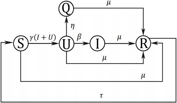
FIGURE 1. The transfer diagram of a system.

TABLE 1

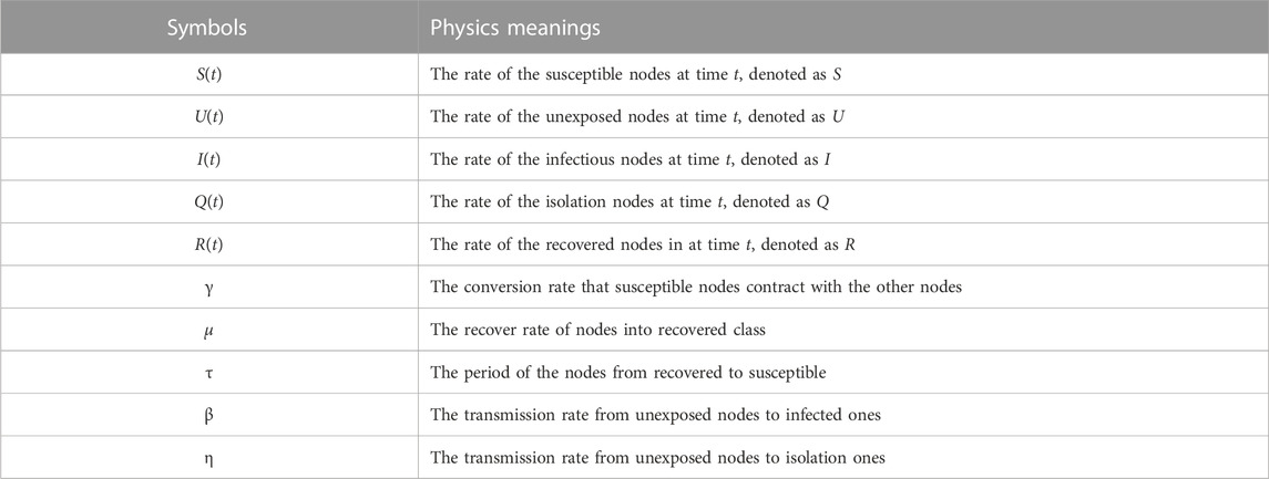
TABLE 1. Definition of the parameters.

The susceptible nodes will be infected by the unexposed nodes and infectious nodes at the rate of γ. There are γS(U + I) nodes, which will remove from class S into class U. Due to the system being updated at a certain period, the nodes in WSNs will enter the class R at the rate of μ. The recovered nodes will enter class S at the rate of τ due to protection failure [26, 27]. Therefore, the transfer relationships between S and other classes can be expressed as follows:

$\frac{dS}{dt}=-\gamma S\left(U+I\right)+\tau R-\mu S.(2)$

The density of the unexposed nodes will increase when the susceptible nodes are infected. Some unexposed nodes will be found as the isolated class Q at the rate of η through regular checking. Some unexposed nodes will move into class I before being recovered at the rate of β. Therefore, the transfer relationships between U and other classes can be expressed as follows:

$\frac{dU}{dt}=\gamma S\left(U+I\right)-\mu U-\beta U-\eta U.(3)$

The density of the infectious nodes will increase because some unexposed nodes will move into class I. Some nodes in class I will remove into class R due to the periodic system updates at the rate of μ. Therefore, the transfer relationships between I and other classes can be expressed as the following equations:

$\frac{dI}{dt}=\beta U-\mu I,(4)$

The density of the isolation nodes will increase when the unexposed nodes are founded. Some nodes in class Q will remove into class R due to the periodic system updates at the rate of μ. Therefore, the transfer relationships between Q and other classes can be expressed as the following equations:

$\frac{dQ}{dt}=\eta U-\mu Q.(5)$

Assuming the total number of the nodes in WSNs is a constant. Therefore, the transfer relationships between R and other classes can be obtained as follows:

$\frac{dR}{dt}=\mu S+\mu U+\mu I+\mu Q-\tau R.(6)$

Combining the above ideas, the SUIQR model governing the transmission of malware is described by the following system of non-linear differential equations:

$\left\{\begin{array}{c}\frac{\partial S}{\partial t}=-\gamma S\left(U+I\right)+\tau R-\mu S,\hfill \\ \frac{\partial U}{\partial t}=\gamma S\left(U+I\right)-\mu U-\beta U-\eta U,\hfill \\ \frac{\partial I}{\partial t}=\beta U-\mu I,\hfill \\ \frac{\partial Q}{\partial t}=\eta U-\mu Q,\hfill \\ \frac{\partial R}{\partial t}=\mu S+\mu U+\mu I+\mu Q-\tau R.\hfill \end{array}\right.(7)$

3 The mathematical analysis of the SUIQR epidemic model

The basic reproductive number is a key parameter to represent the infected numbers in an average infection period. Firstly, the global stability of the malware-free equilibrium (MFE) is introduced [28]. We can get the SUIQR model 7) to have a malware-free equilibrium point $P_f^{*}$ and the malware-endemic equilibrium point $P_e^{*}$ by solving the following Eq. 8:

$\left\{\begin{array}{c}-\gamma S\times \left(U+I\right)+\tau R-\mu S=0,\hfill \\ \gamma S\times \left(U+I\right)-\mu U-\beta U-\eta U=0,\hfill \\ \beta U-\mu I=0,\hfill \\ \eta U-\mu Q=0,\hfill \\ S+U+R+I+Q=1.\hfill \end{array}\right.(8)$

The malware-free equilibrium point $P_f^{*}$ and the malware-endemic equilibrium point $P_e^{*}$ are shown in Eq.9 and Eq.(10), respectively:

$P_f^{*}\left(S_f^{*},U_f^{*},I_f^{*},Q_f^{*},R_f^{*}\right)=\left(\frac{\tau }{\mu +\tau },\mathrm{0,0,0},\frac{\mu }{\mu +\tau }\right).(9)$

$\begin{array}{cc}\hfill P_e^{\ast }\left(S_e^{\ast },U_e^{\ast },I_e^{\ast },Q_e^{\ast },R_e^{\ast }\right)=& \left(\frac{\beta \mu +\eta \mu +{\mu }^2}{\beta \gamma +\gamma \mu },-\frac{\mu \left(\beta {\mu }^2+\eta {\mu }^2+{\mu }^2\tau +{\mu }^3-\beta \gamma \tau +\beta \mu \tau +\eta \mu \tau -\gamma \mu \tau \right)}{\left(\mu +\tau \right)\left(\gamma {\beta }^2+2\gamma \beta \mu +\eta \gamma \beta +\gamma {\mu }^2+\eta \gamma \mu \right)},\right.\hfill \\ \hfill & -\frac{\beta \left(\beta {\mu }^2+\eta {\mu }^2+{\mu }^2\tau +{\mu }^3-\beta \gamma \tau +\beta \mu \tau +\eta \mu \tau -\gamma \mu \tau \right)}{\left(\mu +\tau \right)\left(\gamma {\beta }^2+2\gamma \beta \mu +\eta \gamma \beta +\gamma {\mu }^2+\eta \gamma \mu \right)},\hfill \\ \hfill & \left.-\frac{\eta {\mu }^3+{\eta }^2{\mu }^2+\eta {\mu }^2\tau +{\eta }^2\mu \tau +\beta \eta {\mu }^2-\beta \eta \gamma \tau +\beta \eta \mu \tau -\eta \gamma \mu \tau }{\left(\mu +1\right)\left(\gamma {\beta }^2+2\gamma \beta \mu +\eta \gamma \beta +\gamma {\mu }^2+\eta \gamma \mu \right)},\frac{\mu }{\mu +\tau }\right)\hfill \end{array}(10)$

Then, the next-generation method (NGM) is applied to calculate the basic reproductive number R₀ [29]. The main advantage of the NGM is that it allows the research to ignore any uninfected classes and focus only on the infected classes. There are three infected classes in the proposed SUIQR model. Let X = (U,I,Q)^T, the model 7) equals to the following form:

$\frac{dX}{dt}=F-V.(11)$

Where $F=\left(\begin{array}{c}\hfill \gamma S(U+I)\hfill \\ \hfill 0\hfill \\ \hfill 0\hfill \end{array}\right)$ and $V=\left(\begin{array}{c}\hfill \mu U+\beta U+\eta U\hfill \\ \hfill -\beta U+\mu I\hfill \\ \hfill -\eta U+\mu Q\hfill \end{array}\right)$.

We define f and v as the Jacobian matrices of F and V evaluated at the malware-free equilibrium point $P_f^{*}$:

$f=\left(\frac{\partial F}{\partial X}\right){|}_{P_f^{*}}=\left(\begin{array}{ccc}\hfill \gamma S_f^{*}\hfill & \hfill \gamma S_f^{*}\hfill & \hfill 0\hfill \\ \hfill 0\hfill & \hfill 0\hfill & \hfill 0\hfill \\ \hfill 0\hfill & \hfill 0\hfill & \hfill 0\hfill \end{array}\right)=\left(\begin{array}{ccc}\hfill \frac{\tau \gamma }{\mu +\tau }\hfill & \hfill \frac{\tau \gamma }{\mu +\tau }\hfill & \hfill 0\hfill \\ \hfill 0\hfill & \hfill 0\hfill & \hfill 0\hfill \\ \hfill 0\hfill & \hfill 0\hfill & \hfill 0\hfill \end{array}\right).(12)$

$v=\left(\frac{\partial V}{\partial X}\right){|}_{P_f^{*}}=\left(\begin{array}{ccc}\hfill \mu +\beta +\eta \hfill & \hfill 0\hfill & \hfill 0\hfill \\ \hfill -\beta \hfill & \hfill \mu \hfill & \hfill 0\hfill \\ \hfill -\eta \hfill & \hfill 0\hfill & \hfill \mu \hfill \end{array}\right).(13)$

The basic reproductive number R₀ is the largest eigenvalue of the matrix fv⁻¹ given by Eq. 14:

$f{v}^{-1}=\left(\begin{array}{cccc}\hfill \frac{\left(\beta +\mu \right)\tau \gamma }{\mu \left(\mu +\tau \right)\left(\beta +\eta +\mu \right)}\hfill & \hfill \frac{\gamma \tau }{\mu \left(\mu +\tau \right)}\hfill & \hfill 0\hfill & \hfill \hfill \\ \hfill 0\hfill & \hfill 0\hfill & \hfill 0\hfill \\ \hfill 0\hfill & \hfill 0\hfill & \hfill 0\hfill \end{array}\right).(14)$

Then, we can obtain the basic reproductive number R₀.

$R_0=\rho \left(f{v}^{-1}\right)=\frac{\left(\beta +\mu \right)\tau \gamma }{\mu \left(\mu +\tau \right)\left(\beta +\eta +\mu \right)}.(15)$

When R₀ < 1, it means that the SUIQR model will reach a malware-free situation eventually; when R₀ > 1, the SUIQR model always has malware and has an endemic equilibrium.

Finally, we analyze the sensitivity of each parameter (μ, η, β, λ) about the basic reproductive number and obtain normed forward sensitivity indexes as follows:

$\left\{\begin{array}{c}\frac{\frac{\partial R_0}{R_0}}{\frac{\partial \lambda }{\lambda }}=1>0,\hfill \\ \frac{\frac{\partial R_0}{R_0}}{\frac{\partial \beta }{\beta }}=\frac{\eta \beta }{\left(\beta +\mu \right)\left(\beta +\mu +\eta \right)}>0,\hfill \\ \frac{\frac{\partial R_0}{R_0}}{\frac{\partial \mu }{\mu }}=\frac{\tau \gamma \left({\mu }^2+\mu \tau \right)\left(\beta +\eta +\mu \right)-\tau \gamma \left(\beta +\mu \right)\left(3{\mu }^2+2\mu \left(\beta +\eta +\tau \right)+\tau \beta +\tau \eta \right)}{\left(\mu +\tau \right)\left(\beta +\eta +\mu \right)\left(\beta +\mu \right)\tau \gamma }<0,\hfill \\ \frac{\frac{\partial R_0}{R_0}}{\frac{\partial \eta }{\eta }}=\frac{-\eta }{\beta +\mu +\eta }<0.\hfill \end{array}\right.(16)$

It is obvious that λ, β and R₀ are proportional, η, μ, and R₀ are inverse proportional. The increase of η or μ may result in the decrease of R₀. The decrease of λ and β may result in the decrease of R₀. Above all, we can take some measures to control the spread of malware.

• Reduce the period of system updates. This can improve the defense capabilities of nodes, that is, to increase μ.

• Reduce the communication frequency between nodes, that is, to decrease λ. This will reduce the conversion rate that susceptible nodes contract with the other nodes.

The Jacobian matrix of the SUIQR model at $P_e^{*}$ is as follows:

$J=\left(\begin{array}{ccccc}\hfill -\gamma \left(U_e^{\ast }+I_e^{\ast }\right)-\mu \hfill & \hfill -\gamma S_e^{\ast }\hfill & \hfill -\gamma S_e^{\ast }\hfill & \hfill 0\hfill & \hfill \tau \hfill \\ \hfill \gamma \left(U_e^{\ast }+I_e^{\ast }\right)\hfill & \hfill \gamma S_e-\mu -\beta -\eta \hfill & \hfill \gamma S_e\hfill & \hfill 0\hfill & \hfill 0\hfill \\ \hfill 0\hfill & \hfill \beta \hfill & \hfill -\mu \hfill & \hfill 0\hfill & \hfill 0\hfill \\ \hfill 0\hfill & \hfill \eta \hfill & \hfill 0\hfill & \hfill -\mu \hfill & \hfill 0\hfill \\ \hfill \mu \hfill & \hfill \mu \hfill & \hfill \mu \hfill & \hfill \mu \hfill & \hfill -\tau \hfill \end{array}\right).(17)$

The corresponding characteristic equation is shown in Eq. 18:

${\lambda }^5+A_4{\lambda }^4+A_3{\lambda }^3+A_2{\lambda }^2+A_1\lambda +A_0=0.(18)$

$\left\{\begin{array}{c}\begin{array}{cc}\hfill A_4=& \beta +\eta +4\mu -\tau +\gamma I_e^{\ast }-\gamma S_e^{\ast }+\gamma U_e^{\ast },\hfill \\ \hfill A_3=& 3\beta \mu +3\eta \mu -\beta \tau -\eta \tau -5\mu \tau +6{\mu }^2+\beta \gamma I_e^{\ast }+\eta \gamma I_e^{\ast }-\beta \gamma S_e^{\ast }+3\gamma \mu I_e^{\ast }+\beta \gamma U_e^{\ast }+\eta \gamma U_e^{\ast }\hfill \\ \hfill & -\gamma \tau I_e^{\ast }-3\gamma \mu S_e^{\ast }+3\gamma \mu U_e^{\ast }+\gamma \tau S_e^{\ast }-\gamma \tau U_e^{\ast },\hfill \\ \hfill A_2=& 3\beta {\mu }^2+3\eta {\mu }^2-9{\mu }^2\tau +4{\mu }^3-4\beta \mu \tau -4\eta \mu \tau +3\gamma {\mu }^2{I}_e^{\ast }-3\gamma {\mu }^2{S}_e^{\ast }+3\gamma {\mu }^2{U}_e^{\ast }+2\beta \gamma \mu I_e^{\ast }\hfill \\ \hfill & +2\eta \gamma \mu I_e^{\ast }-\beta \gamma \tau I_e^{\ast }-2\beta \gamma \mu S_e^{\ast }-\eta \gamma \tau I_e^{\ast }+2\beta \gamma \mu U_e^{\ast }+2\eta \gamma \mu U_e^{\ast }+\beta \gamma \tau S_e^{\ast }-4\gamma \mu \tau I_e^{\ast }\hfill \\ \hfill & -\beta \gamma \tau U_e^{\ast }-\eta \gamma \tau U_e^{\ast }+4\gamma \mu \tau S_e^{\ast }-4\gamma \mu \tau U_e^{\ast },\hfill \\ \hfill A_1=& \beta {\mu }^3+\eta {\mu }^3-7{\mu }^3\tau +{\mu }^4-5\beta {\mu }^2\tau -5\eta {\mu }^2\tau +\gamma {\mu }^3{I}_e^{\ast }-\gamma {\mu }^3{S}_e^{\ast }+\gamma {\mu }^3{U}_e^{\ast }+\beta \gamma {\mu }^2{I}_e^{\ast }\hfill \\ \hfill & +\eta \gamma {\mu }^2{I}_e^{\ast }-\beta \gamma {\mu }^2{S}_e^{\ast }+\beta \gamma {\mu }^2{U}_e^{\ast }+\eta \gamma {\mu }^2{U}_e^{\ast }-5\gamma {\mu }^2\tau I_e^{\ast }+5\gamma {\mu }^2\tau S_e^{\ast }-5\gamma {\mu }^2\tau U_e^{\ast }\hfill \\ \hfill & -3\beta \gamma \mu \tau I_e^{\ast }-3\eta \gamma \mu \tau I_e^{\ast }+3\beta \gamma \mu \tau S_e^{\ast }-3\beta \gamma \mu \tau U_e^{\ast }-3\eta \gamma \mu \tau U_e^{\ast },\hfill \\ \hfill A_0=& 2\gamma {\mu }^3\tau S_e^{\ast }-2\beta {\mu }^3\tau -2\eta {\mu }^3\tau -2\gamma {\mu }^3\tau I_e^{\ast }-2{\mu }^4\tau -2\gamma {\mu }^3\tau U_e^{\ast }-2\beta \gamma {\mu }^2\tau I_e^{\ast }-2\eta \gamma {\mu }^2\tau I_e^{\ast }\hfill \\ \hfill & +2\beta \gamma {\mu }^2\tau S_e^{\ast }-2\beta \gamma {\mu }^2\tau U_e^{\ast }-2\eta \gamma {\mu }^2\tau U_e^{\ast }.\hfill \end{array}\hfill \end{array}\right.(19)$

According to the Routh-Hurwitz criterion [27], when R₀ > 1, the endemic equilibrium $P_e^{*}\left(\right.S_e^{*},U_e^{*}$, $I_e^{*},Q_e^{*},R_e^{*}\left.\right)$ is asymptotically stable.

4 The optimal control strategy

We assume that the distribution of the nodes follows the Poisson point process in WSN. The probability of there being k nodes in the communication range can be calculated by the following equation (30):

$P\left\{X=k\right\}=\frac{{\left(\lambda \pi R_1^2\right)}^k{e}^{-\lambda \pi R_1^2}}{k!}.(20)$

Where λ is the density of the nodes in WSNs, and R₁ is the communication range of each node, which is always an adjustable parameter.

Therefore, the conversion rate that susceptible nodes contract with the other nodes can be calculated by the following equation:

$\gamma =E\left(X\right)=\lambda \pi R_1^2.(21)$

The sensitivity of the communication range about the basic reproductive number and obtaining a normed forward sensitivity index is shown as Eq. 22:

$\frac{\frac{\partial R_0}{R_0}}{\frac{\partial R_1}{R_1}}=\frac{2}{R_1}>0.(22)$

According to the analysis above, we need to adjust the parameters (μ or R₁) to keep the basic reproductive number at less than 1. By substituting Eq. 21 into Eq. 15, the relationship between μ and R₁ is given by the following inequality:

$\frac{\left(\beta +\mu \right)\tau \lambda \pi R_1^2}{\mu \left(\mu +\tau \right)\left(\beta +\eta +\mu \right)}<1.(23)$

•Case 1. R₁ is the adjustable parameter and μ is the fixed constant:

$R_1<\sqrt{\frac{\mu \left(\mu +\tau \right)\left(\beta +\eta +\mu \right)}{\left(\beta +\mu \right)\tau \lambda \pi }}.(24)$

Based on the above inequality, we set the threshold of the communication range. When the range is less than the threshold, the SUIQR model reaches a malware-free situation eventually.

•Case 2. μ is the adjustable parameter and R₁ is the fixed constant:

${\mu }^3+\left(\beta +\eta +\tau \right){\mu }^2+\left(\tau \beta +\tau \eta -\tau \lambda \pi R_1^2\right)\mu -\tau \lambda \pi \beta R_1^2>0.(25)$

5 Numerical simulations

In this section, some numerical simulations are performed to illustrate and complement our analytical results. There are 100 nodes in the networks with the area of 1000 × 1000. We fix the parameters β = 0.6, λ = 0.0001, η = 0.3, μ = 0.1, R₁ = 50, τ = 0.3. The initial density of each class is S(0) = 0.6, U(0) = 0.1, I(0) = 0.1, Q(0) = 0.1, R(0) = 0.1. The evolutions of each class along with time are shown in Figure 2.

FIGURE 2

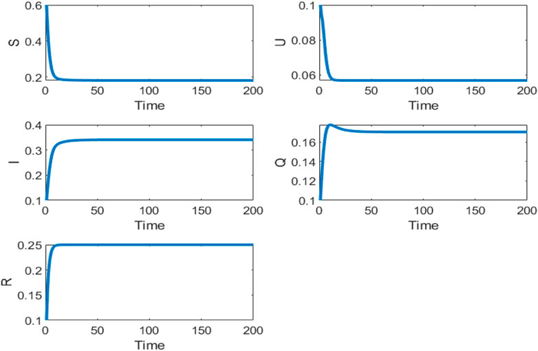
FIGURE 2. Evolutions of S, U, I, Q, R along with time t.

In this example, we can calculate the basic reproductive number R₀ = 4.1233 based on Eq. 15 As can be seen from Figure 2, the reproduction number is determined by R₀ > 1. Here, we can see the densities of class S and class U decrease rapidly over time and eventually stabilize the equilibrium point $P_e^{*}$, with a high rate of conversion and recovery. The densities of class I and class R increase rapidly over time and eventually stabilize the equilibrium point. The malware-endemic equilibrium point $P_e^{*}=[0.1819,0.0568,0.3409,0.2500]$. The malware will exist in this WSN. The corresponding characteristic equation is shown as follows:

${\lambda }^5+2.5406{\lambda }^4+2.0997{\lambda }^3+0.6419{\lambda }^2+0.0692\lambda +0.0024=0(26)$

The roots of the characteristic equation are [-1.1874, −0.8467, - 0.3370, −0.1000, −0.0695]. The Routh-Hurwitz table is given by:

$H=\left(\begin{array}{ccc}\hfill 1.0000\hfill & \hfill 2.0997\hfill & \hfill 0.0692\hfill \\ \hfill 2.5406\hfill & \hfill 0.6419\hfill & \hfill 0.0024\hfill \\ \hfill 1.8470\hfill & \hfill 0.0683\hfill & \hfill 0\hfill \\ \hfill 0.5480\hfill & \hfill 0.0024\hfill & \hfill 0\hfill \\ \hfill 0.0603\hfill & \hfill 0\hfill & \hfill 0\hfill \\ \hfill 0.0024\hfill & \hfill 0\hfill & \hfill 0\hfill \end{array}\right).$

According to the Routh-Hurwitz criterion, this system is stable based on the given parameters.

Then, we analyze the influence of the optimal control strategy on the evolutions of each class. In the above example, the malware will not be eliminated. When only one parameter is adjustable, R₁ can be calculated by Eq.24, R₁ < 24.6233 if R₀ < 1. We fixed R₁ = 24, and the evolutions of each class are shown in Figure 3.

FIGURE 3

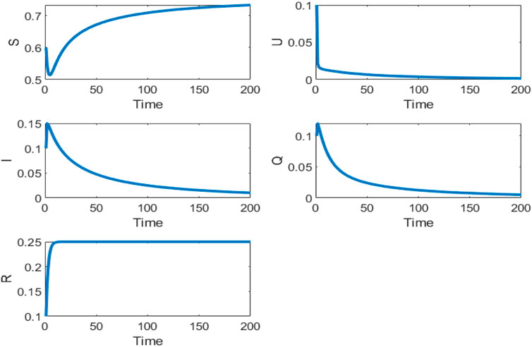
FIGURE 3. Evolutions of S, U, I, Q, R for τ =2, R₁=24, μ =0.1 along with time t.

In this example, we can calculate the basic reproductive number R₀ = 0.9500 based on Eq. 15 As can be seen from Figure 3, the reproduction number is determined by R₀ < 1. Here, the densities of class S, class U, and class Q can be seen to increase rapidly and decay slowly to 0, with a high recovery rate. The density of class S decreases rapidly and then slowly increases to eventually stabilize the equilibrium point. The malware-free equilibrium point $P_f^{*}=[0.75,\mathrm{0,0,0,0.25}]$. The corresponding characteristic equation is shown as follows:

${\lambda }^5+1.6188{\lambda }^4+0.5099{\lambda }^3+0.2729{\lambda }^2-0.0012\lambda -0.00003=0(27)$

The roots of the characteristic equation are [-1.2197, −0.3179, −0.1000, 0.0391, −0.0202]. The Routh-Hurwitz table is given by:

$H=\left(\begin{array}{ccc}\hfill 1.0000\hfill & \hfill 0.5099\hfill & \hfill -0.0012\hfill \\ \hfill 1.6188\hfill & \hfill 0.0273\hfill & \hfill -0.0000\hfill \\ \hfill 0.4930\hfill & \hfill -0.0011\hfill & \hfill 0\hfill \\ \hfill 0.0310\hfill & \hfill -0.0000\hfill & \hfill 0\hfill \\ \hfill -0.0007\hfill & \hfill 0\hfill & \hfill 0\hfill \\ \hfill -0.0000\hfill & \hfill 0\hfill & \hfill 0\hfill \end{array}\right).$

According to the Routh-Hurwitz criterion, this system is stable based on the given parameters.

When only one parameter is adjustable, μ can be calculated by Eq. 24, μ > 0.2961. We fixed the communication range of each R₁ = 0.3, and the evolutions of each class are shown in Figure 4.

FIGURE 4

FIGURE 4. Evolutions of S, U, I, Q, R for τ =2, R₁=50, μ =0.4 along with time t.

In this example, we can calculate the basic reproductive number R₀ = 0.9817 based on Eq. 15 As can be seen from Figure 4, it is observed that the reproduction number is determined by R₀ < 1. Here, the densities of class S, class U, and class Q can be seen to increase rapidly and decay slowly to 0, with a high recovery rate. The density of class S decreases rapidly and then slowly increases to eventually stabilize the equilibrium point. The SUIQR model will reach a malware-free situation eventually, and the malware-free equilibrium point $P_f^{*}=[0.5,\mathrm{0,0,0,0.5}]$. The corresponding characteristic equation is shown as follows:

${\lambda }^5+3.2799{\lambda }^4+3.3250{\lambda }^3+1.2538{\lambda }^2-0.1903\lambda -0.0099=0(28)$

The roots of the characteristic equation are [-1.7649, −0.9278, −0.3000, −0.1658, −0.1214]. The Routh-Hurwitz table is given by:

$H=\left(\begin{array}{ccc}\hfill 1.0000\hfill & \hfill 3.3250\hfill & \hfill 0.1903\hfill \\ \hfill 3.2799\hfill & \hfill 1.2538\hfill & \hfill 0.0099\hfill \\ \hfill 2.9427\hfill & \hfill 0.1873\hfill & \hfill 0\hfill \\ \hfill 1.0450\hfill & \hfill 0.0099\hfill & \hfill 0\hfill \\ \hfill 0.1594\hfill & \hfill 0\hfill & \hfill 0\hfill \\ \hfill 0.0099\hfill & \hfill 0\hfill & \hfill 0\hfill \end{array}\right).$

According to the Routh-Hurwitz criterion, this system is stable based on the given parameters.

We set the update period of the system μ, which satisfies the above inequality to ensure the SUIQR model will reach a malware-free situation eventually. As shown in Figures 3, 4, the system is optimal and stable when the R₁ or μ is set. We can obtain the control strategy to reduce the spread of malware by setting reasonable parameters for nodes in WSNs.

Sometimes, the results of adjusting the single parameter μ or R₁ are not satisfactory. In these scenes, we need to adjust μ and R₁ simultaneously; the relationship between μ and R₁ is given in Eq. 25 Based on the given parameters, the relationship between the two parameters is shown in Figure 5.

FIGURE 5

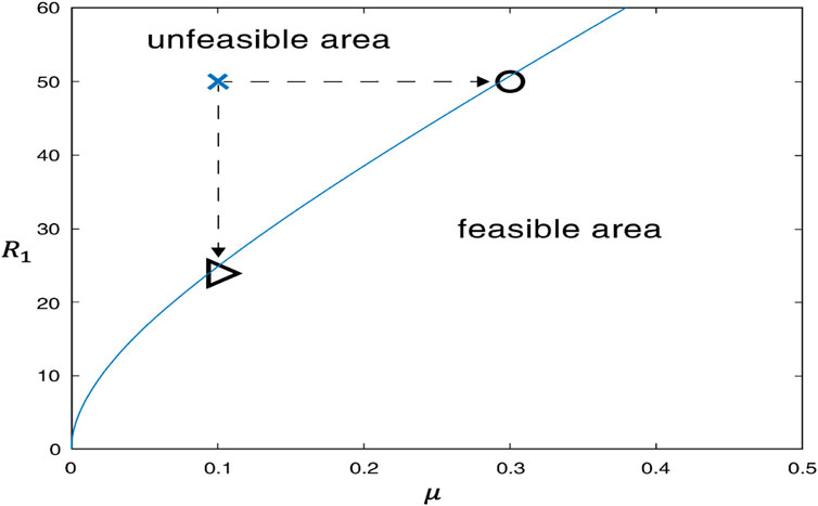
FIGURE 5. Evolutions of S, U, I, Q, R along with time t.

As shown in Figure 5, the region below is feasible, while the region above is not. We can adjust these two parameters in the curve to ensure the SUIQR model reaches a malware-free situation eventually. A schematic of the results of controlling both the communication radius and the frequency of system updates to the system is shown in Figure 5. The previous control method highlights that malware propagation in networks can be simulated regardless of whether the radius of communication is decreased or the frequency of updates to the system is increased. In the curve shown in Figure 5, the entire space is divided into two parts. The upper part of the space is not feasible, that is, the control strategy in the upper part of the space cannot achieve the purpose of suppressing the spread of malware. The second half of the space is the feasible part, that is, the control strategy in the second half of the space can effectively suppress the malware. The points on the curve represent the critical values and are the most up-to-date regulatory solution. If the current control strategy can fail to achieve the goal of suppressing malware propagation, control can be achieved by adjusting the radius of communication at a triangle checkpoint or by increasing the frequency of system updates at the circle checkpoint.

6 Conclusion

This article proposed a SUIQR epidemic model to describe the spreading of malware. The basic reproductive number was derived by using the next-generation method. Finally, we carried out numerical simulations to observe the malware spreading in WSNs to verify the obtained theoretical results. Furthermore, we also investigated the communication range of the nodes to make the results more complete. As a result, we can adjust the communication range and the period of system updating to reduce the spreading of malware in WSNs. Due to the lack of experimental data, only numerical simulations were performed in this article, which is also a limitation of the work. In our further work, we will continue to investigate and perform relevant experiments and compare them with other infectious disease models to verify that the method is feasible.

Data availability statement

The original contributions presented in the study are included in the article/Supplementary Material, further inquiries can be directed to the corresponding authors.

Author contributions

YZ: Writing-original draft; YW: Undertook the data analysis; KZ: Methodology; SF-S: Writing-reviewing and editing; W-XM: Writing-reviewing and editing.

Funding

Funding was provided by the National Natural Science Foundation of China (Grant Nos. 11871336, 11771395).

Acknowledgments

We would like to express our sincere thanks to the referees for their useful comments and timely help.

Conflict of interest

The authors declare that the research was conducted in the absence of any commercial or financial relationships that could be construed as a potential conflict of interest.

Publisher’s note

All claims expressed in this article are solely those of the authors and do not necessarily represent those of their affiliated organizations, or those of the publisher, the editors and the reviewers. Any product that may be evaluated in this article, or claim that may be made by its manufacturer, is not guaranteed or endorsed by the publisher.

References

1. Kephart JO, White SR Proceedings of the IEEE computer society symposium research in security and privacy (1991). p. 343–59.

Google Scholar

2. Youssef M, Scoglio C An individual-based approach to SIR epidemics in contact networks. J Theor Biol (2011) 283(1):136–44. doi:10.1016/j.jtbi.2011.05.029

PubMed Abstract | CrossRef Full Text | Google Scholar

3. Feng L, Liao X, Han Q, Li H Dynamical analysis and control strategies on malware propagation model. Appl Math Model (2013) 37(16-17):8225–36. doi:10.1016/j.apm.2013.03.051

CrossRef Full Text | Google Scholar

4. del Rey AM, Vara RC, González SR A computational propagation model for malware based on the SIR classic model. Neurocomputing (2022) 484:161–71. doi:10.1016/j.neucom.2021.08.149

CrossRef Full Text | Google Scholar

5. Xiao M, Chen S, Zheng WX, Wang Z, Lu Y Tipping point prediction and mechanism analysis of malware spreading in cyber–physical systems. Commun Nonlinear Sci Numer Simulation (2023) 122:107247. doi:10.1016/j.cnsns.2023.107247

CrossRef Full Text | Google Scholar

6. Dong NP, Long HV, Son NTK The analysis of a fractional network-based epidemic model with saturated treatment function and fuzzy transmission. Iranian J Fuzzy Syst (2023) 20(1):1–18. doi:10.22111/ijfs.2023.7342

CrossRef Full Text | Google Scholar

7. Carnier RM, Li Y, Fujimoto Y, Shikata J Modeling exact Markov chains for malware based on random propagation. Techrxiv Techrxiv (2023). doi:10.36227/techrxiv.22047527

CrossRef Full Text | Google Scholar

8. Prajapati A International conference on cybersecurity, cybercrimes, and smart emerging technologies (CCSET), riyadh. SAUDI ARABIA (2022). Paper presented at the.May 10-11) A Propagation Model of Malicious Objects via Removable Devices and Sensitivity Analysis of the Parameters

Google Scholar

9. Liu J, Saeed T, Zeb A Delay effect of an e-epidemic SEIRS malware propagation model with a generalized non-monotone incidence rate. Results Phys (2022) 39:105672. doi:10.1016/j.rinp.2022.105672

CrossRef Full Text | Google Scholar

10. Shakya RK, Rana K, Gaurav A, Mamoria P, Srivastava PK Stability analysis of epidemic modeling based on spatial correlation for wireless sensor networks. Wireless Personal Commun (2019) 108(3):1363–77. doi:10.1007/s11277-019-06473-0

CrossRef Full Text | Google Scholar

11. JiPar LPE, NediTang ACY, Baar T, Basar T. On the analysis of a continuous-time Bi-virus model. Ieee Trans Automatic Control (2016) 64(12):4891–906. doi:10.1109/CDC.2016.7798284

CrossRef Full Text | Google Scholar

12. Zhang Z, Kumari S, Upadhyay RK A delayed e-epidemic SLBS model for computer virus. Adv Difference Equations (2019) 2019(1):414. doi:10.1186/s13662-019-2341-8

CrossRef Full Text | Google Scholar

13. Yu Z, Gao H, Wang D, Alnuaim AA, Firdausi M, Mostafa AM SEI2RS malware propagation model considering two infection rates in cyber-Cphysical systems. Physica A: Stat Mech its Appl (2022) 597:127207. doi:10.1016/j.physa.2022.127207

CrossRef Full Text | Google Scholar

14. Fedorov D, Tabarak Y, Dadlani A, Kumar MS, Kizheppatt V Dynamics of multi-strain malware epidemics over duty-cycled wireless sensor networks. In: 2021 International Balkan Conference on Communications and Networking (BalkanCom) (2021). p. 1–5. doi:10.1109/BalkanCom53780.2021.9593147

CrossRef Full Text | Google Scholar

15. Dong NP, Long HV, Son NTK The dynamical behaviors of fractional-order SE1E2IQR epidemic model for malware propagation on Wireless Sensor Network. Commun Nonlinear Sci Numer Simulation (2022) 111:106428. doi:10.1016/j.cnsns.2022.106428

CrossRef Full Text | Google Scholar

16. Dong NP, Long HV, Khastan A Optimal control of a fractional order model for granular SEIR epidemic with uncertainty. Commun Nonlinear Sci Numer Simulation (2020) 88:105312. doi:10.1016/j.cnsns.2020.105312

PubMed Abstract | CrossRef Full Text | Google Scholar

17. Nwokoye CH, Madhusudanan V, Srinivas MN, Mbeledogu NN Modeling time delay, external noise and multiple malware infections in wireless sensor networks. Egypt Inform J (2022) 23(2):303–14. doi:10.1016/j.eij.2022.02.002

CrossRef Full Text | Google Scholar

18. Ojha RP, Srivastava PK, Sanyal G, Gupta N Improved model for the stability analysis of wireless sensor network against malware attacks. Wireless Personal Commun (2020) 116(3):2525–48. doi:10.1007/s11277-020-07809-x

CrossRef Full Text | Google Scholar

19. Hosseini S, Azgomi MA The dynamics of an SEIRS-QV malware propagation model in heterogeneous networks. Physica A: Stat Mech its Appl (2018) 512:803–17. doi:10.1016/j.physa.2018.08.081

CrossRef Full Text | Google Scholar

20. Hosseini S, Azgomi MA Dynamical analysis of a malware propagation model considering the impacts of mobile devices and software diversification. Physica A: Stat Mech its Appl (2019) 526:120925. doi:10.1016/j.physa.2019.04.161

CrossRef Full Text | Google Scholar

21. Hosseini S, Azgomi MA A model for malware propagation in scale-free networks based on rumor spreading process. Computer Networks (2016) 108:97–107. doi:10.1016/j.comnet.2016.08.010

CrossRef Full Text | Google Scholar

22. Muthukrishnan S, Muthukumar S, Chinnadurai V Optimal control of malware spreading model with tracing and patching in wireless sensor networks. Wireless Personal Commun (2020) 117(3):2061–83. doi:10.1007/s11277-020-07959-y

CrossRef Full Text | Google Scholar

23. Liu W, Zhong S (2017). Web malware spread modelling and optimal control strategies. Sci Rep, 7, 42308. doi:10.1038/srep42308

PubMed Abstract | CrossRef Full Text | Google Scholar

24. Nwokoye CH, Madhusudanan V Epidemic models of malicious-code propagation and control in wireless sensor networks: An indepth review. Wireless Personal Commun (2022) 125(2):1827–56. doi:10.1007/s11277-022-09636-8

CrossRef Full Text | Google Scholar

25. Jain A, Dhar J, Gupta VK Optimal control of rumor spreading model on homogeneous social network with consideration of influence delay of thinkers. Differential Equations Dynamical Syst (2019) 31(1):113–34. doi:10.1007/s12591-019-00484-w

CrossRef Full Text | Google Scholar

26. Yang F, Zhang Z Hopf bifurcation analysis of SEIR-KS computer virus spreading model with two-delay. Results Phys (2021) 24:104090. doi:10.1016/j.rinp.2021.104090

CrossRef Full Text | Google Scholar

27. Zhang H, Upadhyay RK, Liu G, Zhang Z Hopf bifurcation and optimal control of a delayed malware propagation model on mobile wireless sensor networks. Results Phys (2022) 41:105926. doi:10.1016/j.rinp.2022.105926

CrossRef Full Text | Google Scholar

28. Wei X, Xu G, &Zhou W Global stability of endemic equilibrium for a SIQRS epidemic model on complex networks Physica A: Stat Mech its Appl (2018) 512:203–14. doi:10.1016/j.physa.2018.08.119

CrossRef Full Text | Google Scholar

29. Posny D, Wang J Computing the basic reproductive numbers for epidemiological models in nonhomogeneous environments. Appl Maths Comput (2014) 242:473–90. doi:10.1016/j.amc.2014.05.079

CrossRef Full Text | Google Scholar

30. Habibiyan R, Ghorban Sabbagh A Connectivity analysis of 2D underwater optical wireless sensor networks using a geometric approach. Ad Hoc Networks (2022) 134:102910. doi:10.1016/j.adhoc.2022.102910

CrossRef Full Text | Google Scholar