 Bolun Chen1,2
 Shuai Han
95% of researchers rate our articles as excellent or good
Learn more about the work of our research integrity team to safeguard the quality of each article we publish.
Find out more
ORIGINAL RESEARCH article
Front. Phys. , 04 October 2023
Sec. Complex Physical Systems
Volume 11 - 2023 | https://doi.org/10.3389/fphy.2023.1195087
This article is part of the Research Topic Mathematical modeling and optimization for real life phenomena View all 11 articles
In recent years, coronavirus disease 2019 (COVID-19) has plagued the world, causing huge losses to the lives and property of people worldwide. How to simulate the spread of an epidemic with a reasonable mathematical model and then use it to analyze and to predict its development trend has attracted the attention of scholars from different fields. Based on the susceptible–infected–recovered (SIR) propagation model, this work proposes the susceptible–exposed–infected–recovered–dead (SEIRD) model by introducing a specific medium having many changes such as the self-healing rate, lethality rate, and re-positive rate, considering the possibility of virus propagation through objects. Finally, this work simulates and analyzes the propagation process of nodes in different states within this model, and compares the model prediction results optimized by the adaptive genetic algorithm with the real data. The experimental results show that the susceptible–exposed–infected–recovered–dead model can effectively reflect the real epidemic spreading process and provide theoretical support for the relevant prevention and control departments.
Epidemic transmission is the spread of various infectious diseases between different individuals and in most cases endangers human health and safety. For example, the recent emergence of COVID-19 was caused by an epidemic virus that spread rapidly worldwide due to its high transmission capacity and difficulty in prevention, resulting in a large number of infected people and deaths, causing significant negative impacts and economic losses in countries worldwide. If trends in the number of infected people are predicted in advance by transmission models and methods, it will make a great contribution to the control of epidemics and the safety of people in all the countries worldwide [1]. Infectious disease models have always been an important basis for studying epidemics, and most scholars from different fields have used infectious disease models to study epidemics. Since the outbreak of COVID-19, the study of epidemic and infectious disease prediction models has once again become a hot topic of research. Due to the existence of certain unknowns and variability of viruses, the factors considered in prediction are gradually increasing, and it is difficult to obtain the complete details of virus infection by model prediction [2]. This paper introduces some other factors to the traditional epidemic model SIR so that the new model can be more applicable to the changes of the actual situation. The addition of latents and deaths to the original model makes the model more accurate in terms of prediction. Infectious disease models focus on the state model and connectivity between individuals; the state model describes the impact of an infected person within a susceptible population in time, while connectivity determines the movement and contact between populations [3]. The variability of the virus can lead to changes in the mode of transmission and make outbreak protection more difficult. Through in-depth understanding of the virus, asymptomatic infections have also been identified in epidemic prevention and control. Such infections carry the transmitted virus but have no significant symptoms and are highly concealed, causing great inconvenience to the protection efforts [4]. With the advancement of medical treatment, self-healing patients have emerged during the treatment process, which also shows that the treatment greatly differs from patient to patient. This work proposes a new prediction model to predict the spread and trend of the epidemic, considering many factor changes, for example, mortality rate, self-healing rate, and repositive rate.
The choice of parameters in the model prediction has a large impact on the prediction results, and the parameter variables will continuously be adjusted using parameter optimization methods so that the prediction results are constantly close to the target values. Genetic algorithms are algorithms that provide optimal or near-optimal solutions to complex problems by simulating natural evolutionary processes. The algorithm uses computer simulation in a mathematical way to convert the process of problem solving into a process similar to the crossover and mutation of chromosomal genes in biological evolution. Adaptive genetic algorithms work better than conventional optimization algorithms in solving complex optimization problems. Therefore, this article uses the adaptive genetic algorithm to optimize the model parameters so that the predicted values of the model are closer to and match with the true values.
Traditional epidemic models are mainly based on the susceptible–infected–recovered (SIR) model for outbreak transmission studies. The traditional model can predict the trend of the number of infections in the short term and provide some theoretical support for subsequent outbreak prediction. The SIR model was proposed in 1927 by two epidemiologists, McKendric and Kenmack, and this model is one of the classical infectious disease models, specifically used to predict the change in the number of populations at different moments after an outbreak [5].
As a classical epidemiological model, many scholars have used the SIR model to predict the trend of infection changes in regional epidemics. [6] used kinetic differential equations for SIR to predict future trends in the development of the epidemic; first, deriving parameter data based on the number of previous infections and recoveries and obtaining the predictions by aggregating the parameters. To verify the validity of the pandemic modeling approach, [7] improved on the traditional SIR model by maintaining consistency in the total population size to ensure that the number of susceptible individuals did not decline monotonically. A final comparative analysis of the modeling data demonstrates that disease transmission can be controlled with appropriate restrictions and strong policies, and likewise, COVID-19 transmission can be controlled in the communities under consideration. One of the most difficult problems in traditional infectious disease models is the presence of a large number of asymptomatic infected individuals. For this reason, [8] improved the SIR model, taking into account asymptomatic or undetected infected individuals in the new model. Furthermore, considering that the previous model took longer time in infectivity and non-isolation, it was somewhat shortened and finally agreed well with the epidemiological data. To study epidemics transmitted within different regions, [9] introduced a new control variable in the SIR model, namely, the effectiveness of the travel blocking operation. The authors also considered an epidemic model based on the vaccination control, using an asymptotic-regressive discrete scheme for numerical analysis, allowing this model to be applied to epidemics that spread within different regions. The exact solution of the classical SIR model is difficult to obtain in most cases, [10] and in order to obtain the exact solution more simply, the authors obtained the exact analytical solution of the model in a parametric form. The main proposals are the display model corresponding to the fixed values of parameters and the proof that numerical solutions can represent analytical solutions, showing that the general solutions of kinetic models can be represented in the exact parametric form. To better account for the dynamic behavior of epidemiology, [11] developed an SIR model with standardized incidence rates and non-linear recovery rates that takes into account the effect of resources available to the public health system. A three-dimensional model for the co-regulation of total population and disease incidence is also presented, explaining the epidemiological causes of endemic complex dynamic behaviors and concluding that adequate public health resources available are essential for epidemic prevention and control. To make the model more stable, [12] developed an epidemiological model of SIR with a latent period and saturation incidence. On the basis of ensuring that the susceptible population satisfies the logistic equation, the incidence rate is set with the susceptible population in a saturated form to find the threshold of whether the disease will die out automatically. According to the experimental results, if the threshold is less than 1, the disease-free equilibrium is globally progressively stable and the disease gradually disappears, whereas if the threshold exceeds 1, the disease does not gradually disappear.
The improved infectious disease model is mainly based on the susceptible–latent–infected–recovered (SEIR) model. The basic model is not applicable for complex epidemic studies in many aspects, and some scholars have improved the SIR model in order to be closer to the real spread of the epidemic, and the new improved SEIR adds latent to the original one, which is infected and carry the epidemic virus but do not have any evident symptoms themselves, and this stage is also known as the latent period.
Against the backdrop of the global outbreak COVID-19, countries worldwide are looking for better ways to curb the spread of the epidemic. [13] treated the functions in the model as fuzzy parameters, constructed the infection rate, recovery rate, etc., then applied the model parameters to the model, and finally used the matrix method to verify the stability of the model. Epidemic models are simplified methods used for describing the transmission of infectious diseases through individuals. To better investigate the predictive effect of models on epidemics and the conditions under which epidemics can spread, [14] applied the basics of models to real diseases, derived steady-state conditions, and showed that viruses spread only when the threshold parameter R exceeds 1. Furthermore, the transmission conditions of viruses were demonstrated by numerical simulations. Epidemic diseases can easily constitute a public safety problem, and in order to investigate whether pandemics will disappear automatically without human control, [15] modified the model by adding pathogen movements and human interventions to the model and using the next-generation matrix approach to determine the basic reproduction number, while solving the values yielded from the final result without strong control measures and social distance control. Since pandemics do not disappear automatically, [16] proposed a new improved model based on real data. This model applied the particle swarm optimization algorithm to estimate system parameters and finally concluded that the parameters of the SEIR model were different in different scenarios. By introducing seasonal and random infection, non-linear dynamics were discovered, and good results were obtained by using the model to demonstrate the real evolution situation. To numerically visualize the results, [17] studied a new stochastic epidemic model and quantified the behavior during an outbreak, then modeled the epidemic using Markov chains, and provided an effective computational program for the development of the distribution of outbreak duration. The expected ratio distribution of the number of individuals in each category of the model is used to study the evolution of the epidemic before it disappears, and the resulting results are visually presented in numbers. As the spread of the epidemic brings serious consequences and to better estimate the current spread of the epidemic and predict the change of the epidemic, [18] proposed a new conceptual mathematical model and took into account the impact of isolation, hospitalization, panic, and anxiety; established the boundary and balance; analyzed its stability; and verified the relevant predictions of the important models through research and comparison. [19] mainly studied the SEIR model with vaccination strategies, which determined the different morbidities of exposed and infected population, and proved the global asymptotically stable result of disease-free equilibrium using the Lyapunov function and LaSalle’s invariant set theorem. Finally, the sufficient conditions for the global stability of local equilibrium are obtained using composite matrix theory. In addition, the direct numerical simulation of the system shows that there is a periodic solution when the system has three equilibrium points. In order to better judge whether the model is in a stable state theoretically, the new Lyapunov function constructed by [20] shows that the disease-free equilibrium of the model is globally asymptotically stable when the basic reproduction ratio is less than or equal to 1, and the local equilibrium of the model is also globally asymptotically stable when the basic reproduction ratio is greater than 1.
This article is based on the infectious disease model and helps improve the original model by adding some key elements to make it more consistent with the data changes in real life and taking into account not only the transmission of objects and self-healing but also the mortality rate. For real infectious diseases, there are often some death cases. The introduction of the mortality rate will bring the prediction result more in line with the actual situation. The new and improved model (SEIRD) divides the population into five categories, namely, susceptible (S), exposed(E), infected (I), recovered (R), and dead (D) [21], with the following meanings:
Susceptible(S) represents those who do not have the disease but have low immunity and are vulnerable to infection after contact with an infected person.
Exposed (E) represents a person who has been in contact with an infected person and has not yet developed significant symptoms but carries the virus in his or her body.
Infected (I) represents a person who has been infected and can be transmitted to a susceptible person to cause the disease.
Recovered (R) includes those who have been isolated or are now immune due to recovery from the illness.
Dead (D) represents a person who has been infected and cannot be cured in time, and hence, dies.
The SEIRD model contagion mechanism is shown in Figure 1, and the parameter definitions and explanations in the model are shown in Table 1.
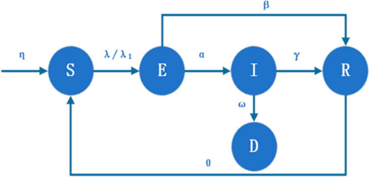
FIGURE 1. Diagram of the SEIRD model transmission mechanism.
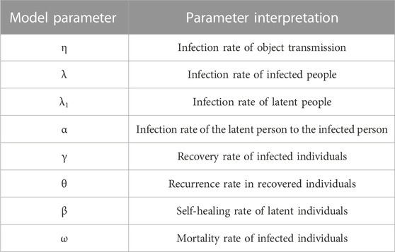
TABLE 1. Definition and interpretation of model parameters.
According to the system modeling idea, the relationship between different populations in the SEIRD model can be described by a system of differential equations. The total number of users is set to N and satisfies N(t) = S(t) + E(t) + I(t) + R(t) + D(t), and the system of equations for susceptible, exposed, infected, recovered, and dead people over time is as follows [22]:
The initial conditions are S(0) > 0, E(0) ≥ 0, I(0) > 0, R(0) ≥ 0, D(0) ≥ 0.
According to the actual background of the model, in order to analyze the stability of the model, the equilibrium point of the model should be considered in the bounded region. The equilibrium point is mainly the point with or without disease transmission and the local equilibrium point. When variables E and I are both 0 (there is no infected person or sleeper), we call such a point as the disease-free equilibrium point. To determine the disease-free equilibrium point, we can make the set of equations as 0, dS/dt = 0, dE/dt = 0, dI/dt = 0, and dR/dt = 0, in which we obtain the system of equation non-zero solutions, from which it follows that
Then, by calculation, the solution of the system of equations is the equilibrium point of S, E, I, and R. For the case of the disease-free equilibrium point E = I = 0, according to Equations 6–9, we can obtain
Then, the disease-free equilibrium point of the model is
However, the disease-free equilibrium is a disease-free state, which is not the case we are interested in the real world, so the internal equilibrium is not focused on in this article. When neither E nor I is 0 (i.e., there are infected persons and exposed persons), we use the local equilibrium point to represent the possibility of disease transmission, a relatively stable equilibrium point in the epidemic transmission. When S ≠ 0, E ≠ 0, I ≠ 0, R ≠ 0, we can obtain the solution of the internal equilibrium point through programming calculation, according to (6)–(9).
The Jacobi matrix is obtained according to Equations 1–4 [23]:
In turn, the eigenvalues of the Jacobi matrix in the equation can be found from the aforementioned equation as
Then, we substitute (10) and E = 0 and I = 0 into Eq. 14 to obtain
After simplifying, we can turn this equation into a polynomial. The polynomial on μ can be obtained after collation (see the appendix for details), with A denoting the coefficient of μ3, B denoting the coefficient of μ2, C denoting the coefficient of μ, and D denoting the algebraic equation without μ. Then, the equation can be transformed as follows:
Since the Cartesian sign rule can be used to determine the number of positive or negative roots of a polynomial, it follows from the Cartesian sign rule [24] that the number of negative roots of the characteristic equation is equal to the number of changes in the sign of the coefficients such that the equation satisfies the condition of Eq. 16 to have four negative values, i.e., μ1 < 0, μ2 < 0, μ3 < 0, μ4 < 0, and satisfy the conditions A > 0, B > 0, C > 0, and D > 0. The roots of the characteristic equations of the resulting model are all negative, so the model is globally convergent.
According to the research related to the infectious disease model, there exists a threshold value R0 in the transmission of infectious diseases, and this threshold is also called the basic regeneration number; when R0 ≤ 1, the transmission of infectious diseases will die out naturally with time; while R0 > 1, the infectious disease will break out within a certain period of time. Since the next-generation matrix method [25] is widely used in epidemiology and the calculation of the basic regeneration number, in dynamic populations, this paper mainly uses the next-generation matrix method to calculate R0. There are two compartments in the model proposed in this paper, namely, E(t) and I(t). According to Eqs 1–5, the vector of X can be obtained by applying the next-generation matrix method, and then, the expressions on F, V are written based on the obtained vectors as follows:
Finding the Jacobi matrix for F, V, we obtain
The SEIRD model corresponding to R0 is the maximum eigenvalue of FV−1:
Furthermore, according to the next-generation matrix method, we can obtain
Theorem 1: The system model in the system of Equations 1–4 is globally asymptotically stable if R0 ≤ 1. Theorem 2: If R0 > 1, then the system model in the system of Equations 1–4 is not globally asymptotically stable. Proof: First, we assume that δ is an eigenvector of the matrix F and that
Under the condition of V-1F = R0, we obtain
Let Lyapunov function [26] be
So,
Organize
Here, if R0 ≤ 1, then
If we substitute E = 0, then we can obtain
namely,
Then, it can further be obtained that when R0 ≤ 1, then
In order to get the experimental results closer to the real situation in the real world, at the same time, we can better observe the change trend and change quantity of each stage of the infection model. The simulation experiment [27] considers the number of people in a big city as the standard and sets the initial total population as N = 107. At the same time, considering the initial approximate number of each population, we set the initial population density as follows:
S(0) = 107 − 1, E(0) = 0, I(0) = 1, R(0) = 0, and D(0) = 0.
At the same time, through observation, we found that when E(t) = I(t) = 0, there is no infection case in the model, and we can assume that the model has reached a stable state at this time. Figure 2 is a simulation diagram of the SEIRD model, through which we can witness the relationship between the density of five types of individuals and time in the propagation process. It can be seen from the following figure that at the beginning of the epidemic spread, the number of each population has hardly changed, which is quite consistent with the difficulty in finding the epidemic at the beginning. In the middle period of the epidemic spread, that is, the sudden period of epidemic, the number of people began to change significantly. In a short period of time, the number of susceptible people rapidly decreased, while the number of the infiltrator and infected people increased sharply. Mapped to reality, the epidemic situation has attracted the attention of government departments and the general public at this time, and began to carry out epidemic prevention and control in a strategic and organized way. The outbreak period was ushered in a short time after the outbreak period, the number of infected people reached its peak, and then, death cases began to appear. Because effective treatment and safety measures have been considered this time, the number of infected people begins to decrease after reaching the peak, and the number of recovered people is gradually increasing. Because the model also considers that the recovered patients may be re-infected after a period of recovery, the number of recovered patients will decrease and the number of susceptible people will increase in the later period. At the same time, the number of infected people will approach 0, the number of dead people will no longer increase, and the model will reach a stable state.
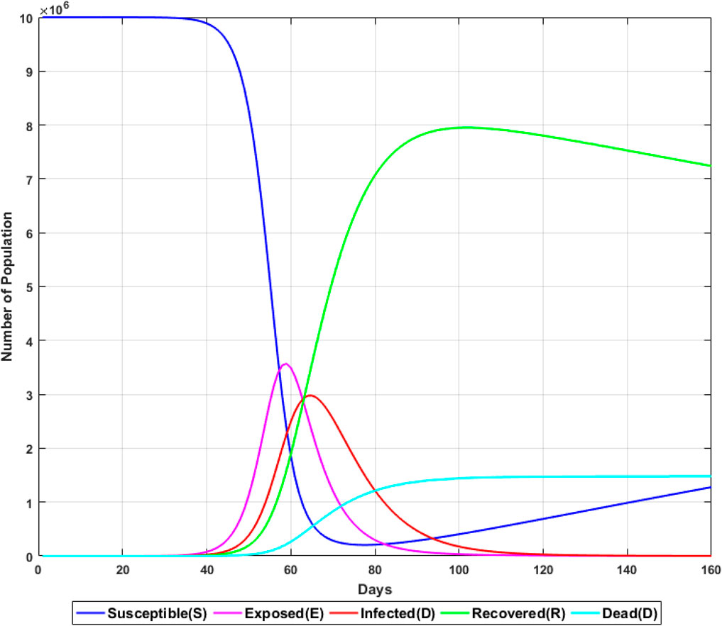
FIGURE 2. Simulation diagram of the SEIRD model simulation experiment.
In the real process of spreading the epidemic, each factor is very important for the final result. Therefore, in simulation training, some important parameters should be simulated with different values, such as cold chain transmission probability, infected person transmission probability, rehabilitation rate, and recovery rate, and the results of numerical simulation should be compared and analyzed to achieve better prediction results. In the spread of the epidemic, the number of the lurker and infected people is very important for the prevention and control of the epidemic, so in the simulation experiment, we focus on observing the changing trend of the lurker and infected persons so as to obtain an ideal prediction result of the epidemic.
Object transmission [28] mainly means that viruses can also spread to various people along with external media. At the beginning of the epidemic, people did not realize that the virus could spread in the cold chain. Later, after the local epidemic spread was blocked, many clustered epidemics occurred in various places. Finally, through investigation and study, novel coronavirus has strong viability on the surface of frozen products, and the continuous low temperature and humid cold chain environment also provide necessary conditions for the survival of novel coronavirus. Then, people began to pay attention to the prevention and control of object transmission. Figure 3 shows a simulation chart of the influence of object transmission probability η on epidemic transmission.
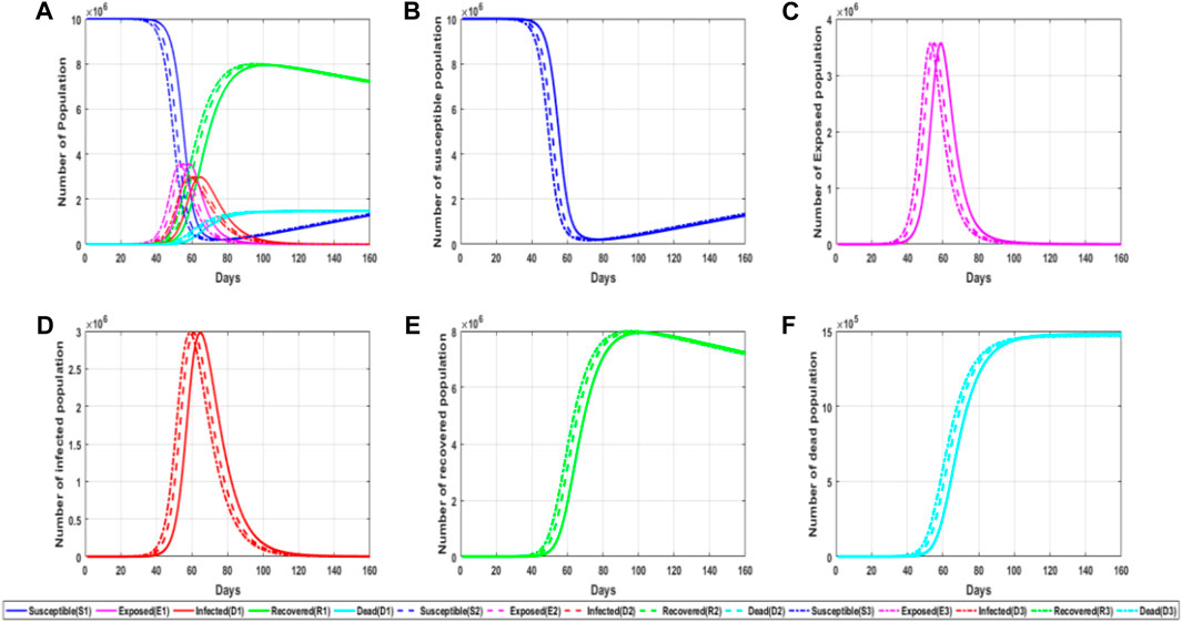
FIGURE 3. Simulation diagram of the influence of object propagation probability on the epidemic. (A) General map of simulated trends in different populations for different values of the parameters of object propagation; (B) trends in the number of susceptible persons for different parameter values of object propagation; (C) trends in the number of latent persons for different values of the parameters of object transmission; (D) trends in the number of infected persons for different values of the parameters of object transmission; and (E) trends in the number of recovered persons for the different values of the parameters of object transmission. (F) Trends in the number of fatalities for different values of object propagation parameters.
From the information observed in the figure, it can be found that different object transmission probability values will also have different impacts on the experiment. The greater the object transmission probability value, the faster the epidemic spread, and then the infiltrator and infected people will peak earlier, that is, enter the outbreak period faster. At the same time, we find that the increase in object propagation probability will lead to the peak appearing ahead of time, but it will not change the peak basically. It can be seen that reducing the spread of objects can help us slow down the spread of the epidemic. Usually, we strictly control overseas food and disinfect public places in order to reduce the spread probability of objects, thus slowing down the spread speed.
The virus infection rate is mainly divided into the infection rate of the infiltrator to the susceptible person and the infection rate of the infected person to the susceptible person. Figure 4 shows a simulation chart of the influence of the virus infection probability λ on the spread of the epidemic situation.
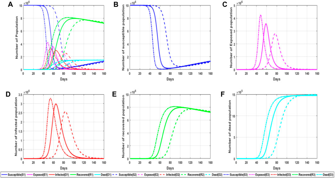
FIGURE 4. Simulation diagram of the influence of object propagation probability on the epidemic. (A) General graph of simulated trends in the probability of viral infection for different populations at different parameter values; (B) trends in the number of susceptible persons at different parameter values of the probability of viral infection; (C) trends in the number of latent persons at different parameter values of the probability of viral infection; (D) trends in the number of infected persons at different parameter values of the probability of viral infection; and (E) trends in the number of convalescent persons at different parameter values of the probability of viral infection. (F) Trends in the number of deaths for different values of the probability of viral infection parameter.
It can be seen from the aforementioned figure that the infection rate has a significant impact on the epidemic situation. The probability of virus infection can not only affect the peak time of the lurker and infected people but also affect their peak value. It can also be observed from the figure that the number of infected people increases rapidly when the number of the infiltrator reaches its peak, so the growth trend of infected people can be judged by the number of the infiltrator. We found that the greater the value of infection probability, the earlier the change of each population, and the infection rate has different degrees of influence on each population, including the number of recovered patients and susceptible people in the later stage of infection. On one hand, this also explains the importance of wearing a mask because wearing a mask can effectively reduce the probability of infection as it not only reduces the number of infected people but also delays the onset time of infected people and reduces the probability of infection, which is more conducive to our prevention and control of the epidemic.
In addition to the great influence of infection probability on the spread of the epidemic, the probability of contact with susceptible people in the infiltrator is also very important for the spread of the epidemic. Because the infected person is an individual who has been diagnosed and has taken relevant isolation measures, this person does not have the ability of contact and transmission for the time being, and the contact probability is mainly for the infiltrator. Figure 5 shows a simulation chart of the influence of contact probability in the infiltrator on the epidemic spread.
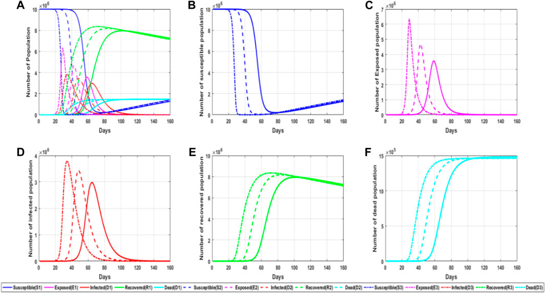
FIGURE 5. Simulation of the impact of sleeper contact probability on the epidemic. (A) General plot of simulated trends in the probability of latent exposure for different populations for different parameter values; (B) trends in the number of susceptible persons for different parameter values of the probability of latent exposure; (C) trends in the number of latent persons for different parameter values of the probability of latent exposure; (D) trends in the number of infected persons for different parameter values of the probability of latent exposure; and (E) trends in the number of convalescent persons for different parameter values of the probability of latent exposure. (F) trends in the number of deaths for different parameter values of the probability of latent exposure.
From the aforementioned figure, it can be found that the greater the contact probability, the greater the probability of infection to susceptible persons. This also explains why once more infected people are found, measures such as reducing travel and isolating at home are adopted because some symptoms of the infiltrator have not been found yet, but it may spread to other people, so it is necessary to reduce the contact probability at this time. The greater the contact probability, the higher the possibility that the susceptible person will be infected. At the same time, the faster and shorter the time required for the susceptible person to become the infiltrator, which will eventually lead to a higher peak value in the infiltrator, that is, the number of the infiltrator will greatly increase. The sharp increase in the number of infected people will bring great challenges to the prevention and control of the epidemic, so when the outbreak is serious, travel is generally restricted and contact is reduced.
Recovery probability is one of the most important factors in epidemic prevention and control. As long as the recovery probability is relatively high in the process of epidemic spread, the epidemic can end quicker, and the losses caused are relatively small. It can be seen that recovery probability is very important for us to study the spread of an epidemic. The recovery probability in this work means that the virus carrier does not carry the virus after treatment or autoimmunity and can no longer spread to others. The self-healing probability of the incubation period and the successful treatment probability of infectious patients belong to recovery probability. Figure 6 shows a simulation chart of the impact of recovery probability γ on the epidemic spread.
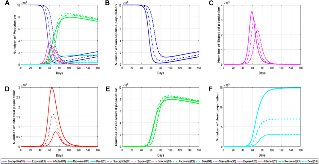
FIGURE 6. Simulation diagram of the influence of recovery probability on an epidemic situation. (A) General graph of simulated trends in the probability of recovery for different populations at different parameter values; (B) trends in the number of susceptible persons at different parameter values of the probability of recovery; (C) trends in the number of latent persons at different parameter values of the probability of recovery; (D) trends in the number of infected persons at different parameter values of the probability of recovery; and (E) trends in the number of recovered persons at different parameter values of the probability of recovery. (F) trends in the number of deaths at different parameter values of the probability of recovery.
As can be seen from the aforementioned figure, the higher the probability of recovery, the quicker the epidemic will end; the peak value of the infiltrator and infected people will decrease tremendously, and the time to reach the peak value will be delayed, and the number of dead people will also decrease significantly. Therefore, it can be concluded that under the condition of a relatively high recovery rate, all groups in the spread of the epidemic are developing toward a more ideal situation. From this figure, it can be concluded that constantly studying more effective therapeutic drugs and encouraging the general public to vaccinate are all aiming at improving the self-healing and healing abilities so that we can take more initiative in epidemic prevention and control.
The repositive rate [29] refers to the probability that patients are re-infected with viruses and become virus carriers after a period of recovery. In the early stage of the epidemic, the rate of recovery did not attract great attention. With the deepening of research and strict control, it was gradually found that the recovered patients still had the probability of becoming infected after a period of time. Figure 7 is a simulation chart of the influence of repositive probability θ on the epidemic spread.
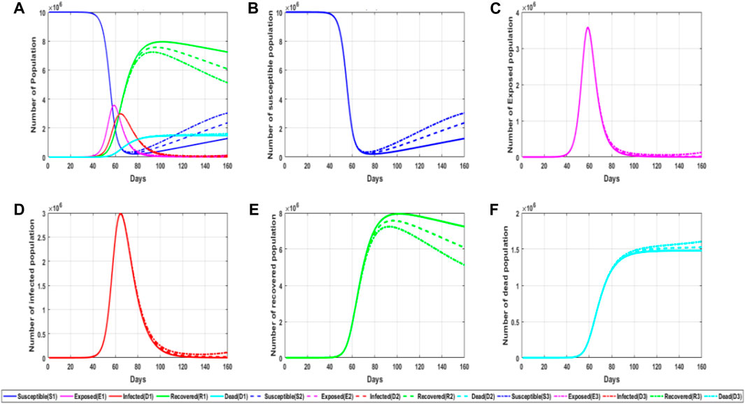
FIGURE 7. Simulation diagram of the influence of the probability of relapse on the epidemic. (A) General graphs of simulated trends in different populations for the different parameter values of the repositive probability; (B) trends in the number of susceptible persons for different parameter values of the repositive probability; (C) trends in the number of latent persons for different parameter values of the repositive probability; (D) trends in the number of infected persons for different parameter values of the repositive probability; and (E) trends in the number of recovered persons for different parameter values of the repositive probability. (F) Trends in the number of deaths for different values of the repositive probability parameter.
From the aforementioned figure, it can be concluded that in the early stage of the epidemic, the reactivation rate will not affect the number change of each population, but in the middle stage of the epidemic, with the increase in the number of recovered patients, the reactivation rate begins to affect the number change of the population. The higher the recovery rate, the number of recovered patients will gradually decrease, and the peak value of recovered patients will be advanced and reduced. For susceptible people, the number of this population will increase in the later period, but it can be seen that the repositive rate has little impact on the lurker and infected people and will only slightly increase the number of infected people in the later period, which also shows from the side that the repositive and the first-time infected people have almost the same impact in epidemic prevention and control. Therefore, mapped to the actual epidemic prevention, even if there are some antibodies in the recovered patients, they still carry out the same management as ordinary susceptible people in the epidemic control.
The genetic algorithm (GA) was first proposed by John Holland. It is an algorithm that helps find the optimal solution or approximate optimal solution to complex problems by simulating the process of natural evolution. The algorithm is designed according to the evolution of organisms in nature. Through mathematical methods and computer simulation operations, the algorithm converts the problem solving process into processes similar to the crossover and variation of chromosome genes in biological evolution. When solving more complex combinatorial optimization problems, compared with some conventional optimization algorithms, better optimization results can usually be obtained relatively quickly. At present, genetic algorithms have been widely used in various fields.
Compared with traditional optimization algorithms, the genetic algorithm uses probability rules instead of certain rules. Therefore, the genetic algorithm has the characteristics of global optimization and simple operation, which is suitable for solving complex optimization problems. In this work, the genetic algorithm is used to analyze the impact of different types of population on disease dynamics, optimize model parameters, and consider the changes of objective factors such as the gradual improvement of isolation measures in the early and late stages of the epidemic. Using the simulation software application MATLAB, an improved SEIRD epidemic prediction model was built. First, we consider that the incubation period is contagious and rehabilitative, and second, we consider that the recovered person is repositive and the infected person is fatal. Finally, the epidemiological transmission trends with different probability in different periods are simulated so that the prediction results are obtained.
In the face of complex non-linear optimization problems, the traditional genetic algorithm is prone to insufficient optimization ability, causing the algorithm to fall into a local optimal solution. In this article, an improved adaptive genetic algorithm (AGA) is used to change the heterogeneity and crossover rate through the adaptive adjustment of genetic parameters to achieve the retention of excellent individuals of offspring, which not only improves the convergence accuracy of genetic algorithms but also accelerates the convergence speed. In AGA, the cross probability Px and the variation probability Pm are adaptively adjusted according to the following:
In the formula, fmax represents the maximum adaptation value in the population, favg represents the average adaptation value of each generation of population, f′ represents the larger of the adaptation values of two individuals to cross, f represents the adaptation value of the individual to be mutated, and k1, k2, k3, and k4 consider the value of the (0,1) interval.
It can be seen from the formula that as the population evolves, the solution may be aggregated to the optimal solution, and favg gradually approaches fmax so that the cross-probability Px and the variation probability Pm gradually decrease, which helps maintain the excellent structure that the population has formed. In the same generation of populations, the probability of crossover and mutation of different individuals changes linearly with their own adaptation values. The lower the probability of crossover and variation in individuals with higher adaptability, the greater the probability of crossover and variation in individuals with lower adaptability. When the adaptive value of an individual is equal to the optimal adaptation value fmax in the contemporary population, its crossover and variation probabilities are calculated to be 0 by a formula, which allows these excellent individuals to be preserved, but it is likely that these excellent individuals will grow exponentially in the evolutionary process, resulting in an excessive convergence. In order to solve this problem, we choose to search for the global optimal solution by individuals with less than average adaptive values in the population.
1) Algorithm steps. Randomly select an initial group and represent each individual in the population with a string, and then evaluate the adaptation value of the randomly generated initial group, according to the adaptability function. If the optimal individual in the group does not improve for several consecutive generations, let the individual’s adaptability be the optimal adaptation value, and if the optimal adaptation value is not reached, it will enter the next round of evolution. When selecting the operation, select individuals from the population to inherit according to the optimal preservation strategy and the rules of roulette wheel selection, and pass on excellent individuals directly to the next generation or cross-generate new individuals through pairing and then to the next generation. In the crossover operation, choose two as parents in the population and randomly set an intersection point. The structure behind the point is interchangeable to generate two new individuals until the crossover stops after reaching the best. During the mutation operation, an individual in the population is randomly selected and the gene values on some locus in the individual chromosome coding string are replaced with other alleles of the locus until the mutation process stops after reaching the best value, forming a new individual. Calculate the adaptability function value of individuals in the new generation of population and replace the individuals with the worst adaptive individuals. If the best adaptation value is not reached, the improvement strategy will return to continue to evolve, and if the best adaptation value is reached, the best results will be output.
The main steps and flowchart of the genetic algorithm are shown in Figure 8 below:
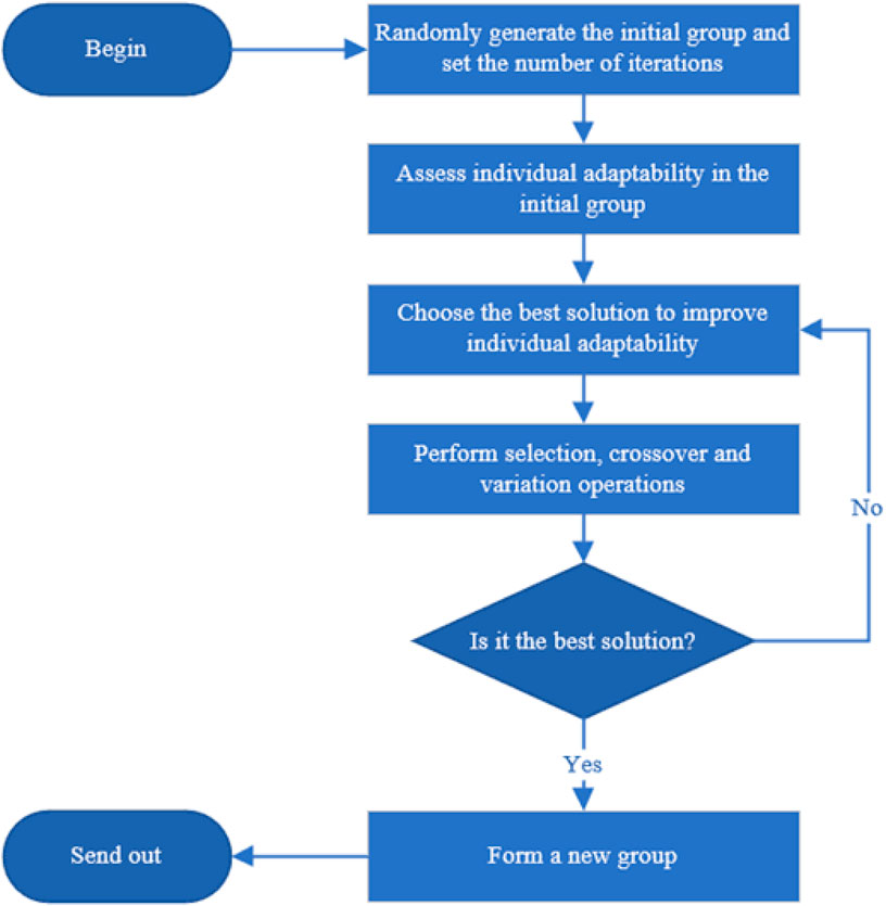
FIGURE 8. Algorithm step flowchart.
Input: M individuals, number of iterations t, and initial group P(t).
Output: New group P*(t).
1) Express the individual as a string, randomly generate the initial biological group P(t) comprising M individuals, and set the number of iterations t.
2) Assess the adaptability of each individual in the initial group.
3) Choose the best solution for improvement (selection, crossover, and variation).
4) Perform selection operations to inherit optimized individuals directly to the next generation or generate new individuals to the next generation by pairing intersections.
5) Perform cross-operations and act on the cross-operations on the group.
6) Carry out mutation operations and act on the mutation operator on the group. After selection, crossover, and mutation operations, group P(t) obtains the next-generation group P(t + 1).
7) Set the termination condition. If t = T, then use the individuals with maximum adaptability obtained during the evolutionary process as the optimal solution output to form a new group P*(t), and terminate the calculation.
2) Determination of adaptability function. In the evaluation of the adaptability function, in order to reflect the individual’s adaptability, it is necessary to introduce an adaptability function that can measure the individual’s adaptability. In the genetic algorithm for solving the parameters of the infectious disease model, the sum of the error square of the predicted and real values of the number of infected people infected in the infectious disease model is
3) Select the determination of the operator. The purpose of the selection is to inherit optimized individuals directly to the next generation or cross-generate new individuals through pairing and cross-generation so as to improve the global computing efficiency and adaptability. In this paper, a wide range of optimal storage strategies and roulette wheel selection are selected. The roulette gambling method selects a new population based on the probability proportional to the adaptability value (that is, the probability of each individual being selected is directly proportional to the value of its adaptability function). Each individual has the opportunity to be selected, which can improve the average adaptability value of the whole population without destroying the diversity of the population. However, this method is based on probability selection, with statistical errors. Sometimes even individuals with high adaptability are eliminated, and it is easy to converge to a local maximum. Another choice is the optimal preservation strategy, which sorts the individuals in the population according to the adaptability size, and then selects the most adaptive individuals to maintain them. This behavior can ensure that the optimal individual is not eliminated by random operations. However, because the selection of individuals is determined according to the sorting value, the optimization efficiency depends on the optimal individual.
The specific implementation step of the selection operator is a combination of roulette and optimal selection. Let the initial group size be n (even), and the adaptability function value of individual i is F(i). In the process of selecting individuals to inherit to the next generation, the idea of the optimal preservation strategy is adopted to sort individuals from high to low according to F(i), and the first n/2 individuals in the ranking are directly copied to the next-generation population. At the same time, the roulette selection method is used to select n/2 individuals from all individuals to inherit to the next generation so that the probability of individual i being selected to be inherited to the next-generation group is Pi = Fi/∑(
4) The selection of crossover and variability. When applying the genetic algorithm, the reasonable selection of the crossover rate and variability is an important factor affecting the efficiency of the algorithm. However, most genetic algorithms give an interval range when setting the crossover and mutation rates, of which the crossover rate is generally greater than 0.9 and between 0.9 and 0.99, and the mutation rate is relatively low, generally below 0.1, between 0.0001 and 0.1, but there is a lot of uncertainty and blindness in determining the approximate range of the cross rate and variability based on the empirical method.
In order to compare the influence of the application of the parameter optimization method of the adaptive genetic algorithm on the prediction accuracy of the propagation model, it is necessary to evaluate the prediction accuracy of the propagation model. In this paper, three indicators, namely, root mean square error (RMSE), average absolute error (MAE), and decision coefficient (R2), are used to evaluate the predictive accuracy of the model.
RMSE is another commonly used evaluation indicator, indicating that in the process of model fitting, it reflects the gap between the model prediction results and the actual results. The lower the RMSE, the more accurate the model is. However, it reflects an objective standard deviation. RMSE can be calculated according to the following formula:
MAE is another indicator used to evaluate the accuracy of model prediction results, which represents the gap between model prediction results and the actual results. MAE can be calculated by the following formula:
Among them, the value range of MAE is (0, +), which is equal to 0 when the predicted value exactly matches the real value, which is the perfect model; the greater the error, the greater the value.
The deciding coefficient (R2) indicates the fitting optimization of the regression model coefficient evaluated after linear regression. R2 reflects the proportion of all variations of model-dependent variables being interpreted by independent variables through the regression model. The larger the value of R2, the greater the variation in linear return model interpretation. R2 can be calculated according to the following formula:
When R2 is 1, it shows that there is no error between the prediction and the real observation values of the model, indicating that the interpretation of the independent variable to the dependent variable in the regression analysis is better; when R2 is 0, each prediction value of the sample in the model is equal to the mean; when R2 is close to 0, it indicates that the prediction ability of the model is poor, and the prediction effect is close to using the average of the observed value as the model prediction value. This means that the wrong model may have been used or the assumptions of the model are unreasonable.
By consulting the parameters of relevant case data in Wuhan, we set the number of people in close contact with normal people every day at p = 20. Because the infected person will have some symptoms, only half of the number of people are seen to be in close contact with normal people. In the process of simulation of the model by the adaptive genetic algorithm, the values of each parameter are set within a certain dynamic range, and then, the value of the model parameters is continuously optimized and improved through the algorithm to achieve the best prediction effect. The value of the model parameters is finally determined as follows:
η = 0.01, λ = 0.03, λ1 = 0.02, α = 0.14,
γ = 0.1, θ = 0.02, β = 0.005, and ω = 0.02.
At the same time, in order to verify the effectiveness of the method on the model, the text compares the actual data on the 2020 Wuhan epidemic [30] officially released by the China Health Commission with the trend based on the status of SEIRD nodes to further analyze the difference between the predicted and real values. Figure 9 shows a trend chart that shows the state of each node under real data based on the SEIRD model.
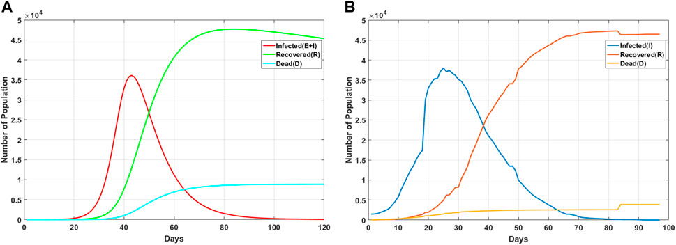
FIGURE 9. Change trend of nodes with different states over time. (A) Trend diagram of state nodes based on the SEIRD model. (B) Chart of epidemic trends in the real dataset.
From the figure, it can be seen that the data changes of the number of confirmed cases, and the number of recovered people and deaths in real situations are very similar to the trend of our prediction trend, so it can be shown that after the optimization of adaptive genetic algorithms, the SEIRD model can be applied to the spread of the real epidemic.
At the same time, it can be seen from the figure that the number of confirmed cases increased rapidly in the early stage, and the change trend was evident. However, with a series of measures, such as isolation and wearing masks, the number of confirmed cases gradually decreased, and the number of recovered cases gradually increased, and finally, the number of confirmed cases gradually returned to 0. The trend curve of the recovered patients is also in line with our prediction, and the number of recovered patients is gradually increasing, but in the end, due to the existence of the recovered patients, there will be a slight decline in the end. The trend of death tolls is basically consistent with our predicted results, which first increases slowly and finally tends to be stable. By comparing the actual data with the predicted data, it can be found that the SEIRD model can effectively simulate the spread trend of the actual epidemic situation and provide theoretical support for relevant departments.
The different types of infectious diseases each have different characteristics in transmission, and this paper is to establish a model to analyze from the perspective of the transmission mechanism. In order to verify the effect of this model in the transmission of new coronavirus causing pneumonia, this paper optimizes different models on the adaptive genetic algorithm and analyzes the data on the optimized classical model and this model, such as the SIR model, SEIR model, and the basic SEIRD model.
The SIR model is one of the most basic of infectious disease models, where S denotes susceptible, I denotes infected, and R denotes recovered. Transmission mechanism: at first, all nodes are in their susceptible state, some nodes reach the infected state after contacting the information, and the infected nodes infect other nodes or reach the recovered state. According to the system modeling idea, the relationship between different populations in the SIR model can be described by a system of differential equations. The total number of users is set as N and satisfies N(t) = S(t) + I(t) + R(t), and the system of equations of susceptible, infected, and recovered people over time is as follows:
The initial conditions are S(0) ≥ 0, I(0) > 0, R(0) ≥ 0.
The SEIR model is an improvement on the SIR model with the addition of the incubator E. Healthy people who have been in contact with a patient do not get sick immediately but become carriers of the pathogen. According to the system modeling idea, the relationship between different populations in the SEIR model can be described by a system of differential equations. The total number of users is set as N and satisfies N(t) = S(t) + E(t) + I(t) + R(t), and the system of equations for susceptible, exposed, infected, and recovered people over time is as follows:
The initial conditions are S(0) ≥ 0, E(0) ≥ 0, I(0) > 0, R(0) ≥ 0.
The basic SEIRD model is also improved on the basis of the SEIR model by adding the number of dead people, i.e., the number of people who died from the infection of the epidemic, and this model is more in line with the spread of the real epidemic. According to the system modeling idea, the relationship between different populations in the SEIRD model can be described by a system of differential equations. The total number of users is set as N and satisfies N(t) = S(t) + E(t) + I(t) + R(t) + D(t), and the system of equations for susceptible, exposed, infected, recovered, and dead people over time is as follows:
The initial conditions are S(0) ≥ 0, E(0) ≥ 0, I(0) > 0, R(0) ≥ 0, D(0) ≥ 0.
This model not only increases the number of dead people but also takes into account the object transmission, the re-positive rate of the recovered people, and the self-healing rate of the latent people, which is very close to the real transmission process of the new coronavirus causing pneumonia.
After the optimization of the adaptive genetic algorithm, the simulation trend of multiple models is shown in Figure 10.
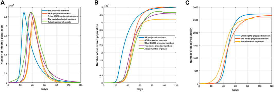
FIGURE 10. Comparative effect graphs of model simulations. (A) Trend graph of the number of infections predicted by the model simulation; (B) trend graph of the number of recoveries predicted by the model simulation; and (C) trend graph of the number of deaths predicted by the model simulation.
As can be seen in Figure 10A, the trend of infected persons predicted by each model is basically similar, the SIR model does not have an incubation period, and healthy people become infected immediately after contacting infected persons, so it causes the number of infected persons predicted by the SIR model to reach the peak in a relatively short period of time, which leads to the prediction results being very different from the actual infection data. The number of infected persons predicted by the SEIR model is very close to that of the real data, but the number of infected persons has a large gap compared with the real data, which is very close to the real data, but the number of infected people has a large gap compared with the real data, particularly because the SEIR model does not take into account the object transmission and repositive positivity rate, which leads to the actual number of infected people being more than predicted by the model. The underlying SEIRD model also does not take into account object transmission and the repositive positivity rate, and due to the death of some of the infected people, resulting in a lower number of predicted infected people compared to the real infected people. As can be seen from Figure 10B, there is a large difference in the number of recovered persons predicted by each model because the SIR and SEIR models do not take into account those who die, so the number of recovered persons predicted by the model is much higher than the actual number of recovered persons. The underlying SEIRD model also results in a lower number of recovered people than the real data due to the lower number of infected persons predicted by the model. Figure 10C shows that both the base SEIRD model and this model predict the number of deaths which are close to the real number of deaths but both are slightly higher in trend than the real death data; this is because the real data comprise the number of deaths after medical and drug interventions, which results in the predicted data to be higher than the real data. As can be seen in Figure 10, the improved model in this paper is more accurate in predicting the number of infections, recoveries, and deaths than other models, and is also more in line with the real data compared to the real data.
The mechanism of virus transmission is relatively complex in epidemic prevention and control, which requires a more accurate model. In this paper, a SEIRD epidemic transmission model is proposed, which includes factors such as object transmission, self-healing ability, recovery rate, and mortality. Based on this model, this work conducted simulation experiments on each influencing factor to analyze the impact of different factors on the spread of the epidemic. The experimental results show that although the cold chain input probability does not affect the final number of infected people, it will affect the time to reach the peak; the ability to heal is critical in determining the impact of infection, not only affecting the number of infected people but also accelerating the cycle of infection; although the recovery rate will not cause an increase in the number of infected people, it will affect the number of different groups in the later stage of the epidemic; mortality in epidemic prevention and control is closely related to the number of infected people. When the number of infected people is large and treatment is not timely, more deaths will occur. Finally, this work also improves and optimizes the model parameters through the adaptive genetic algorithm, simulates and analyzes the trend of the epidemic from many aspects, and compares and analyzes the real data. The results show that the model optimized by the algorithm can effectively predict the spread of the epidemic, and at the same time, it can bring certain theoretical reference values to epidemic prevention and control.
The original contributions presented in the study are included in the article/Supplementary Material; further inquiries can be directed to the corresponding author.
Methodology: SH and BC; validation: SH, BC, and XL; data curation: ZL, TC, and MJ; writing—original draft preparation: SH, TC, MJ, and BC; writing—review and editing: SH and BC. All authors contributed to the article and approved the submitted version.
This research was supported in part by the Humanities and Social Sciences Project of the Ministry of Education of China under grant no. 22YJCZH014, the National Natural Science Foundation of China under grant no. 61602202, the Natural Science Foundation of Jiangsu Province under contract no. BK20160428, and the Natural Science Foundation of Education Department of Jiangsu Province under contract no. 20KJA520008. Six talent peaks project in Jiangsu Province (grant no. XYDXX-034) and China Scholarship Council also supported this work. The author is grateful for the financial support provided by the aforementioned foundations.
The authors declare that the research was conducted in the absence of any commercial or financial relationships that could be construed as a potential conflict of interest.
All claims expressed in this article are solely those of the authors and do not necessarily represent those of their affiliated organizations, or those of the publisher, the editors, and the reviewers. Any product that may be evaluated in this article, or claim that may be made by its manufacturer, is not guaranteed or endorsed by the publisher.
The Supplementary Material for this article can be found online at: https://www.frontiersin.org/articles/10.3389/fphy.2023.1195087/full#supplementary-material
1. Zisad SN, Hossain MS, Hossain MS, Andersson K. An integrated neural network and seir model to predict covid-19. Algorithms (2021) 14:94. doi:10.3390/a14030094
2. Lacitignola D, Diele F. Using awareness to z-control a seir model with overexposure: Insights on covid-19 pandemic. Chaos, Solitons & Fractals (2021) 150:111063. doi:10.1016/j.chaos.2021.111063
3. Verma T, Gupta AK. Network synchronization, stability and rhythmic processes in a diffusive mean-field coupled seir model. Commun Nonlinear Sci Numer Simulation (2021) 102:105927. doi:10.1016/j.cnsns.2021.105927
4. Yuan X, Chen S, Yuwen L, An S, Mei S, Chen T. An improved seir model for reconstructing the dynamic transmission of covid-19. In: Proceedings of the 2020 IEEE International Conference on Bioinformatics and Biomedicine (BIBM); December 2020; Seoul, Korea (South). IEEE (2020). p. 2320–7.
5. Husein I, Mawengkang H, Suwilo S, Mardiningsih S. Modeling the transmission of infectious disease in a dynamic network. J Phys Conf Ser (2019) 1255:012052. doi:10.1088/1742-6596/1255/1/012052
6. Simha Au., Prasad RV, Narayana S. A simple stochastic sir model for covid 19 infection dynamics for Karnataka: Learning from europe (2020). Available at: https://arxiv.org/abs/2003.11920.
7. Cooper I, Mondal A, Antonopoulos CG. A sir model assumption for the spread of covid-19 in different communities. Chaos, Solitons & Fractals (2020) 139:110057. doi:10.1016/j.chaos.2020.110057
8. Gaeta G. A simple sir model with a large set of asymptomatic infectives (2020). Available at: https://arxiv.org/abs/2003.08720.
9. Zakary O, Rachik M, Elmouki I. On the analysis of a multi-regions discrete sir epidemic model: An optimal control approach. Int J Dyn Control (2017) 5:917–30. doi:10.1007/s40435-016-0233-2
10. Harko T, Lobo FS, Mak M. Exact analytical solutions of the susceptible-infected-recovered (sir) epidemic model and of the sir model with equal death and birth rates. Appl Math Comput (2014) 236:184–94. doi:10.1016/j.amc.2014.03.030
11. Shan C, Zhu H. Bifurcations and complex dynamics of an sir model with the impact of the number of hospital beds. J Differential Equations (2014) 257:1662–88. doi:10.1016/j.jde.2014.05.030
12. Zhang J-Z, Jin Z, Liu Q-X, Zhang Z-Y. Analysis of a delayed sir model with nonlinear incidence rate. Discrete Dyn Nat Soc (2008) 2008:1–16. doi:10.1155/2008/636153
13. Abdy M, Side S, Annas S, Nur W, Sanusi W. An sir epidemic model for covid-19 spread with fuzzy parameter: The case of Indonesia. Adv difference equations (2021) 2021:105–17. doi:10.1186/s13662-021-03263-6
15. Mwalili S, Kimathi M, Ojiambo V, Gathungu D, Mbogo R. Seir model for covid-19 dynamics incorporating the environment and social distancing. BMC Res Notes (2020) 13:352–5. doi:10.1186/s13104-020-05192-1
16. He S, Peng Y, Sun K. Seir modeling of the covid-19 and its dynamics. Nonlinear Dyn (2020) 101:1667–80. doi:10.1007/s11071-020-05743-y
17. Artalejo JR, Economou A, Lopez-Herrero MJ. The stochastic seir model before extinction: Computational approaches. Appl Math Comput (2015) 265:1026–43. doi:10.1016/j.amc.2015.05.141
18. Kamrujjaman M, Ghosh U, Islam MS. Pandemic and the dynamics of seir model: Case covid-19 (2020).
19. Li J, Cui N. Dynamic analysis of an seir model with distinct incidence for exposed and infectives. Scientific World J (2013) 2013:1–5. doi:10.1155/2013/871393
20. Syafruddin S, Noorani MSM. Lyapunov function of sir and seir model for transmission of dengue fever disease. Int J Simul Process Model (2013) 8:177–84. doi:10.1504/ijspm.2013.057544
21. Liu F, Wang J, Liu J, Li Y, Liu D, Tong J, et al. Predicting and analyzing the covid-19 epidemic in China: Based on seird, lstm and gwr models. PloS one (2020) 15:e0238280. doi:10.1371/journal.pone.0238280
22. Piccolomini EL, Zama F. Preliminary analysis of covid-19 spread in Italy with an adaptive seird model (2020). Available at: https://arxiv.org/abs/2003.09909.
23. Youssef HM, Alghamdi NA, Ezzat MA, El-Bary AA, Shawky AM. A new dynamical modeling seir with global analysis applied to the real data of spreading covid-19 in Saudi Arabia. Math Biosci Eng (2020) 17:7018–44. doi:10.3934/mbe.2020362
24. Mammeri Y. A reaction-diffusion system to better comprehend the unlockdown: Application of seir-type model with diffusion to the spatial spread of covid-19 in France. Comput Math Biophys (2020) 8:102–13. doi:10.1515/cmb-2020-0104
25. Intissar A. A mathematical study of a generalized seir model of covid-19. SciMedicine J (2020) 2:30–67. doi:10.28991/scimedj-2020-02-si-4
26. Korobeinikov A. Lyapunov functions and global properties for seir and seis epidemic models. Math Med Biol a J IMA (2004) 21:75–83. doi:10.1093/imammb/21.2.75
27. Younsi F-Z, Bounnekar A, Hamdadou D, Boussaid O. Seir-sw, simulation model of influenza spread based on the small world network. Tsinghua Sci Tech (2015) 20:460–73. doi:10.1109/tst.2015.7297745
28. Yang F, Zhang Z. A time-delay covid-19 propagation model considering supply chain transmission and hierarchical quarantine rate. Adv Difference Equations (2021) 2021:191–21. doi:10.1186/s13662-021-03342-8
29. Zhou X, Cui J. Analysis of stability and bifurcation for an seir epidemic model with saturated recovery rate. Commun nonlinear Sci Numer simulation (2011) 16:4438–50. doi:10.1016/j.cnsns.2011.03.026
Keywords: epidemic transmission, self-healing rate, lethality, repositive rate, adaptive genetic algorithm
Citation: Chen B, Han S, Liu X, Li Z, Chen T and Ji M (2023) Prediction of an epidemic spread based on the adaptive genetic algorithm. Front. Phys. 11:1195087. doi: 10.3389/fphy.2023.1195087
Received: 28 March 2023; Accepted: 20 September 2023;
Published: 04 October 2023.
Edited by:
Guillermo Huerta Cuellar, University of Guadalajara, MexicoReviewed by:
Junchan Zhao, Hunan University of Technology and Business, ChinaCopyright © 2023 Chen, Han, Liu, Li, Chen and Ji. This is an open-access article distributed under the terms of the Creative Commons Attribution License (CC BY). The use, distribution or reproduction in other forums is permitted, provided the original author(s) and the copyright owner(s) are credited and that the original publication in this journal is cited, in accordance with accepted academic practice. No use, distribution or reproduction is permitted which does not comply with these terms.
*Correspondence: Shuai Han, aGFuc2h1YWk2MjYyQGdtYWlsLmNvbQ==
Disclaimer: All claims expressed in this article are solely those of the authors and do not necessarily represent those of their affiliated organizations, or those of the publisher, the editors and the reviewers. Any product that may be evaluated in this article or claim that may be made by its manufacturer is not guaranteed or endorsed by the publisher.
Research integrity at Frontiers
Learn more about the work of our research integrity team to safeguard the quality of each article we publish.