Efficient modeling of sharp-edge acoustofluidics

Sharp-edge structures exposed to acoustic fields are known to produce a strong non-linear response, mainly in the form of acoustic streaming and acoustic radiation force. The two phenomena are useful for various processes at the microscale, such as fluid mixing, pumping, or trapping of microparticles and biological cells. Numerical simulations are essential in order to improve the performance of sharp-edge-based devices. However, simulation of sharp-edge structures in the scope of whole acoustofluidic devices is challenging due to the thin viscous boundary layer that needs to be resolved. Existing efficient modeling techniques that substitute the need for discretization of the thin viscous boundary layer through analytically derived limiting velocity fail due to large curvatures of sharp edges. Here, we combine the Fully Viscous modeling approach that accurately resolves the viscous boundary layer near sharp edges with an existing efficient modeling method in the rest of a device. We validate our Hybrid method on several 2D configurations, revealing its potential to significantly reduce the required degrees of freedom compared to using the Fully Viscous approach for the whole system, while retaining the relevant physics. Furthermore, we demonstrate the ability of the presented modeling approach to model high-frequency 3D acoustofluidic devices featuring sharp edges, which will hopefully facilitate a new generation of sharp-edge-based acoustofluidic devices.

1 Introduction

Acoustofluidic devices commonly exploit two phenomena, namely, acoustic streaming (AS) and acoustic radiation force (ARF), for an increasing variety of tasks due to their ability to precisely manipulate fluids and objects on the microscale and in a contactless manner [1]. A particular type of acoustofluidic device features sharp-edge structures inside an acoustically excited device. In such a configuration, sharp edges produce a strong response in the form of AS [2–5] and ARF [6, 7], as illustrated in Figure 1. The literature indicates that in most 2D cases, the AS around a single sharp edge manifests itself in the form of two counter rotating vortices, one on each side of the tip of the sharp edge, with the flow above the apex directed away from the edge tip [4]. As for the ARF, it has been shown that “heavy” microparticles get attracted to the excited sharp edge, whereas “light” particles get repelled from the edge [7].

FIGURE 1

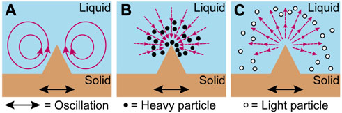
FIGURE 1. Illustration of the main phenomena driven by the oscillations of a sharp edge relative to the surrounding fluid: (A) the sharp-edge-driven acoustic streaming [4], (B) the attraction of “heavy” particles to the tip of the sharp edge due to the ARF [7], and (C) the ARF-based repulsion of “light” particles by the sharp edge [7].

Acoustically excited sharp edges can be used for micropumping [8, 9], trapping of biological cells [6, 10, 11], and powerful mixing [12–14]. Numerical models capable of predicting the behavior inside such devices and, thus, their performance are a valuable tool for design optimization. Especially, since the production of most acoustofluidic devices requires a cleanroom environment, making prototyping laborious and expensive. Furthermore, numerical simulations can give deeper insight into the underlying physics [2, 4, 5].

The modeling of harmonic acoustic fields at the scale of a typical acoustofluidic device for micromanipulation requires the modeling of one-half to several acoustic wavelengths λ = c₀/f, with the speed of sound in the fluid c₀ and the driving frequency f. Each wavelength is normally discretized with several tens of elements, making such a device possible to simulate as a whole 3D multiphysics problem. However, when analyzing higher-order steady phenomena in viscous fluids, such as AS, another characteristic length needs to be discretized-the viscous boundary layer thickness $\delta =\sqrt{\eta /(\pi {\rho }_{0}f)}$, with the dynamic fluid viscosity η and the density of the fluid ρ₀. In a typical acoustofluidic device, filled with water and driven at f = 1 MHz, we have λ ≈ 1.5 mm and δ = 0.56 µm. This indicates a large separation of length scales, with the device being $\mathcal{O}(\lambda )$, whereas the discretization at boundaries is required to resolve $\mathcal{O}(\delta )$. Muller et al. [15] introduced a Fully Viscous modeling approach based on the perturbation theory that resolves both λ and δ, requiring significant computational effort and is, thus, in most cases limited to simplified 2D models. Over the years, alternative approaches were developed that analytically solve AS in the viscous boundary layer and use the solution as a boundary condition for the flow in the fluid bulk. This so-called limiting velocity method (LVM) was already used in [16], [17, 18], [19], [20, 21], and others. Recently, [22] and [23] improved the LVM by accounting for the Stokes drift and thermal boundary layer, respectively. The LVM approach has already enabled 3D simulations of AS in a whole acoustofluidic device [19, 21, 24]. There is, however, a general limitation of the LVM, in which the radius of the curvature of boundaries in the system needs to be much larger than δ. This makes LVM as such unusable for the simulation of AS in acoustofluidic devices featuring sharp edges, since the behavior in such devices is greatly influenced by the behavior near the tips of sharp edges [5].

Sharp-edge acoustofluidics has been successfully modeled in several studies using the Fully Viscous approach, but typically in 2D [4, 13, 25, 26] and under further simplifications, such as assuming a periodicity across the device [3], using systems at low frequencies with the acoustic wavelength larger than the system (subwavelength system) [2, 5, 27], or exploiting symmetries [28]. Under these simplified conditions, a few studies featured the direct numerical simulations that revealed the threshold amplitude of the oscillatory excitation velocity at which the perturbation-based computation of the acoustic streaming near a sharp edge fails [2, 5, 29].

Here, we introduce a Hybrid modeling approach that fully resolves the viscous boundary layers in the vicinity of sharp edges, analogous to the approach of [15], while the rest of the acoustofluidic device is modeled using LVM-based approach derived by [22]. First, we validate the Hybrid approach against the Fully Viscous approach on a simple single-sharp-edge geometry, which is used in several previous studies [4, 5, 26]. Second, we apply the Hybrid approach to model a more complex acoustofluidic device that features a pair of sharp edges and is capable of pumping, as introduced recently in [9]. At last, we apply the Hybrid approach to model high-frequency sharp-edge acoustofluidics in 3D. The developed approach, depending on the complexity of the device, significantly decreases the required degrees of freedom (DOF) in the model compared to fully resolving the viscous boundary layer.

2 Methodology

In the current work, we model only the behavior of fluids within microfluidic channels, whereas the solids typically bounding such channels are replaced by suitable boundary conditions.

We assume a viscous fluid, the motion of which can be described by the compressible Navier–Stokes equations

$\begin{array}{ll}\hfill \rho \left[\frac{\partial \mathit{v}}{\partial t}+\left(\mathit{v}\cdot \mathbf{\nabla }\right)\mathit{v}\right]& =-\mathbf{\nabla }p+\eta {\nabla }^2\mathit{v}+\left({\eta }_{\mathrm{B}}+\frac{\eta }{3}\right)\mathbf{\nabla }\left(\mathbf{\nabla }\cdot \mathit{v}\right),\hfill \end{array}(1)$

and the continuity equation

$\frac{\partial \rho }{\partial t}=-\mathbf{\nabla }\cdot \left(\rho \mathit{v}\right),(2)$

with the velocity v, the dynamic viscosity η, and the bulk viscosity η_B. The fluid is assumed to be barotropic, and the density ρ, therefore, depends only on the pressure p, namely,

$\rho =\rho \left(p\right).(3)$

The equations are linearized using the regular perturbation approach [30]. Accordingly, the physical fields are expanded in a series □ = □₀ + □₁ + □₂ + …, where □ represents the field and the subscript denotes the respective order. The amplitude of the first-order velocity v₁ is, therefore, assumed to be small with respect to the speed of sound c₀—small Mach number assumption.

2.1 First-order (acoustic) problem

For a fluid quiescent at the zeroth order (v₀ = 0), the substitution of the first-order perturbed fields into governing Eqs. 1, 2 yields the set of first-order equations

${\rho }_0\frac{\partial {\mathit{v}}_1}{\partial t}=-\mathbf{\nabla }{p}_1+\eta {\nabla }^2{\mathit{v}}_1+\left({\eta }_{\mathrm{B}}+\frac{\eta }{3}\right)\mathbf{\nabla }\left(\mathbf{\nabla }\cdot {\mathit{v}}_1\right),(4)$

$\frac{\partial {\rho }_1}{\partial t}=-{\rho }_0\mathbf{\nabla }\cdot {\mathit{v}}_1,(5)$

with the equilibrium density ρ₀. The equation of state, namely Eq. 3, translates to

${\rho }_1=\frac{1}{c_0^2}{p}_1(6)$

and connects the first-order density with the first-order pressure. The first-order fields are assumed to have a harmonic time dependency through the factor e^iωt, with the angular frequency ω = 2πf and the imaginary unit i.

2.2 Second-order (streaming) problem

Applying the perturbation theory to the governing equations up to second order and taking the time average $⟨\square ⟩=\frac{1}{T}{\int }_T\square \mathrm{d}t$ over an oscillation period T lead to the equations of acoustic streaming [31]

$\mathbf{\nabla }⟨p_2⟩-\eta {\nabla }^2⟨{\mathit{v}}_2⟩=-{\rho }_0\mathbf{\nabla }\cdot ⟨{\mathit{v}}_1{\mathit{v}}_1⟩,(7)$

$\mathbf{\nabla }\cdot ⟨{\mathit{v}}_2⟩=0.(8)$

The time average of a product of first-order fields ${\square }_1={\tilde{\square }}_1{\mathrm{e}}^{\mathrm{i}\omega t}$, with the spatially-dependent and time-independent complex amplitude ${\tilde{\square }}_1$, is computed as $⟨{\square }_1{■}_1⟩=\frac{1}{2}\mathrm{R}\mathrm{e}\left[{\tilde{\square }}_1{\widetilde{■}}_1^{*}\right]$ with □* denoting a complex conjugate of □ [32]. For $⟨{\mathit{v}}_1{\mathit{v}}_1⟩$ in Eq. 7, the tensor product is implied. In Eqs 7, 8, the streaming field is considered to be incompressible, which is in line with related studies [33–36].

At the second order, the no-slip boundary condition is imposed on the Lagrangian velocity of the fluid at the fluid boundary. The Lagrangian velocity is defined as the sum of the Eulerian streaming velocity $⟨{\mathit{v}}_2⟩$ and the Stokes drift [37, 38]

${\mathit{v}}_{\mathrm{SD}}=⟨\left(\int {\mathit{v}}_1\mathrm{d}t\cdot \mathbf{\nabla }\right){\mathit{v}}_1⟩,(9)$

leading to the boundary condition on the Eulerian streaming velocity

$⟨{\mathit{v}}_2⟩=-{\mathit{v}}_{\mathrm{SD}}\text{at\hspace{0.17em}the\hspace{0.17em}boundary}.(10)$

For rigid boundaries that we assume in this work, v_SD reduces to zero.

This theoretical framework is only applicable as long as the perturbation theory is valid and as long as the streaming remains laminar. The validity of the perturbation theory approach in the context of sharp-edge streaming is further discussed in [2], [5].

2.3 Limiting velocity method

To compute the acoustic streaming one needs to solve the first- and the second-order problems outlined in the previous sections. Based on the complexity of the formulation, analytical solutions are rare and rely on basic geometries, simplified boundary conditions, and various assumptions regarding the relevant characteristic lengths, as, for example, performed in [16], [39], [34], [40]. However, under additional assumptions, the so-called limiting velocity method has been developed by [18], [38], [22], wherein the aforementioned equations are solved separately in the vicinity of boundaries, where the viscous boundary layer develops. The main assumption of the LVM is the smallness of the viscous boundary layer thickness δ relative to the acoustic wavelength λ = c₀/f and relative to the curvature R of the boundary surface. Additionally, the displacement of a moving boundary surface tangential to the boundary surface needs to be small relative to R, while the displacement normal to the boundary surface needs to be small relative to δ. The derivation of the fields in the boundary layer assumes a solenoidal first-order velocity field, and the resulting (limiting) streaming velocity is then applied to a simplified streaming problem originating from Eqs 7, 8 as a slip velocity at certain small distance from the boundary [18] or at the boundary itself [22], depending on the formulation. It is important to note that the derivations in [22] are developed for e^−iωt time dependence, whereas the interfaces of the Acoustics Module of COMSOL Multiphysics that we use for implementation assume e^iωt. In the continuation, the formulation from [22] is, therefore, adapted to the COMSOL Multiphysics-compatible e^iωt.

The first-order problem, in the scope of the LVM, is simplified by assuming that the velocity field in the fluid bulk is irrotational, which leads to the Helmholtz equation

${\nabla }^2{p}_1+k_{\mathrm{c}}^2{p}_1=0,(11)$

with p₁ as the only unknown variable and with the viscous compressional wavenumber

$k_{\mathrm{c}}=\left(1-\mathrm{i}\frac{\mathrm{\Gamma }}{2}\right)\frac{\omega }{c_0},(12)$

with the damping coefficient

$\mathrm{\Gamma }=\left({\eta }_{\mathrm{B}}+\frac{4}{3}\eta \right)\frac{\omega }{{\rho }_0{c}_0^2}.(13)$

The first-order velocity is separated as

${\mathit{v}}_1={\mathit{v}}_1^{\mathrm{b}}+{\mathit{v}}_1^{\delta },(14)$

into a sum of the irrotational (∇ ×□ = 0) long-range velocity in the bulk of the fluid ${\mathit{v}}_1^{\mathrm{b}}$ and the solenoidal (∇ ⋅□ = 0) short-range velocity in the viscous boundary layer ${\mathit{v}}_1^{\delta }$. The velocity in the bulk is connected to the pressure through

${\mathit{v}}_1^{\mathrm{b}}=\frac{\mathrm{i}-\mathrm{\Gamma }}{\omega {\rho }_0}\mathbf{\nabla }{p}_1.(15)$

To account for the damping of the viscous boundary layer, the following condition needs to be applied at the boundary:

$\begin{array}{ll}\hfill \mathit{n}\cdot \mathbf{\nabla }{p}_1& =\frac{\omega {\rho }_0}{\mathrm{i}-\mathrm{\Gamma }}\left[\mathit{n}\cdot {\mathit{V}}_1^0-\frac{\mathrm{i}}{k_{\mathrm{s}}}\mathbf{\nabla }\cdot {\mathit{V}}_1^0\right]\hfill \\ \hfill & -\frac{\mathrm{i}}{k_{\mathrm{s}}}\left[\frac{{\omega }^2}{c_0^2\left(1+\mathrm{i}\mathrm{\Gamma }\right)}{p}_1+{\left(\mathit{n}\cdot \mathbf{\nabla }\right)}^2{p}_1\right],\hfill \end{array}(16)$

with the outward pointing normal of the unit length n, the velocity of the harmonic boundary ${\mathit{V}}_1^0$, and the shear wavenumber

$k_{\mathrm{s}}=\frac{1-\mathrm{i}}{\delta }.(17)$

The second-order problem for the streaming in the bulk of the fluid is in LVM governed by

$\mathbf{\nabla }\cdot {\mathit{v}}_2^{\mathrm{b}}=0,(18)$

$\mathbf{\nabla }⟨p_2^{\mathrm{b}}⟩-\eta {\nabla }^2⟨{\mathit{v}}_2^{\mathrm{b}}⟩=\mathbf{\nabla }⟨{\mathcal{L}}_{\text{ac}}^{\mathrm{b}}⟩+\frac{\mathrm{\Gamma }\omega }{c_0^2}⟨{\mathit{S}}_{\text{ac}}^{\mathrm{b}}⟩,(19)$

with the bulk Lagrangian density

$⟨{\mathcal{L}}_{\text{ac}}^{\mathrm{b}}⟩=\frac{1}{2}\frac{1}{{\rho }_0{c}_0^2}⟨p_1^2⟩-\frac{1}{2}{\rho }_0⟨{\mathit{v}}_1^{\mathrm{b}}⟩(20)$

and the energy-flux density

$⟨{\mathit{S}}_{\text{ac}}^{\mathrm{b}}⟩=⟨p_1{\mathit{v}}_1^{\mathrm{b}}⟩.(21)$

The boundary condition that constrains the second-order problem is given in a form of a slip velocity

${\mathit{v}}_2^{\mathrm{b}0}=\left(\mathit{A}\cdot {\mathit{t}}_1\right){\mathit{t}}_1+\left(\mathit{A}\cdot {\mathit{t}}_2\right){\mathit{t}}_2+\left(\mathit{B}\cdot \mathit{n}\right)\mathit{n},(22)$

with orthogonal unit vectors t₁ and t₂ that are tangential to the boundary surface and with

$\begin{array}{ll}\hfill \mathit{A}& =-\frac{1}{2\omega }\mathrm{R}\mathrm{e}\left\{{\mathit{v}}_1^{\delta 0\ast }\cdot \mathbf{\nabla }\left(\frac{1}{2}{\mathit{v}}_1^{\delta 0}-\mathrm{i}{\mathit{V}}_1^0\right)\right.\hfill \\ \hfill & +\mathrm{i}{\mathit{V}}_1^{0\ast }\cdot \mathbf{\nabla }{\mathit{v}}_1^{\mathrm{b}}+\left[\frac{2-\mathrm{i}}{2}\mathbf{\nabla }\cdot {\mathit{v}}_1^{\delta 0\ast }\right.\hfill \\ \hfill & \left.\left.+\mathrm{i}\left(\mathbf{\nabla }\cdot {\mathit{V}}_1^{0\ast }-\left(\mathit{n}\cdot \mathbf{\nabla }\right)v_{1n}^{\mathrm{b}\ast }\right)\right]{\mathit{v}}_1^{\delta 0}\right\},\hfill \end{array}(23)$

$\mathit{B}=\frac{1}{2\omega }\mathrm{R}\mathrm{e}\left\{\mathrm{i}{\mathit{v}}_1^{\mathrm{b}0\ast }\cdot \mathbf{\nabla }{\mathit{v}}_1^{\mathrm{b}}\right\},(24)$

with $v_{1n}^{\mathrm{b}\ast }=\mathit{n}\cdot {\mathit{v}}_{1n}^{\mathrm{b}\ast }$; ${\mathit{v}}_1^{\delta 0}$ follows from the no-slip boundary condition at the first order as

${\mathit{v}}_1^{\delta 0}={\mathit{V}}_1^0-{\mathit{v}}_1^{\mathrm{b}0}.(25)$

The superscript □⁰ indicates that □ is evaluated at the boundary.

2.4 Numerical model

The numerical models implementing the first- and the second-order problems are developed in the finite-element method framework of COMSOL Multiphysics 5.6 [41]. In the analysis that follows, we use three kinds of numerical models, namely, (I) the Fully Viscous model that numerically solves Eqs. 4–8, 10 in line with the approach introduced in [15] and used in many studies since [5, 9, 28, 42], (II) the Full Limiting Velocity Method (FLVM) model that is based on the LVM of [22] and incorporates Eqs. 11, 16, 18, 19, and 22, and (III) the Hybrid model that uses the formulation of the Fully Viscous model in the vicinity of sharp edges and the LVM formulation in the rest of the fluid domain, as illustrated in Figure 2.

FIGURE 2

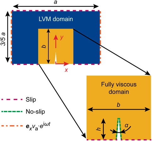
FIGURE 2. Geometry of the Hybrid model of a single sharp edge in a rectangular channel. The model is divided into a Fully Viscous domain (yellow) and a limiting velocity method domain (dark blue). The boundary conditions of the first-order problem are graphically indicated. The system is excited by an oscillatory velocity boundary condition along the x-axis, at x =±a/2 (dash-dotted line) with the velocity amplitude v_a. All walls of the LVM domain, including the driving wall, have an additional artificial velocity imposed according to [22] that accounts for damping inside the viscous boundary layer δ. The sharp edge in the Fully Viscous domain is modeled using the no-slip boundary condition, while the walls at the bottom of the edge are constrained with a slip boundary condition to improve the fully viscous-LVM interface. The geometric parameters describing the model are the channel width a, the Fully Viscous domain width b, the sharp-edge tip height h, the apex angle of the sharp edge α, and the radius of the rounding of the sharp-edge tip that is defined as δ/2, unless specified otherwise.

2.4.1 Fully viscous model

The Fully Viscous model is implemented in COMSOL Multiphysics by using the adiabatic form of the Thermoviscous Acoustics interface for the first-order problem, which is then solved with a Frequency Domain study. The second-order problem is implemented using the Creeping Flow interface, with the streaming source term $-{\rho }_0\mathbf{\nabla }\cdot ⟨{\mathit{v}}_1{\mathit{v}}_1⟩$ from Eq. 7, which is the spatial variation of the Reynolds stress, and added to the governing equations of the Creeping Flow interface as a volume force. The second-order problem is solved with the Stationary study.

The boundary conditions in the Fully Viscous model at the first order are the no-slip condition applied on all the non-moving (rigid) walls; specifically,

${\mathit{v}}_1=\mathbf{0}\text{at\hspace{0.17em}the\hspace{0.17em}non}-\text{moving\hspace{0.17em}walls},(26)$

while at the moving walls, the applied wall velocity is imposed as

${\mathit{v}}_1={\mathit{v}}_{\text{wall}}\text{at\hspace{0.17em}the\hspace{0.17em}moving\hspace{0.17em}walls},(27)$

with the velocity v_wall defined on the case-by-case basis. At the second order, the no-slip boundary condition is applied to all the walls, but on the Lagrangian velocity, as in Eq. 10. However, the Stokes drift that appears in Eq. 10 only at the moving walls.

2.4.2 Full Limiting Velocity Method model

The first-order problem of the FLVM model is implemented through the Pressure Acoustics interface, with the boundary condition on the pressure gradient from Eq. 16 that accounts for viscous boundary layer damping imposed as an inward velocity at all boundaries. The first-order problem is solved with a Frequency Domain study. The second-order problem is implemented via the Creeping Flow interface, same as for the Fully Viscous model. The source term from Eq. 19 is implemented as a volume force.

The boundary conditions of the FLVM model at the first order are the slip condition with the additional artificial velocity in the direction normal to the wall that imposes viscous damping resulting from the viscous boundary layer; specifically,

$\mathit{n}\cdot {\mathit{v}}_1=\frac{\mathit{n}\cdot \mathbf{\nabla }{p}_1}{\mathrm{i}\omega {\rho }_0}\text{at\hspace{0.17em}the\hspace{0.17em}walls},(28)$

where $\mathit{n}\cdot \mathbf{\nabla }{p}_1$ is defined in Eq. 16. The case-specific oscillatory velocity of the moving walls is imposed directly in the expression from Eq. 16, by setting ${\mathit{V}}_1^0={\mathit{v}}_{\text{wall}}$, with the case-specific v_wall. At the second order, the slip velocity defined in Eq. 22 is imposed to the fluid at the walls. Specifically,

$⟨{\mathit{v}}_2⟩={\mathit{v}}_2^{\mathrm{b}0}\text{at\hspace{0.17em}the\hspace{0.17em}walls}.(29)$

For the 2D cases, the boundary condition in Eq. 29 simplifies as t₂ = 0.

2.4.3 Hybrid model

In the Hybrid model, the Fully Viscous domain is implemented analogously to the implementation of the Fully Viscous model, whereas the LVM domain is implemented analogously to the FLVM model. The Thermoviscous Acoustics interface and the Pressure Acoustics interface are coupled through the Acoustic-Thermoviscous Acoustic Boundary interface. In the Creeping Flow interface, the gradient of the Lagrangian density $(\mathbf{\nabla }{\mathcal{L}}_{\text{ac}})$ is omitted from the LVM domain for numerical stability, since it does not contribute to the streaming [43]. Consequently, the gradient of the Lagrangian density needs to be subtracted from the streaming source term $-{\rho }_0\mathbf{\nabla }\cdot ⟨{\mathit{v}}_1{\mathit{v}}_1⟩$ in the Fully Viscous domain, to avoid a non-physical source of streaming at the interface of the LVM and the Fully Viscous domains. In the LVM domain, we also omit the streaming source $\frac{\mathrm{\Gamma }\omega }{c_0^2}⟨{\mathit{S}}_{\text{ac}}^{\mathrm{b}}⟩$ from Eq. 19 for numerical stability, as it contributes to bulk-driven streaming, which is insignificant in the cases analyzed here, but might be important in some other configurations [44].

The boundary conditions in the Fully Viscous domain of the Hybrid model resemble the boundary conditions applied in the Fully Viscous model, while the boundary conditions imposed in the LVM domain of the Hybrid model resemble those in the FLVM model. There are two exceptions to this at the first order: The walls in the Fully Viscous domain are coupled to the LVM domain, where the slip velocity is applied (indicated in Figure 2) through the following conditions:

$\mathit{n}\cdot {\mathit{v}}_1=\mathbf{0}\text{at\hspace{0.17em}the\hspace{0.17em}slip\hspace{0.17em}walls},(30)$

${\mathit{\sigma }}_n-\left({\mathit{\sigma }}_n\cdot \mathit{n}\right)\mathit{n}=\mathbf{0}\text{at\hspace{0.17em}the\hspace{0.17em}slip\hspace{0.17em}walls},(31)$

with

${\mathit{\sigma }}_n=\left(-p_1\mathit{I}+\eta \left[\mathbf{\nabla }{\mathit{v}}_1+{\left(\mathbf{\nabla }{\mathit{v}}_1\right)}^T\right]-\left(\frac{2}{3}\eta -{\eta }_{\mathrm{B}}\right)\left(\mathbf{\nabla }\cdot {\mathit{v}}_1\right)\mathit{I}\right)\mathit{n},(32)$

with the identity tensor I; the second exception is at the coupling boundary between the Fully Viscous domain and the LVM domain, where the following coupling conditions are applied:

$\frac{\mathit{n}\cdot \mathbf{\nabla }{p}_1}{\mathrm{i}\omega {\rho }_0}{|}_{\text{LVM}}=\mathit{n}\cdot {\mathit{v}}_1{|}_{\text{Full.\hspace{0.17em}visc.}}\text{at\hspace{0.17em}the\hspace{0.17em}coupling\hspace{0.17em}boundary},(33)$

$\mathit{n}{p}_1{|}_{\text{LVM}}={\mathit{\sigma }}_n{|}_{\text{Full.\hspace{0.17em}visc.}}\text{at\hspace{0.17em}the\hspace{0.17em}coupling\hspace{0.17em}boundary},(34)$

with the left-hand side evaluated in the LVM domain and the right-hand side in the Fully Viscous domain, at the coupling boundary. At the second order, there is no special coupling between the two domains, except for the volume force accounting for the spatial variation of the Reynolds stress on the right-hand side of Eq. 7, which is applied only in the Fully Viscous domain and not in the LVM domain.

The size of the LVM domain in the Hybrid model, here defined through the length b in Figure 2, should be chosen such that it surrounds the region of the high curvature of the boundary, satisfying the condition b ≫ δ under the assumption that δ ≳ 1/R.

For all the models, the Creeping Flow interface contains a pressure constraint in the form of a zero average across the whole fluid domain. All the studied 2D cases were solved with the default solvers, suggested by COMSOL Multiphysics. For the 3D cases featured here, the solver had to be manually switched to a Direct solver.

It is important to note that the first-order problem implemented using COMSOL Multiphysics through the native Thermoviscous Acoustics or Pressure Acoustics interfaces needs to be consistent with the time dependency with a factor of e^iωt, whereas the acoustofluidic theories often assume e^−iωt, as, for example, assumed in [22], [23].

For all the studies herein, we assume the fluid to be water with ρ₀ = 1000 kg m⁻³, c₀ = 1481 m s⁻¹, η = 1.02 mPa s, and η_B = 3.09 mPa s [45].

Exemplary 2D meshes for the Fully Viscous model and the Hybrid model are compared in Figure 3. The inherently larger bulk element size of the Hybrid model and the absence of mesh refinements at the boundaries promise a substantial reduction in the computational effort for the Hybrid model compared to the Fully Viscous model, especially for larger problems. The larger bulk element size admissible in the LVM domain, compared to the Fully Viscous domain, stems from the lack of the divergence of the Reynolds stress in Eq. 19 that requires a refined mesh [22]. The difference in the total DOF is further increased due to the Fully Viscous model solving the velocity field and the pressure field in the fluid bulk in the first-order problem, whereas the hybrid model only solves for the pressure field in the fluid bulk.

FIGURE 3

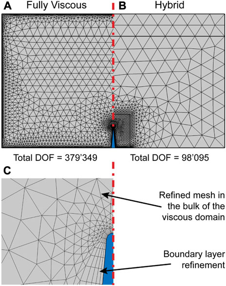
FIGURE 3. Comparison of the converged meshes of (A) the Fully Viscous model with the total DOF of 379′349 and (B) the Hybrid model with the total DOF of 98′095 at f = 720 kHz in water, with a = 1 mm, h = 100 μm, α = 10°, and b = 150 µm; (C) closeup of the mesh of the Hybrid model near the sharp-edge tip, where the viscous boundary layer mesh is distinguishable.

The convergence of representative models with respect to the mesh element size is discussed in Supplementary Material.

In the Fully Viscous model, the first-order pressure and velocity were discretized using cubic Lagrange and quartic Lagrange elements, respectively. The second-order pressure and velocity were discretized with quadratic and cubic elements, respectively. In the Hybrid model, cubic Lagrange elements were used for the first-order pressure in the LVM domain, while the pressure and velocity in the Fully Viscous domain were discretized with quadratic and cubic Lagrange elements, respectively. At the second order, the discretization was quadratic and cubic for pressure and velocity, respectively.

The results of numerical simulations are evaluated through the base variables (p₁, v₁, and $⟨{\mathit{v}}_2⟩$) as well as through the time- and space-averaged acoustic energy density [46]

$E_{\text{ac}}=\frac{1}{\mathrm{\Omega }}{\int }_{\mathrm{\Omega }}⟨\frac{1}{2{\rho }_0{c}_0^2}{p}_1^2+\frac{{\rho }_0}{2}\left({\mathit{v}}_1\cdot {\mathit{v}}_1\right)⟩\mathrm{d}\mathrm{\Omega },(35)$

within a spatial domain Ω that corresponds to the volume in a 3D or the area in a 2D configuration. The first term within $⟨\square ⟩$ in Eq. 35 represents the potential energy density, while the second term represents the kinetic energy density. In the LVM subdomains of Ω, v₁ is computed from Eq. 15.

3 Results

We study several cases using the described numerical models, which validate the Hybrid model on various 2D geometries in combination with fluidic channel resonances. In the last part, the benefit of the Hybrid model is demonstrated on the analysis of an exemplary 3D case that would have been very difficult if not impossible to model using preexisting approaches.

3.1 Rectangular channel in 2D

We first analyze a simple case of a 2D rectangular fluidic channel that is geometrically equivalent to the case presented in Figure 2, but without the sharp edge. The analysis, presented in Figure 4, compares the FLVM model and the Hybrid model against the Fully Viscous model, in order to validate the implementation in COMSOL Multiphysics and to estimate the baseline error caused by the coupling of Fully Viscous and LVM domains within the Hybrid model. In the Hybrid model, the Fully Viscous domain is defined with length b, while the LVM formulation is applied to the rest of the rectangular domain defined with length a, as specified in Figure 2.

FIGURE 4

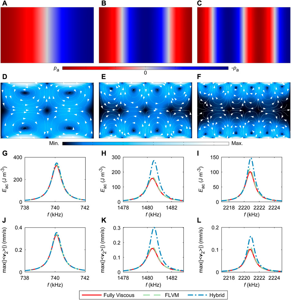
FIGURE 4. Different modeling approaches validated with a rectangular channel without the presence of a sharp edge. We compare the performance of the Fully Viscous model according to [15], the FLVM model from [22], and the Hybrid model outlined in Figure 2 that combines the two former approaches. The comparison is made for the first three resonance modes in water along the channel width a = 1 mm, with b = 200 μm; mode 1 is shown in (A), (D), (G), and (J); mode 2 in (B), (E), (H), and (K); and mode 3 in (C), (F), (I), and (L). The first row shows representative acoustic pressure fields (FLVM), the second row shows representative Eulerian streaming velocity fields (FLVM) with streamlines and arrows revealing the direction of the velocity, the third row shows the average acoustic energy density E_ac, and the fourth row shows the maximal magnitude of the Eulerian streaming velocity |⟨v₂⟩|. To support the build-up of the corresponding resonances, the excitation at x =±a/2 with v_a = 1 mm s⁻¹ is imposed in the same direction (in phase) for modes 1 and 3 and in the opposing directions (π phase shift) for mode 2.

The 2D geometry of the rectangular fluidic channel in Figure 4 is frequently used for studies in acoustofluidics [15, 25, 39, 46, 47]. The geometry is defined through the lengths a = 1 mm and b = 200 µm. Predictions of the three models are compared around the first three resonance modes across the width of the rectangular channel in the x-direction. We apply the excitation at x = ±a/2 with v_a = 1 mm s⁻¹ imposed in the same direction at both sides of the channel (in phase) to support the build-up of the resonance modes 1 (Figure 4A) and 3 (Figure 4C) across the channel width. For the resonance mode 2 in Figure 4B, the velocity v_a = 1 mm s⁻¹ is imposed in the opposing directions (π phase shift) at the two sides of the channel.

Qualitatively, the first- and second-order fields look the same for all models and modes; therefore, only reference normalized fields are shown in Figures 4A-F. The frequency sweeps around the three resonance frequencies in Figures 4G-L, which further validate our COMSOL Multiphysics implementation of the LVM, as particularly the FLVM model matches the Fully Viscous model perfectly. While the Hybrid model matches the Fully Viscous model well for all three modes in terms of the corresponding resonance frequency, it overestimates the acoustic energy density E_ac and maximal streaming velocity $\mathrm{m}\mathrm{a}\mathrm{x}\left(|⟨{\mathit{v}}_2⟩|\right)$. The error for the first mode is 7% and 6% for E_ac and $\mathrm{m}\mathrm{a}\mathrm{x}\left(|⟨{\mathit{v}}_2⟩|\right)$, respectively. In the case of the two higher modes, the errors reach up to 76%. The error comes from the coupling of the LVM with Fully Viscous domains and can be minimized by reducing the length of the boundary section that assumes a Fully viscous formulation and by positioning the Fully Viscous domain close to the pressure node (see Supplementary Material for further analysis). However, for frequencies away from the center of the resonance peak, the errors are minimized and all three models agree well.

3.2 Rectangular channel with a sharp-edge structure in 2D

In Figure 5, we look at the same 2D rectangular fluidic channel as in Figure 4, whereas a sharp edge has been added. A comparable geometry is featured in several prior experimental [2, 4, 7, 14] and numerical [2, 5, 25, 26] studies of sharp-edge acoustofluidics.

FIGURE 5

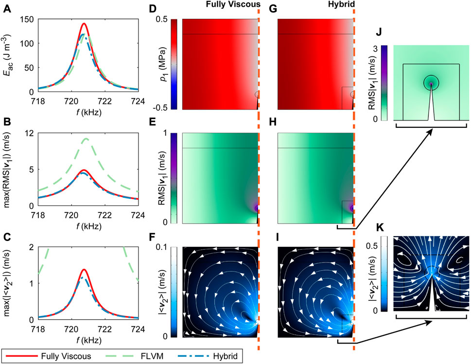
FIGURE 5. Different modeling approaches validated with a rectangular channel containing a sharp-edge structure. We compare the performance of the Fully Viscous model according to Muller et al. [15], the FLVM model from [22], and the Hybrid model outlined in Figure 2 that combines the two former approaches. The comparison is made for the first resonance mode in water along the channel width a = 1 mm, with h = 100 μm, b = 150 μm, and α = 10°. (A) Average acoustic energy density E_ac, (B) maximal root-mean-square acoustic velocity RMS|v₁|, and (C) maximal Eulerian streaming velocity magnitude |⟨v₂⟩|. (D), (G) Half of the acoustic pressure fields that are otherwise antisymmetric. (E), (H) Half of the root-mean-square acoustic velocity magnitudes that are otherwise symmetric. (F), (I) Half of the Eulerian streaming velocity fields that are otherwise symmetric. (J), (K) Zoomed-in fields corresponding to (H) and (I), respectively. (D)–(F) From the Fully Viscous model; (G)–(K) from the Hybrid model. All the displayed fields correspond to f = 720 kHz. The fields from the FLVM model are omitted, since they are erroneous due to the inherent assumptions of the model (as a note, the direction of the streaming velocity from the FLVM model is inverted relative to the actual pattern). The excitation is imposed in the same direction (in phase) at x =±a/2 with v_a = 1 mm s⁻¹.

We apply the excitation at x = ±a/2 with v_a = 1 mm s⁻¹ imposed in the same direction at both sides of the channel (in phase) to facilitate the build-up of the first resonance mode across the channel width. The first resonance mode was chosen for the analysis as it induces a pressure node and, thus, a velocity antinode at the location of the sharp-edge tip, producing strong sharp-edge phenomena.

The presence of the sharp edge shifts the resonance frequency of the first mode in Figure 5 from ∼ 740.1 kHz down to ∼ 720.8 kHz, when compared to a channel without the sharp edge in Figure 4. The lower resonance frequency in the rectangular fluidic channel featuring a sharp edge, compared to the channel without the sharp edge, was already observed in simulations in [26]. This frequency shift might be due to the increased path of waves, as they have to circumvent the sharp edge, analogously to the presence of other objects dispersed in an acoustic field that decrease the resonance frequency, for instance, bubbles [30].

Figure 5 reveals a good agreement between the Hybrid model and the Fully Viscous model, whereas the FLVM model quantitatively and qualitatively disagrees with the Fully Viscous model. The latter is expected based on the underlying assumptions of the LVM, and the FLVM model is, therefore, omitted from further analysis. At the resonance peak, the Hybrid model slightly underestimates the magnitude of the first-order fields, reflected in ∼16% lower E_ac maximum compared to the Fully Viscous model. Similarly, the maximal magnitude of the Eulerian streaming velocity is underestimated by ∼16% at the resonance peak. However, the agreement between the Hybrid model and the Fully Viscous model is very good away from the center of the resonance peak. Specifically, the difference in E_ac and $\mathrm{m}\mathrm{a}\mathrm{x}\left(|⟨{\mathit{v}}_2⟩|\right)$ is $<$ 5% for frequencies $>|\pm$ 2 kHz | from the center frequency of the peak.

In order to understand how the newly developed Hybrid model is compared to the Fully Viscous model in terms of the computational demand relative to an increasing size of the domain, we keep track of the DOF as the channel width a is increased. The results shown in Figure 6 present E_ac, $\mathrm{m}\mathrm{a}\mathrm{x}\left(|⟨{\mathit{v}}_2⟩|\right)$, and the DOF for the rectangular channel with a sharp edge from Figure 2 at f = 10 kHz and across the channel width range of 0.3 mm ≤ a ≤ 50 mm, making this a subwavelength problem (λ ≈ 150 mm). The results indicate a good agreement between the two models in terms of E_ac and $\mathrm{m}\mathrm{a}\mathrm{x}\left(|⟨{\mathit{v}}_2⟩|\right)$ across the whole range of a. Interestingly, the behavior below a ≈ 1 mm depends on a, while it remains independent of a for larger domain sizes. The DOF in the Fully Viscous model, however, significantly exceeds the DOF in the Hybrid model, with the DOF reaching $>40$-fold reduction as the domain size is increased, indicating the benefit of the Hybrid model.

FIGURE 6

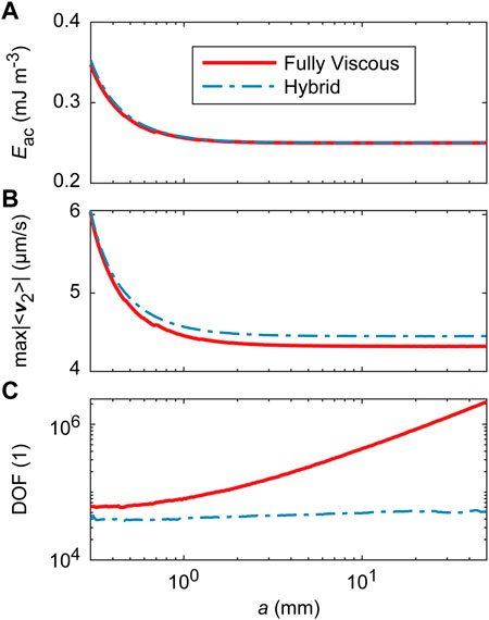
FIGURE 6. Influence of the channel width a on the performance of the Fully Viscous model and the Hybrid model for a subwavelength system with a sharp edge. The channel width is varied in the range of 0.3 mm ≤ a ≤ 50 mm at a fixed low frequency of f = 10 kHz to avoid channel resonances. The channel contains a single sharp edge, as indicated in Figure 2, with h = 100 μm, b = 150 μm, α = 10°, and the sharp-edge rounding radius of 0.3 µm. (A) Average acoustic energy density E_ac, (B) maximal Eulerian streaming velocity magnitude |⟨v₂⟩|, and (C) scaling of the DOF with the channel width. The excitation is imposed in the same direction (in phase) at x =±a/2, with a channel-width-dependent amplitude $v_{\mathrm{a}}=v_{\text{mid}}\cos \left[2xf\pi /c_0\right]$ that enforces a constant acoustic velocity amplitude v_mid = 1 mm s⁻¹ in the middle of the channel at the sharp edge.

To compare the scaling of the Hybrid model and the Fully Viscous model at higher frequencies, we vary a from 0.3 mm to 3.5 mm at f = 720 kHz. The results in Figure 7 reveal three resonances in the channel across the investigated range of a, with the first peak at a ≈ 1 mm corresponding to the resonance peak previously analyzed in Figure 5. The two models match very well in terms of E_ac and $\mathrm{m}\mathrm{a}\mathrm{x}\left(|⟨{\mathit{v}}_2⟩|\right)$. The DOF generally exceed those from Figure 6 due to the higher frequency, and the DOF in the Hybrid model again show a significant up to $\sim 11$-fold decrease relative to the DOF in the Fully Viscous model.

FIGURE 7

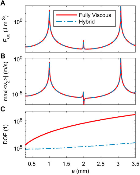
FIGURE 7. Influence of the channel width a on the performance of the Fully Viscous model and the Hybrid model for a resonant system with a sharp edge. Channel width is varied in the range of 0.3 mm ≤ a ≤ 3.5 mm at a fixed frequency of f = 720 kHz to induce channel resonances. The channel contains a single sharp edge, as indicated in Figure 2, with h = 100 μm, b = 150 μm, α = 10°, and the sharp-edge rounding radius of δ/2. (A) Average acoustic energy density E_ac, (B) maximal Eulerian streaming velocity magnitude |⟨v₂⟩|, and (C) scaling of the DOF with the channel width. The excitation is imposed in the same direction (in phase) at x =±a/2, with a fixed amplitude v_a = 1 mm s⁻¹. The imposed excitation supports the odd resonances (modes 1, 3, … ) that have a symmetric acoustic velocity field about the plane of the symmetry x =0 at the sharp edge.

3.3 Sharp-edge-based micropump in 2D

The main advantage of the developed Hybrid model is the ability to model larger systems that feature sharp-edge structures. We analyze the performance of the Hybrid model for a larger system in Figure 8, in the case of a 2D acoustofluidic micropump inspired by [9] that is capable of fluid pumping and mixing due to the sharp-edge streaming, as well as microparticle/cell focusing and trapping by the acoustic radiation force due to the fluidic channel resonances.

FIGURE 8

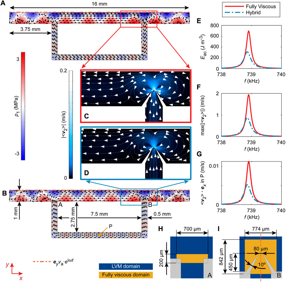
FIGURE 8. Different modeling approaches validated on a complex 2D geometry containing a pair of sharp edges that can facilitate pumping. The geometry is inspired by the experimental device from [9]. We compare the performance of the Fully Viscous model and the Hybrid model that combines the Fully Viscous domain with the limiting velocity method domain. The comparison is made for one of the resonance modes in water with the dimensions of the rigid channels defined in (A), (B), (H), and (I), where (H) and (I) show the Fully Viscous domains. The acoustic pressure and the streamlines of the Eulerian streaming velocity are shown in (A) for the Fully Viscous model and in (B) for the Hybrid model and (C) and (D) show the respective zoomed-in Eulerian streaming fields near the pair of sharp edges. The compared fields correspond to f = 738.85 kHz, where (E) shows the average acoustic energy density E_ac, (F) shows the maximal Eulerian streaming velocity magnitude |⟨v₂⟩|, and (G) shows the x-component of the Eulerian streaming velocity in point P, defined in (B). The excitation in a form of an oscillatory velocity in the y-direction with an amplitude v_a = 1 mm s⁻¹ is imposed on the whole uppermost boundary.

Similar to the previous results, the behavior predicted by the Fully Viscous model and the Hybrid model matches qualitatively and quantitatively, except for the resonance peak, where the Hybrid model underestimates the magnitude of acoustic fields.

3.4 Rectangular channel with a sharp-edge structure in 3D

Finally, we demonstrate the capability of our efficient modeling approach by solving a high-frequency acoustic streaming problem in 3D using a Hybrid model with the geometry from Figure 2 extruded to a depth of d. The exemplary mesh and results are shown in Figure 9.

FIGURE 9

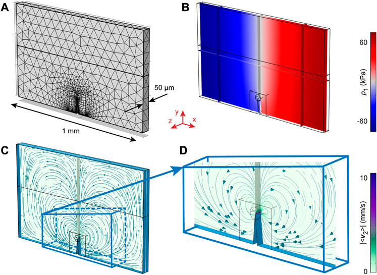
FIGURE 9. The Hybrid model of a rectangular channel containing a sharp-edge structure in 3D. An analysis is performed near the first resonance mode in water along the channel width a = 1 mm, with h = 100 μm, b = 150 μm, d = 50 μm, and α = 10°. (A) The mesh, (B) the first-order pressure p₁, (C) the Eulerian streaming velocity pattern, and (D) the zoomed-in streaming field corresponding to (C). The analysis of the pressure and streaming velocity fields in (B)–(D) is performed at the middle xy-plane (at z = d/2), with some additional xz- and yz-planes for orientation. All the displayed fields correspond to f = 720 kHz. The excitation is imposed in the same direction (in phase) at x =±a/2 with v_a = 1 mm s⁻¹.

We apply the 3D model to study the influence of the depth d on the Eulerian streaming pattern on the xy-plane at z = d/2 in Figure 10. The results show that the pattern is visibly affected by the presence of the front (z = d) and back (z = 0) covers when d = 10 µm in Figure 10A, but the pattern gradually converges to the streaming pattern in the 2D model from Figure 5 as d is increased to 100 µm in Figure 10D. However, as shown in Figure 10E, the maximal Eulerian streaming velocity magnitude remains impaired by the 3D effects even at d = 100 μm, when compared to the magnitudes from a comparable 2D configuration at f = 720 kHz from Figure 5C.

FIGURE 10

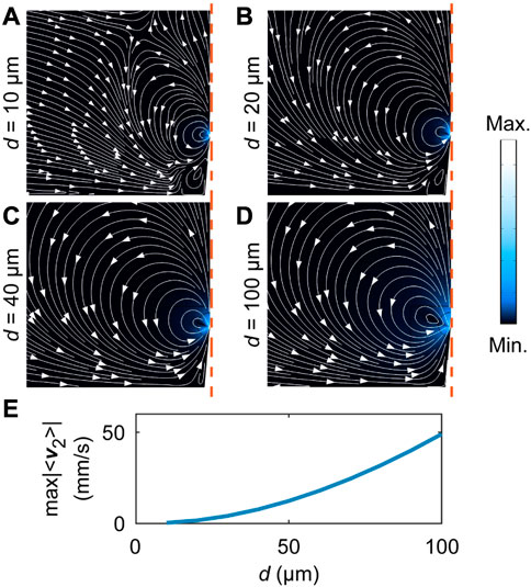
FIGURE 10. Influence of the channel depth d on the sharp-edge streaming pattern at the middle xy-plane (at z = d/2), studied with the Hybrid 3D model. The channel depth is varied from d = 10 µm in (A) to d = 100 µm in (D) at a fixed frequency of f = 720 kHz. The corresponding maximal Eulerian streaming velocity |⟨v₂⟩| is shown in (E). The channel contains a single sharp edge, as indicated in Figure 2, with h = 100 μm, b = 150 μm, α = 10°, and the sharp-edge rounding radius of δ/2. (A)–(D) Eulerian streaming velocity magnitude |⟨v₂⟩|. The excitation is imposed in the same direction (in phase) at x =±a/2, with an amplitude of v_a = 1 mm s⁻¹.

4 Discussion

We have demonstrated that the novel Hybrid model, combining the Fully Viscous modeling of the acoustic phenomena [15] near sharp edges with the efficient modeling of the viscous boundary layers according to [22] in the rest of the device, provides up to $>40$-fold reduction in the required DOF in 2D validation studies while capturing the relevant physics. Furthermore, this approach enables the modeling of 3D sharp-edge phenomena at high frequencies, where the viscous boundary layer thickness δ reduces to the rounding radius of sharp edges or below.

While the novel Hybrid model introduces a quantitative error on the estimated magnitude of fields at the resonance peaks, it correctly predicts the qualitative behavior throughout the modeled device. This is of no concern for problems that do not involve resonances in the fluidic channels, e.g., the configurations from [2, 5, 14]. Sharp-edge-based devices operating at higher frequencies, such as the multifunctional chip reported by [9], can still be effectively modeled, as demonstrated in Figure 8. Shortcomings in terms of erroneous magnitudes at resonances are not too important, since the underlying total damping defining the quality of a given resonance is generally difficult to model anyway and can vary due to a plethora of experimental conditions [19], such as the temperature, material damping, damping in the connecting glue layers, and many more.

The relative error of the Hybrid model is for a given resonance similar for both analyzed quantities, E_ac and $\mathrm{m}\mathrm{a}\mathrm{x}\left(|⟨{\mathit{v}}_2⟩|\right)$. This implies that the error originates from the computation of the first-order fields, since both quantities rely on the square of a first-order quantity—E_ac directly, while $\mathrm{m}\mathrm{a}\mathrm{x}\left(|⟨{\mathit{v}}_2⟩|\right)$ depends the square of the first-order velocity as a source term in Eq. 7 and as a boundary condition through Eq. 9.

Our Hybrid model allows the study of 3D sharp-edge effects, as demonstrated in Figure 10, where we showed that the 3D effects in the quasi-2D geometry are limited to a certain depth, as previously hypothesized in [5]. This provides the justification for the use of 2D models when modeling quasi-2D channels of lab-on-a-chip devices that typically exceed the depth of 100 µm.

The herein introduced Hybrid modeling approach can be used to aid the emerging field of sharp-edge acoustofluidics. In the latter, sharp-edge structures such as needles or wedges in microfluidic devices are excited with ultrasound for a wide range of applications, ranging from propulsion of microrobots [48–50] and enhanced drug delivery [27] to advanced lab-on-a-chip technology involving sharp-edge-based micropumps and micromixers [3, 8, 9, 12–14, 51].

Data availability statement

The original contributions presented in the study are included in the article/Supplementary Material; further inquiries can be directed to the corresponding author.

Author contributions

AP and LR implemented the numerical models and carried out the numerical studies. AP and CH supervised LR. AP provided the initial draft of the manuscript. JD supervised the project. All authors contributed substantially to scientific discussion and to the writing of the manuscript.

Funding

The authors gratefully acknowledge the financial support of the Swiss Federal Institute of Technology Zurich (ETH Zurich) and open-access funding by ETH Zurich.

Acknowledgments

The authors would like to thank COMSOL AB and Jonas H. Jørgensen for their support. They would also like to thank Luca Rosenthaler for his work on the implementation of the limiting velocity method in COMSOL Multiphysics.

Conflict of interest

The authors declare that the research was conducted in the absence of any commercial or financial relationships that could be construed as a potential conflict of interest.

Publisher’s note

All claims expressed in this article are solely those of the authors and do not necessarily represent those of their affiliated organizations, or those of the publisher, the editors, and the reviewers. Any product that may be evaluated in this article, or claim that may be made by its manufacturer, is not guaranteed or endorsed by the publisher.

Supplementary material

The Supplementary Material for this article can be found online at: https://www.frontiersin.org/articles/10.3389/fphy.2023.1182532/full#supplementary-material

References

1. Bruus H, Dual J, Hawkes J, Hill M, Laurell T, Nilsson J, et al. Forthcoming lab on a chip tutorial series on acoustofluidics: Acoustofluidics—Exploiting ultrasonic standing wave forces and acoustic streaming in microfluidic systems for cell and particle manipulation. Lab Chip (2011) 11:3579–80. doi:10.1039/c1lc90058g

PubMed Abstract | CrossRef Full Text | Google Scholar

2. Ovchinnikov M, Zhou J, Yalamanchili S. Acoustic streaming of a sharp edge. The J Acoust Soc America (2014) 136:22–9. doi:10.1121/1.4881919

PubMed Abstract | CrossRef Full Text | Google Scholar

3. Nama N, Huang PH, Huang TJ, Costanzo F. Investigation of acoustic streaming patterns around oscillating sharp edges. Lab Chip (2014) 14:2824–36. doi:10.1039/c4lc00191e

PubMed Abstract | CrossRef Full Text | Google Scholar

4. Doinikov AA, Gerlt MS, Pavlic A, Dual J. Acoustic streaming produced by sharp-edge structures in microfluidic devices. Microfluidics and Nanofluidics (2020) 24:32. doi:10.1007/s10404-020-02335-5

CrossRef Full Text | Google Scholar

5. Zhang C, Guo X, Royon L, Brunet P. Unveiling of the mechanisms of acoustic streaming induced by sharp edges. Phys Rev E (2020) 102:043110. doi:10.1103/physreve.102.043110

PubMed Abstract | CrossRef Full Text | Google Scholar

6. Leibacher I, Hahn P, Dual J. Acoustophoretic cell and particle trapping on microfluidic sharp edges. Microfluidics and Nanofluidics (2015) 19:923–33. doi:10.1007/s10404-015-1621-1

CrossRef Full Text | Google Scholar

7. Doinikov AA, Gerlt MS, Dual J. Acoustic radiation forces produced by sharp-edge structures in microfluidic systems. Phys Rev Lett (2020) 124:154501. doi:10.1103/physrevlett.124.154501

PubMed Abstract | CrossRef Full Text | Google Scholar

8. Huang PH, Nama N, Mao Z, Li P, Rufo J, Chen Y, et al. A reliable and programmable acoustofluidic pump powered by oscillating sharp-edge structures. Lab Chip (2014) 14:4319–23. doi:10.1039/c4lc00806e

PubMed Abstract | CrossRef Full Text | Google Scholar

9. Pavlic A, Harshbarger CL, Rosenthaler L, Snedeker JG, Dual J. Sharp-edge-based acoustofluidic chip capable of programmable pumping, mixing, cell focusing and trapping. Phys Fluids (2023) 35:022006. doi:10.1063/5.0133992

CrossRef Full Text | Google Scholar

10. Nivedita N, Garg N, Lee AP, Papautsky I. A high throughput microfluidic platform for size-selective enrichment of cell populations in tissue and blood samples. Analyst (2017) 142:2558–69. doi:10.1039/c7an00290d

PubMed Abstract | CrossRef Full Text | Google Scholar

11. Garg N, Westerhof TM, Liu V, Liu R, Nelson EL, Lee AP. Whole-blood sorting, enrichment and in situ immunolabeling of cellular subsets using acoustic microstreaming. Microsystems and Nanoengineering (2018) 4:17085. doi:10.1038/micronano.2017.85

CrossRef Full Text | Google Scholar

12. Huang PH, Xie Y, Ahmed D, Rufo J, Nama N, Chen Y, et al. An acoustofluidic micromixer based on oscillating sidewall sharp-edges. Lab Chip (2013) 13:3847–52. doi:10.1039/c3lc50568e

PubMed Abstract | CrossRef Full Text | Google Scholar

13. Nama N, Huang PH, Huang TJ, Costanzo F. Investigation of micromixing by acoustically oscillated sharp-edges. Biomicrofluidics (2016) 10:024124. doi:10.1063/1.4946875

PubMed Abstract | CrossRef Full Text | Google Scholar

14. Zhang C, Guo X, Brunet P, Costalonga M, Royon L. Acoustic streaming near a sharp structure and its mixing performance characterization. Microfluidics and Nanofluidics (2019) 23:104. doi:10.1007/s10404-019-2271-5

CrossRef Full Text | Google Scholar

15. Muller PB, Barnkob R, Jensen MJH, Bruus H. A numerical study of microparticle acoustophoresis driven by acoustic radiation forces and streaming-induced drag forces. Lab Chip (2012) 12:4617–27. doi:10.1039/c2lc40612h

PubMed Abstract | CrossRef Full Text | Google Scholar

16. Rayleigh L. On the circulation of air observed in Kundt’s tubes, and on some allied acoustical problems. Phil Trans R Soc Lond (1884) 175:1–21. doi:10.1098/rstl.1884.0002

CrossRef Full Text | Google Scholar

17. Nyborg WL. Acoustic streaming due to attenuated plane waves. The J Acoust Soc America (1953) 25:68–75. doi:10.1121/1.1907010

CrossRef Full Text | Google Scholar

18. Nyborg WL. Acoustic streaming near a boundary. J Acoust Soc America (1958) 30:329–39. doi:10.1121/1.1909587

CrossRef Full Text | Google Scholar

19. Hahn P, Leibacher I, Baasch T, Dual J. Numerical simulation of acoustofluidic manipulation by radiation forces and acoustic streaming for complex particles. Lab Chip (2015) 15:4302–13. doi:10.1039/c5lc00866b

PubMed Abstract | CrossRef Full Text | Google Scholar

20. Lei J, Glynne-Jones P, Hill M. Acoustic streaming in the transducer plane in ultrasonic particle manipulation devices. Lab Chip (2013) 13:2133–43. doi:10.1039/c3lc00010a

PubMed Abstract | CrossRef Full Text | Google Scholar

21. Lei J, Hill M, Glynne-Jones P. Numerical simulation of 3d boundary-driven acoustic streaming in microfluidic devices. Lab Chip (2014) 14:532–41. doi:10.1039/c3lc50985k

PubMed Abstract | CrossRef Full Text | Google Scholar

22. Bach JS, Bruus H. Theory of pressure acoustics with viscous boundary layers and streaming in curved elastic cavities. J Acoust Soc America (2018) 144:766–84. doi:10.1121/1.5049579

PubMed Abstract | CrossRef Full Text | Google Scholar

23. Joergensen JH, Bruus H. Theory of pressure acoustics with thermoviscous boundary layers and streaming in elastic cavities. J Acoust Soc America (2021) 149:3599–610. doi:10.1121/10.0005005

CrossRef Full Text | Google Scholar

24. Skov NR, Bach JS, Winckelmann BG, Bruus H. 3d modeling of acoustofluidics in a liquid-filled cavity including streaming, viscous boundary layers, surrounding solids, and a piezoelectric transducer. Aims Math (2019) 4:99–111. doi:10.3934/math.2019.1.99

CrossRef Full Text | Google Scholar

25. Lei J, Hill M, de León Albarrán CP, Glynne-Jones P. Effects of micron scale surface profiles on acoustic streaming. Microfluidics and Nanofluidics (2018) 22:140–14. doi:10.1007/s10404-018-2161-2

CrossRef Full Text | Google Scholar

26. Zhou Y. Effect of microchannel protrusion on the bulk acoustic wave-induced acoustofluidics: Numerical investigation. Biomed Microdevices (2022) 24:7–12. doi:10.1007/s10544-021-00608-6

CrossRef Full Text | Google Scholar

27. Perra E, Hayward N, Pritzker KP, Nieminen HJ. An ultrasonically actuated needle promotes the transport of nanoparticles and fluids. J Acoust Soc America (2022) 152:251–65. doi:10.1121/10.0012190

CrossRef Full Text | Google Scholar

28. Pavlic A, Nagpure P, Ermanni L, Dual J. Influence of particle shape and material on the acoustic radiation force and microstreaming in a standing wave. Phys Rev E (2022) 106:015105. doi:10.1103/physreve.106.015105

PubMed Abstract | CrossRef Full Text | Google Scholar

29. Orosco J, Friend J. Modeling fast acoustic streaming: Steady-state and transient flow solutions. Phys Rev E (2022) 106:045101. doi:10.1103/physreve.106.045101

PubMed Abstract | CrossRef Full Text | Google Scholar

30. Hamilton MF, Blackstock DT. Nonlinear acoustics. San Diego: Academic press San Diego (1998).

Google Scholar

31. Lighthill J. Acoustic streaming. J Sound Vibration (1978) 61:391–418. doi:10.1016/0022-460x(78)90388-7

CrossRef Full Text | Google Scholar

32. Bruus H. Theoretical Microfluidics, 18. Oxford University Press (2007).

Google Scholar

33. Nyborg WLM. Acoustic streaming. In: Physical acoustics, 2. Elsevier (1965). p. 265–331.

CrossRef Full Text | Google Scholar

34. Doinikov AA, Thibault P, Marmottant P. Acoustic streaming in a microfluidic channel with a reflector: Case of a standing wave generated by two counterpropagating leaky surface waves. Phys Rev E (2017) 96:013101. doi:10.1103/physreve.96.013101

PubMed Abstract | CrossRef Full Text | Google Scholar

35. Doinikov AA, Thibault P, Marmottant P. Acoustic streaming induced by two orthogonal ultrasound standing waves in a microfluidic channel. Ultrasonics (2018) 87:7–19. doi:10.1016/j.ultras.2018.02.002

PubMed Abstract | CrossRef Full Text | Google Scholar

36. Baasch T, Doinikov AA, Dual J. Acoustic streaming outside and inside a fluid particle undergoing monopole and dipole oscillations. Phys Rev E (2020) 101:013108. doi:10.1103/physreve.101.013108

PubMed Abstract | CrossRef Full Text | Google Scholar

37. Andrews DG, McIntyre M. An exact theory of nonlinear waves on a Lagrangian-mean flow. J Fluid Mech (1978) 89:609–46. doi:10.1017/s0022112078002773

CrossRef Full Text | Google Scholar

38. Vanneste J, Bühler O. Streaming by leaky surface acoustic waves. Proc R Soc A: Math Phys Eng Sci (2011) 467:1779–800. doi:10.1098/rspa.2010.0457

CrossRef Full Text | Google Scholar

39. Hamilton MF, Ilinskii YA, Zabolotskaya EA. Acoustic streaming generated by standing waves in two-dimensional channels of arbitrary width. J Acoust Soc America (2003) 113:153–60. doi:10.1121/1.1528928

PubMed Abstract | CrossRef Full Text | Google Scholar

40. Pavlic A, Dual J. On the streaming in a microfluidic Kundt’s tube. J Fluid Mech (2021) 911:A28. doi:10.1017/jfm.2020.1046

CrossRef Full Text | Google Scholar

41. Comsol AB. COMSOL Multiphysics 5.6 (2020). Available at: www.comsol.com (March 08, 2023).

Google Scholar

42. Baasch T, Pavlic A, Dual J. Acoustic radiation force acting on a heavy particle in a standing wave can be dominated by the acoustic microstreaming. Phys Rev E (2019) 100:061102. doi:10.1103/physreve.100.061102

PubMed Abstract | CrossRef Full Text | Google Scholar

43. Riaud A, Baudoin M, Matar OB, Thomas JL, Brunet P. On the influence of viscosity and caustics on acoustic streaming in sessile droplets: An experimental and a numerical study with a cost-effective method. J Fluid Mech (2017) 821:384–420. doi:10.1017/jfm.2017.178

CrossRef Full Text | Google Scholar

44. Bach JS, Bruus H. Bulk-driven acoustic streaming at resonance in closed microcavities. Phys Rev E (2019) 100:023104. doi:10.1103/physreve.100.023104

PubMed Abstract | CrossRef Full Text | Google Scholar

45. Holmes M, Parker N, Povey M. Temperature dependence of bulk viscosity in water using acoustic spectroscopy. J Phys Conf Ser (2011) 269:012011. doi:10.1088/1742-6596/269/1/012011

CrossRef Full Text | Google Scholar

46. Muller PB, Bruus H. Theoretical study of time-dependent, ultrasound-induced acoustic streaming in microchannels. Phys Rev E (2015) 92:063018. doi:10.1103/physreve.92.063018

PubMed Abstract | CrossRef Full Text | Google Scholar

47. Bruus H. Acoustofluidics 2: Perturbation theory and ultrasound resonance modes. Lab Chip (2012) 12:20–8. doi:10.1039/c1lc20770a

PubMed Abstract | CrossRef Full Text | Google Scholar

48. Kaynak M, Ozcelik A, Nama N, Nourhani A, Lammert PE, Crespi VH, et al. Acoustofluidic actuation of in situ fabricated microrotors. Lab Chip (2016) 16:3532–7. doi:10.1039/c6lc00443a

PubMed Abstract | CrossRef Full Text | Google Scholar

49. Kaynak M, Ozcelik A, Nourhani A, Lammert PE, Crespi VH, Huang TJ. Acoustic actuation of bioinspired microswimmers. Lab Chip (2017) 17:395–400. doi:10.1039/c6lc01272h

PubMed Abstract | CrossRef Full Text | Google Scholar

50. Dillinger C, Nama N, Ahmed D. Ultrasound-activated ciliary bands for microrobotic systems inspired by starfish. Nat Commun (2021) 12:6455. doi:10.1038/s41467-021-26607-y

PubMed Abstract | CrossRef Full Text | Google Scholar

51. Chen Z, Liu P, Zhao X, Huang L, Xiao Y, Zhang Y, et al. Sharp-edge acoustic microfluidics: Principles, structures, and applications. Appl Mater Today (2021) 25:101239. doi:10.1016/j.apmt.2021.101239

CrossRef Full Text | Google Scholar