Fractional solitons: New phenomena and exact solutions

The fractional solitons have demonstrated many new phenomena, which cannot be explained by the traditional solitary wave theory. This paper studies some famous fractional wave equations including the fractional KdV–Burgers equation and the fractional approximate long water wave equation by a modified tanh-function method. The solving process is given in details, and new solitons can be rigorously explained by the obtained exact solutions. This paper offers a new window for studying fractional solitons.

1 Introduction

A fractional solitary wave [1] has some special properties which cannot be explained by the traditional soliton theory. The traditional soliton is a single wave with the same shape in propagation, while the fractional soliton has some amazing memory and non-local properties, which means the present wave morphology depends upon its history. This is caused by the intrinsic property of the fractional derivative [2]. The fractal solitary waves, on the other hand, are waves traveling along an unsmooth boundary [3, 4]. And the fractal solitary wave has the local property, the unsmooth boundary affects its wave shape. Here, the two-scale fractal theory [5, 6] is adopted to figure out the basic property of the unsmooth boundary.

This paper focuses on fractional solitons, which can describe physical phenomena more accurately and reflect their intrinsic properties deeply. Therefore, fractional solitons have attracted increasing attention from both physics and oceanography. For example, shallow water waves [7, 8] can describe the effects of waves in the ocean better than other mathematical models. Shallow water waves are fluctuations in the ocean with wavelengths much greater than the depth of the water (usually more than 25 times), and the dispersion of water waves is one of the key properties in many shallow water wave models, which has obvious memory property. Fractional shallow water equations can describe the propagation of waves in dispersed media and model the hydrodynamics of lakes, estuaries, tidal stalls, and coastal waves, as well as deep-ocean tides. These fractional differential equations have a significant impact on the study of fluid motion in ocean waves and the soliton theory as well; however, a serious bottleneck was hit, that is, the fractional model is extremely difficult to be solved analytically. Therefore, many scholars focused on using different methods to find fractional solitons. For instance, the first integral method [9], the fractional sub-equation method [10], the homotopy perturbation method [11-13] and its modifications, Mohand transform–homotopy perturbation method [14, 15], two-scale transform–-homotopy perturbation method [16], Laplace transform–homotopy perturbation method [17], Li–He’s modified homotopy perturbation method [18-20], the tanh-function method [21, 22] and its modification—tanh function expansion method [23]—and modified extended tanh-function method [24,25]. It is worth mentioning that fractional complex transform was first proposed by [26]; it can convert fractional differential equations directly into ordinary differential equations. This method makes a significant contribution to finding exact solutions of fractional differential equations, and it was applied to gain insights into physical properties of the time-fractional Schrodinger equation [27] and the time-fractional Camassa–Holm equation [28].

In the current article, our concern is to find some exact solutions of the following two non-linear FPDEs via the modified extended tanh-function method with the fractional complex transform.

1) The time-fractional KdV–Burgers (KdVB) equation of the form [29

$\frac{{\partial }^{\eta }u}{\partial t^{\eta }}+wu\frac{\partial u}{\partial x}+\rho \frac{{\partial }^{2}u}{\partial x^2}+s\frac{{\partial }^{3}u}{\partial x^3}=0,(1)$

where w, ρ, and s are real constants and 0$<\eta <$1. The KdVB equation (η = 1) is a well-known mathematical model for describing waves on shallow water surfaces; it plays an essential role in both applied mathematics and physics. This equation can be used to describe and analyze a few foremost physical contents related to liquids, dispersion, viscosity, and wave dynamics. For example, it is used to study the spread of waves in elastic tubes filled with viscous fluids [30] and to analyze the propagation of wave-like pores in shallow water [31].

However, with the increasing irregularities and non-linearities in wave motion observed by other scholars, the broader outlook establishment for this model is necessary. Therefore, an increasing number of scholars began to study the extended classical model into a new model with time-fractional derivatives to deal with what the traditional KdVB equation (η = 1) cannot do.

There have been some common methods to solve fractional KdVB equations. For instance, [32] extended the homotopy perturbation method to solve time-space fractional equations. [29] applied the residual power series method (RPSM) for finding approximate solutions of the time-fractional KdVB equation. [33] solved the time-fractional KdVB equation numerically by the Petrov–Galerkin method.

2) The fractional approximate long water wave equation is given as [34]

$\begin{array}{cc}\hfill & D_t^{\eta }u-u{D}_x^{\eta }u-D_x^{\eta }v+a{D}_x^{2\eta }u=0,\hfill \\ \hfill & D_t^{\eta }v-D_x^{\eta }\left(uv\right)-a{D}_x^{2\eta }v=0,\hfill \end{array}(2)$

where 0$<\eta <$1 and a is a real parameter. As a famous equation to describe the propagation of shallow water waves, it is also important for its amazing fractional solitons, so its exact solutions are much needed to gain insights deeply into the properties of the fractional solitary waves. Up to now, some explicit solutions appeared in the literature, for instance, [34] found three traveling wave solutions by the fractional sub-equation method, [35] obtained an exact solution by using the (G’/G)-method, and [36] also constructed an exact solution by the generalized Kudryashov method. Although much achievement was obtained, its full breathtaking panorama has not been offered yet.

The article is divided into the following sections: First, an introduction is given to the basic knowledge in Section 2; second, in Section 3, the general steps for the solution are given in detail; and finally, the applications and the conclusions are organized in Section 4 and Section 5, respectively.

2 Preliminaries

Regarding the definition of fractional derivatives, many mathematicians started from different perspectives and gave different definitions. Here are some definitions.

1) Caputo fractional derivative [37, 38]:

$D_x^{\eta }\left[f\left(x\right)\right]=\frac{1}{\mathrm{\Gamma }\left(n-\eta \right)}{\int }_0^x{\left(x-t\right)}^{n-\eta -1}\frac{{\text{d}}^{n}f\left(t\right)}{\text{d}{t}^n}\text{d}t.(3)$

2) Jumarie’s modified Riemann–Liouville (R–L) fractional derivative [39]:

$D_t^{\eta }g\left(t\right)=\left\{\begin{array}{cc}\frac{1}{\mathrm{\Gamma }\left(1-\eta \right)}{\int }_0^t{\left(t-\xi \right)}^{-\eta -1}\left(g\left(\xi \right)-g\left(0\right)\right)\mathrm{d}\xi ,\hfill & \eta <0,\hfill \\ \frac{1}{\mathrm{\Gamma }\left(1-\eta \right)}\frac{\mathrm{d}}{\mathrm{d}t}{\int }_0^t{\left(t-\xi \right)}^{-\eta }\left(g\left(\xi \right)-g\left(0\right)\right)\mathrm{d}\xi ,\hfill & 0<\eta <1,\hfill \\ {\left(g^{\left(n\right)}\left(t\right)\right)}^{\left(\eta -n\right)},\hfill & n\le \eta <n+1,n\ge 1,\hfill \end{array}\right.(4)$

where

$\mathrm{\Gamma }\left(\eta \right)={\int }_0^{+\infty }{x}^{\eta -1}{e}^{-x}dx,\eta >0.(5)$

(3) He’s fractional derivative [20, 40]:

$D_t^{\eta }f=\frac{1}{\mathrm{\Gamma }\left(n-\eta \right)}\frac{d^n}{d{t}^n}{\int }_{t_o}^t{\left(s-t\right)}^{n-\eta -1}\left[f_0\left(s\right)-f\left(s\right)\right]ds,(6)$

where f₀(x) is a known function.

4) Two-scale fractal derivative [41, 42]:

$\frac{\partial w}{\partial t^{\eta }}\left(t^{\eta }\right)=\mathrm{\Gamma }\left(1+\eta \right)\underset{t-t_0=4t,△\ne 0}{\lim }\frac{w\left(t^{\eta }\right)-w\left(t_0^{\eta }\right)}{{\left(t-t_0\right)}^{\eta }},(7)$

where △t is the period required for the motion through a gap of a porous space.

In addition, there are other famous derivatives in the literature such as the Atangana–Baleanu derivative with non-local and non-singular kernel [43, 44]. In this paper, we adopt the Jumarie’s modified R–L derivative definition. Some of its important properties are as follows:

$D_t^{\eta }{t}^m=\frac{\mathrm{\Gamma }\left(1+m\right)}{\mathrm{\Gamma }\left(1+m-\eta \right)}{t}^{m-\eta },(8)$

$D_t^{\eta }\left(cg\left(x\right)\right)=c{D}_t^{\eta }g\left(x\right),cisaconstant,(9)$

$D_t^{\eta }\left\{g\left(\omega \right)+f\left(\omega \right)\right\}=D_t^{\eta }g\left(\omega \right)+D_t^{\eta }f\left(w\right).(10)$

3 Basic idea of the modified tanh-function expansion method

Considering the following equation

$P\left(u,D_t^{\eta }u,D_x^{\gamma }u,D_t^{\eta }{D}_t^{\eta }u,D_t^{\eta }{D}_x^{\gamma }u,D_x^{\gamma }{D}_x^{\gamma }u,\cdots \right)=0,\left(0<\eta ,\gamma <1\right),(11)$

where $D_t^{\eta }u,D_x^{\gamma }u,D_t^{\eta }{D}_t^{\eta }u,D_t^{\eta }{D}_x^{\gamma }u\cdots$ are the modified R–L fractional derivatives. P presents the polynomial function. To solve this equation, by using the modified tanh-function expansion method, we divide the solution processes into three steps.

Step 1: Using the fractional complex transformation [26, 45]

$\begin{array}{cc}\hfill & u\left(x,t\right)=u\left(\zeta \right),\hfill \\ \hfill & \zeta =\frac{l{x}^{\gamma }}{\mathrm{\Gamma }\left(\gamma +1\right)}+\frac{k{t}^{\eta }}{\mathrm{\Gamma }\left(\eta +1\right)},\hfill \end{array}(12)$

where l and k are constants and l, k ≠ 0. By the chain rule [45],

$\begin{array}{cc}\hfill & D_t^{\eta }u={\sigma }_t\frac{\partial u\left(\zeta \right)}{\mathrm{d}\zeta }{D}_t^{\eta }\zeta ,D_x^{\eta }u={\sigma }_x\frac{\partial u\left(\zeta \right)}{\mathrm{d}\zeta }{D}_x^{\eta }\zeta ,\hfill \\ \hfill & D_t^{2\eta }u={\left({\sigma }_t\right)}^2\frac{{\partial }^{2}u\left(\zeta \right)}{\mathrm{d}{\zeta }^2}{D}_t^{2\eta }\zeta ,D_x^{2\eta }u={\left({\sigma }_x\right)}^2\frac{{\partial }^{2}u\left(\zeta \right)}{\mathrm{d}{\zeta }^2}{D}_x^{2\eta }\zeta ,\hfill \end{array}(13)$

where σ_t and σ_x are sigma indices. We take σ_t = σ_x = L, where L is a constant. Then, substituting Eqs 12 and 13 into Eq. 11, we obtain a non-linear ODE that contains only variable ζ:

$D\left(u,u^{\prime },u^{″}\cdots \right)=0,(14)$

where $u^{\prime }=\frac{\mathrm{d}u}{\mathrm{d}\zeta },u^{″}=\frac{{\mathrm{d}}^{2}u}{\mathrm{d}{\zeta }^2}\cdots$ and D presents the polynomial function.

Step 2: Supposing Eq. 14 has the solution as Eq. 15

$u\left(\zeta \right)=\sum _{i=0}^n{a}_i{\mathrm{\Phi }}^i\left(\zeta \right),(15)$

where Φ is a function about ζ, and it satisfies the Riccati equation

${\mathrm{\Phi }}^{\prime }=\tau +{\mathrm{\Phi }}^2,(16)$

τ is a constant, and a_i(i = 0, 1, 2, … , n) are undetermined constant. n is a balancing parameter which is determined by the homogeneous balance method. Φ has the following three types of solutions according to the different values of constant τ

$\left\{\begin{array}{cc}\mathrm{\Phi }=-\sqrt{-\tau }\tanh \sqrt{-\tau }\zeta ,\hfill & \tau <0,\hfill \\ \mathrm{\Phi }=-\sqrt{-\tau }\coth \sqrt{-\tau }\zeta ,\hfill & \tau <0,\hfill \\ \mathrm{\Phi }=\sqrt{\tau }\tan \sqrt{\tau }\zeta ,\hfill & \tau >0,\hfill \\ \mathrm{\Phi }=\sqrt{\tau }\cot \sqrt{\tau }\zeta ,\hfill & \tau >0,\hfill \\ \mathrm{\Phi }=-\frac{1}{\zeta },\hfill & \tau =0.\hfill \end{array}\right.(17)$

Step 3: Substituting Eq. 15 and 16 into Eq. 14, we obtain an iteration formulation to obtain the polynomial of Φ. Then, we get the algebraic equations about a_i(i = 0, 1, 2, … , n) and l, k, L, and τ by letting the coefficients of each power and constant terms of Φ to be 0. By solving them, we calculate the values of a_i(i = 0, 1, 2, … , n) and l, k, L, and τ. Thus, the exact solution of Eq. 11 is obtained from Eqs. 15–17.

4 Applications

We choose two different and classical equations named the time-fractional KdVB equation and the fractional approximate long water wave equation for applications. By the calculations of software, we obtain the exact solutions of these two equations and the 3D plots of the obtained solutions perform well.

4.1 Solving process for the fractional Kdv–Burgers model

Taking the fractional complex transform [26, 45]

$\begin{array}{cc}\hfill & u\left(x,t\right)=u\left(\zeta \right),\hfill \\ \hfill & \zeta =lx+\frac{k{t}^{\eta }}{\mathrm{\Gamma }\left(\eta +1\right)}.\hfill \end{array}(18)$

Then, the original equation Eq. (1) is converted into a non-linear ODE:

$kL{u}^{\prime }+lwu{u}^{\prime }+l^2\rho u^{″}+l^{3}su‴=0.(19)$

Integrating once and the integral constant is equal to zero, Eq. 19 turns into

$2kLu+lw{u}^2+2l^2\rho u^{\prime }+2l^{3}s{u}^{″}=0,(20)$

where n is a balancing parameter. It is used to keep the balance between the term “u″” and the non-linear term “u²”; we find n = 2. Therefore, Eq. 15 changed to

$u\left(\zeta \right)=a_0+a_1\mathrm{\Phi }\left(\zeta \right)+a_2{\mathrm{\Phi }}^2\left(\zeta \right).(21)$

Substituting Eqs 16 and 21 into Eq. 20, merging the terms of the same degree of Φ, and vanishing each coefficient of the resulted polynomials to zero, we obtain the equations for the unknowns a₀, a₁, a₂, l, k, L, and τ:

$\begin{array}{cc}\hfill & 2a_{0}kL+2\tau l^2\left(a_1\rho +2a_2\tau ls\right)+a_0^{2}lw=0,\hfill \\ \hfill & 2a_2\tau l^2\rho +a_1\left(kL+2\tau l^{3}s+a_{0}lw\right)=0,\hfill \\ \hfill & a_{1}l\left(2l\rho +a_{1}w\right)+2a_2\left(kL+8\tau l^{3}s+a_{0}lw\right)=0,\hfill \\ \hfill & 2a_{2}l\rho +2a_1{l}^{2}s+a_1{a}_{2}w=0,\hfill \\ \hfill & 12l^{2}s+a_{2}w=0.\hfill \end{array}(22)$

Solving the aforementioned set of algebraic equations in the software application, the solutions of the original equation called four generalized hyperbolic function solutions are obtained.

Case 1.

$a_0=-\frac{3{\rho }^2}{25sw},a_1=-\frac{12l\rho }{5w},a_2=-\frac{12l^{2}s}{w},k=\frac{6l{\rho }^2}{25Ls},\sigma =-\frac{{\rho }^2}{100l^2{s}^2},$

which produces

$u_1\left(\zeta \right)=-\frac{3{\rho }^2}{25sw}+\frac{6{\rho }^2}{25sw}\tanh \frac{\rho }{10ls}\zeta -\frac{3{\rho }^2}{25ws}{\tanh }^2\frac{\rho }{10ls}\zeta ,\tau <0,(23)$

$u_2\left(\zeta \right)=-\frac{3{\rho }^2}{25sw}+\frac{6{\rho }^2}{25sw}\coth \frac{\rho }{10ls}\zeta -\frac{3{\rho }^2}{25ws}{\coth }^2\frac{\rho }{10ls}\zeta ,\tau <0,(24)$

where $\zeta =lx+\frac{k{t}^{\eta }}{\mathrm{\Gamma }(\eta +1)}$, l is an arbitrary constant, and l ≠ 0.

Figure 1 is the 3D plots of the obtained solutions of the KdVB equation in case 1 for η = 0.5, w = 1, ρ = 1, s = 1, l = 1, and L = 1.

FIGURE 1

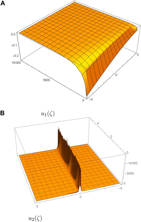
FIGURE 1. Three-dimensional plots of u1(ζ) and u2(ζ) in case 1 for η=0.5, w=1, ρ=1, s=1, l=1, L=1.

Case 2.

$a_0=\frac{9{\rho }^2}{25sw},a_1=-\frac{12l\rho }{5w},a_2=-\frac{12l^{2}s}{w},k=-\frac{6l{\rho }^2}{25Ls},\sigma =-\frac{{\rho }^2}{100l^2{s}^2},$

which produces

$u_3\left(\zeta \right)=\frac{9{\rho }^2}{25sw}+\frac{6{\rho }^2}{25sw}\tanh \frac{\rho }{10ls}\zeta -\frac{3{\rho }^2}{25ws}{\tanh }^2\frac{\rho }{10ls}\zeta ,\tau <0,(25)$

$u_4\left(\zeta \right)=\frac{9{\rho }^2}{25sw}+\frac{6{\rho }^2}{25sw}\coth \frac{\rho }{10ls}\zeta -\frac{3{\rho }^2}{25ws}{\coth }^2\frac{\rho }{10ls}\zeta ,\tau <0,(26)$

where $\zeta =lx+\frac{k{t}^{\eta }}{\mathrm{\Gamma }(\alpha +1)}$, l is an arbitrary constant, and l ≠ 0.

Figure 2 shows the 3D plots of the obtained solutions of the KdVB equation in case 2 for η = 0.5, w = 1, ρ = 1, s = 1, l = 1, and L = 1.

FIGURE 2

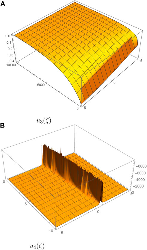
FIGURE 2. Three-dimensional plots of u3(ζ) and u4(ζ) in case 2 with η=0.5, w=1, ρ=1, s=1, l=1, L=1.

4.2 Solving process for the fractional approximate long water wave equation

Equation 2 is transformed into the following ODEs by applying the fractional complex transformation Li and He [26] and He et al. [45]:

$\begin{array}{cc}\hfill & u\left(x,t\right)=u\left(\zeta \right),v\left(x,t\right)=v\left(\zeta \right),\hfill \\ \hfill & \zeta =\frac{l{x}^{\eta }}{\mathrm{\Gamma }\left(\eta +1\right)}+\frac{k{t}^{\eta }}{\mathrm{\Gamma }\left(\eta +1\right)}.\hfill \end{array}(27)$

Then, the following expressions are obtained:

$\begin{array}{cc}\hfill & kL{u}^{\prime }-luL{u}^{\prime }-lL{v}^{\prime }+a{l}^2{L}^2{u}^{″}=0,\hfill \\ \hfill & kL{v}^{\prime }-lL{\left(uv\right)}^{\prime }-a{l}^2{L}^2{v}^{″}=0.\hfill \end{array}(28)$

We perform the same process as mentioned previously and we obtain

$\begin{array}{cc}\hfill & 2ku-l{u}^2-2lv+2a{l}^{2}L{u}^{\prime }=0,\hfill \\ \hfill & kv-l\left(uv\right)-a{l}^{2}L{v}^{\prime }=0.\hfill \end{array}(29)$

Balancing “v” with “u²″ in the first equality in Eq. 29 and “v′” with “UV” in the second equality in Eq. 29, we find n = 1 and m = 2. Therefore, Eq. 15 can be written as

$\begin{array}{cc}\hfill & u\left(\zeta \right)=a_0+a_1\mathrm{\Phi }\left(\zeta \right),\hfill \\ \hfill & v\left(\zeta \right)=b_0+b_1\mathrm{\Phi }\left(\zeta \right)+b_2{\mathrm{\Phi }}^2\left(\zeta \right).\hfill \end{array}(30)$

Substituting Eq. 16 and 30 into Eq. 29, merging the terms of the same degree of Φ, and making the coefficient of each item in the result equal to zero, we obtain the equations for the unknowns a₀, a₁, b₀, b₁, b₂, a, k, l, L, and τ

$\begin{array}{cc}\hfill & 2a_{0}k-{a_0}^{2}l+2l\left(-b_0+a{a}_{1}lL\tau \right)=0,\hfill \\ \hfill & a_0{a}_{1}l+b_{1}l-a_{1}k=0,\hfill \\ \hfill & {a_1}^2+2b_2-2a{a}_{1}lL=0,\hfill \\ \hfill & -a_0{b}_{0}l+b_{0}k-a{b}_1{l}^{2}L\tau =0,\hfill \\ \hfill & b_{1}k-a_0{b}_{1}l-a_1{b}_{0}l-2a{b}_2{l}^{2}L\tau =0,\hfill \\ \hfill & b_{2}k-a_0{b}_{2}l-a_1{b}_{1}l-a{b}_1{l}^{2}L=0,\hfill \\ \hfill & a_1+2alL=0.\hfill \end{array}(31)$

Solving the equations, we have

$a_0=\frac{k}{l},a_1=-2alL,b_0=\frac{k^2}{l^2},b_1=0,b_2=-4a^2{l}^2{L}^2,\tau =-\frac{k^2}{4a^2{l}^4{L}^2}.(32)$

Finally, from Eqs 17, 27, 30 and 32, we obtain the following generalized hyperbolic function solutions of Eq. 2:

$u_1\left(\zeta \right)=\frac{k}{l}+\frac{k}{l}\tanh \frac{k}{2a{l}^{2}L}\zeta ,\tau <0,(33)$

$v_1\left(\zeta \right)=\frac{k^2}{l^2}-\frac{k^2}{l^2}{\tanh }^2\frac{k}{2a{l}^{2}L}\zeta ,\tau <0,(34)$

and

$u_2\left(\zeta \right)=\frac{k}{l}+\frac{k}{l}\coth \frac{k}{2a{l}^{2}L}\zeta ,\tau <0,(35)$

$v_2\left(\zeta \right)=\frac{k^2}{l^2}-\frac{k^2}{l^2}{\coth }^2\frac{k}{2a{l}^{2}L}\zeta ,\tau <0,(36)$

where $\zeta =\frac{l{x}^{\eta }}{\mathrm{\Gamma }(\eta +1)}+\frac{k{t}^{\eta }}{\mathrm{\Gamma }(\eta +1)}$, l and k are arbitrary constants, and l, k ≠ 0.

Figure 3 shows the 3D plots of the obtained solutions of Eq. 2 for η = 0.5, a = 1, l = 1, k = 1, and L = 1.

FIGURE 3

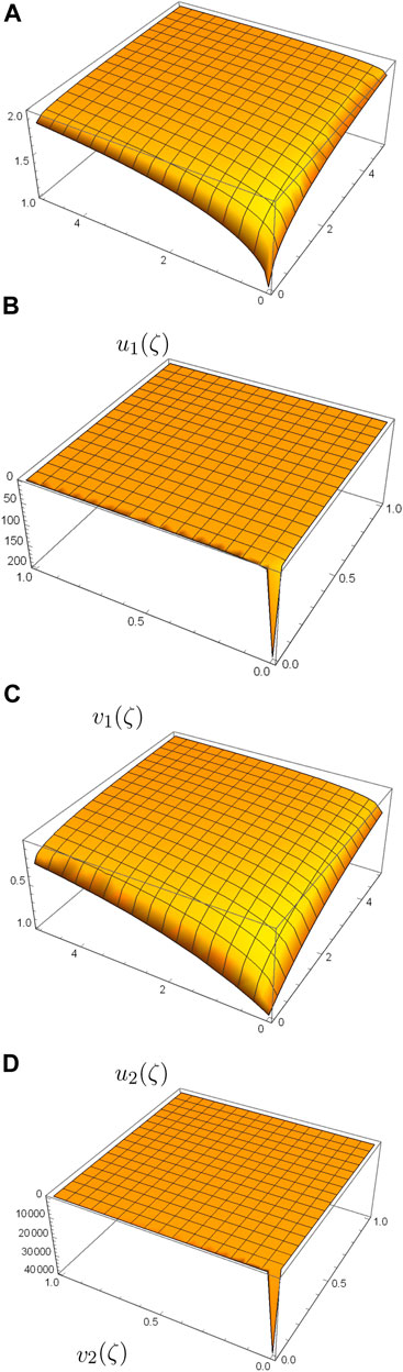
FIGURE 3. Three-dimensional plots of u1(ζ), v1(ζ)and u2(ζ), v2(ζ) of Eq. 2 for η=0.5, a=1, l=1, k=1, L=1.

5 Conclusion

In this paper, some attractive properties of the fractional solitons are elucidated through two examples, and this paper proposes a total new concept on the fractional soliton theory and gives a rigorous mathematical tool to gain deep insights into the physical properties of the fractional solitary solutions, which are practically applicable in many fields. Additionally, this paper also reveals the simplicity, comprehensibility, and effectiveness of the modified extended tanh-function method.

We anticipate that this paper offers a flood of opportunities for finding new physical phenomena of the fractional solitons, and this paper can be used as a good paradigm for future research.

Data availability statement

The original contributions presented in the study are included in the article/supplementary material; further inquiries can be directed to the corresponding author.

Author contributions

All authors listed have made a substantial, direct, and intellectual contribution to the work and approved it for publication.

Funding

This work is supported by the Shaanxi Provincial Education Department (No. 21JK0735) and the National Natural Science Foundation of China (No. 12201485).

Conflict of interest

The authors declare that the research was conducted in the absence of any commercial or financial relationships that could be construed as a potential conflict of interest.

Publisher’s note

All claims expressed in this article are solely those of the authors and do not necessarily represent those of their affiliated organizations, or those of the publisher, the editors, and the reviewers. Any product that may be evaluated in this article, or claim that may be made by its manufacturer, is not guaranteed or endorsed by the publisher.

References

1. Tian Y, Liu J. Direct algebraic method for solving fractional fokas equation. Therm Sci (2021) 25:2235–44. doi:10.2298/TSCI200306111T

CrossRef Full Text | Google Scholar

2. Sun HG, Chen W, Wei H, Chen YQ. A comparative study of constant-order and variable-order fractional models in characterizing memory property of systems. Eur Phys J Spec Top (2011) 193:185–92. doi:10.1140/epjst/e2011-01390-6

CrossRef Full Text | Google Scholar

3. He JH, Hou WF, He CH, Saeed T, Hayat T. Variational approach to fractal solitary waves. Fractals (2021) 29:1–5. doi:10.1142/S0218348X21501991

CrossRef Full Text | Google Scholar

4. He JH, Na Q, He CH. Solitary waves travelling along an unsmooth boundary. Results Phys (2021) 24:104104. doi:10.1016/j.rinp.2021.104104

CrossRef Full Text | Google Scholar

5. Qian MY, He JH. Two-scale thermal science for modern life–making the impossible possible. Therm Sci (2022) 26:2409–12. doi:10.2298/TSCI2203409Q

CrossRef Full Text | Google Scholar

6. Anjum N, Ain QT, Li XX. Two-scale mathematical model for tsunami wave. GEM - Int J Geomathematics (2021) 12:10. doi:10.1007/s13137-021-00177-z

CrossRef Full Text | Google Scholar

7. Çerdik YH. New analytic solutions of the space-time fractional broer–kaup and approximate long water wave equations. J Ocean Eng Sci (2018) 3:295–302. doi:10.1016/j.joes.2018.10.004

CrossRef Full Text | Google Scholar

8. Ling WW, Wu PX. A fractal variational theory of the broer-kaup system in shallow water waves. Therm Sci (2021) 25:2051–6. doi:10.2298/TSCI180510087L

CrossRef Full Text | Google Scholar

9. Lu B. The first integral method for some time fractional differential equations. J Math Anal Appl (2012) 395:684–93. doi:10.1016/j.jmaa.2012.05.066

CrossRef Full Text | Google Scholar

10. Alzaidy JF. The fractional sub-equation method and exact analytical solutions for some nonlinear fractional pdes. Am J Math Anal (2013) 1:14–9. doi:10.12691/ajma-1-1-3

CrossRef Full Text | Google Scholar

11. He JH. Homotopy perturbation technique. Comp Methods Appl Mech Eng (1999) 178:257–62. doi:10.1016/S0045-7825(99)00018-3

CrossRef Full Text | Google Scholar

12. He JH. A coupling method of a homotopy technique and a perturbation technique for non-linear problems. Int J Non-Linear Mech (2000) 35:37–43. doi:10.1016/S0020-7462(98)00085-7

CrossRef Full Text | Google Scholar

13. He JH, El-Dib YO. Homotopy perturbation method with three expansions. J Math Chem (2021) 59:1139–50. doi:10.1007/s10910-021-01237-3

CrossRef Full Text | Google Scholar

14. Nadeem M, He JH, Islam A. The homotopy perturbation method for fractional differential equations: Part 1 mohand transform. Int J Numer Methods Heat Fluid Flow (2021) 31:3490–504. doi:10.1108/HFF-11-2020-0703

CrossRef Full Text | Google Scholar

15. Fang JH, Nadeem M, Habib M, Karim S, Wahash H. A new iterative method for the approximate solution of klein-gordon and sine-gordon equations. J Funct Spaces (2022) 1:1–9. doi:10.1155/2022/5365810

CrossRef Full Text | Google Scholar

16. Nadeem M, He JH. The homotopy perturbation method for fractional differential equations: Part 2, two-scale transform. Int J Numer Methods Heat Fluid Flow (2022) 32:559–67. doi:10.1108/HFF-01-2021-0030

CrossRef Full Text | Google Scholar

17. Filobello-Nino U, Vazquez-Leal H, Khan Y, Perez-Sesma A, Diaz-Sanchez A, Jimenez-Fernandez VM, et al. Laplace transform-homotopy perturbation method as a powerful tool to solve nonlinear problems with boundary conditions defined on finite intervals. Comput Appl Math (2015) 34:1–16. doi:10.1007/s40314-013-0073-z

CrossRef Full Text | Google Scholar

18. Li XX, He CH. Homotopy perturbation method coupled with the enhanced perturbation method. J Low Frequency Noise, Vibration Active Control (2019) 38:1399–403. doi:10.1177/1461348418800554

CrossRef Full Text | Google Scholar

19. Anjum N, He JH, Ain QT, Tian D. Li-he’s modified homotopy perturbation method for doubly-clamped electrically actuated microbeams-based microelectromechanical system. Facta Universitatis, Ser Mech Eng (2021) 19:601–12. doi:10.22190/FUME210112025A

CrossRef Full Text | Google Scholar

20. He JH, El-Dib YO. The enhanced homotopy perturbation method for axial vibration of strings. Facta Universitatis, Ser Mech Eng (2021) 19:735–50. doi:10.22190/FUME210125033H

CrossRef Full Text | Google Scholar

21. Duffy BR, Parkes EJ. Travelling solitary wave solutions to a seventh-order generalized kdv equation. Phys Lett A (1996) 214:271–2. doi:10.1016/0375-9601(96)00184-3

CrossRef Full Text | Google Scholar

22. Parkes EJ, Duffy BR. Travelling solitary wave solutions to a compound kdv-burgers equation. Phys Lett A (1997) 229:217–20. doi:10.1016/S0375-9601(97)00193-X

CrossRef Full Text | Google Scholar

23. Fan EG. Extended tanh-function method and its applications to nonlinear equations. Phys Lett A (2000) 277:212–8. doi:10.1016/S0375-9601(00)00725-8

CrossRef Full Text | Google Scholar

24. Elwakil S, El-Labany S, Zahran M, Sabry R. Modified extended tanh-function method for solving nonlinear partial differential equations. Phys Lett A (2002) 299:179–88. doi:10.1016/S0375-9601(02)00669-2

CrossRef Full Text | Google Scholar

25. Elwakil S, El-Labany S, Zahran M, Sabry R. Modified extended tanh-function method and its applications to nonlinear equations. Appl Math Comput (2005) 161:403–12. doi:10.1016/j.amc.2003.12.035

CrossRef Full Text | Google Scholar

26. Li ZB, He JH. Fractional complex transform for fractional differential equations. Math Comput Appl (2010) 15:970–3. doi:10.3390/mca15050970

CrossRef Full Text | Google Scholar

27. Ain QT, He JH, Anjum N, Ali M. The fractional complex transform: A novel approach to the time-fractional schrodinger equation. Fractals (2020) 28:2050141. doi:10.1142/S0218348X20501418

CrossRef Full Text | Google Scholar

28. Anjum N, Ain QT. Application of he’s fractional derivative and fractional complex transform for time fractional camassa-holm equation. Therm Sci (2020) 24:3023–30. doi:10.2298/TSCI190930450A

CrossRef Full Text | Google Scholar

29. Senol M, Tasbozan O, Kurt A. Numerical solutions of fractional burgers’ type equations with conformable derivative. Chin J Phys (2019) 58:75–84. doi:10.1016/j.cjph.2019.01.001

CrossRef Full Text | Google Scholar

30. Johnson RS. A non-linear equation incorporating damping and dispersion. J Fluid Mech (1970) 42:49–60. doi:10.1017/S0022112070001064

CrossRef Full Text | Google Scholar

31. Benney DJ. Long waves on liquid films. J Math Phys (1966) 45:150–5. doi:10.1002/sapm1966451150

CrossRef Full Text | Google Scholar

32. Wang Q. Homotopy perturbation method for fractional kdv-burgers equation. Chaos, Solitons & Fractals (2008) 35:843–50. doi:10.1016/j.chaos.2006.05.074

CrossRef Full Text | Google Scholar

33. Gupta AK, Ray SS. On the solution of time-fractional KdV–Burgers equation using Petrov–Galerkin method for propagation of long wave in shallow water. Chaos, Solitons & Fractals (2018) 116:376–80. doi:10.1016/j.chaos.2018.09.046

CrossRef Full Text | Google Scholar

34. Yan LM. New travelling wave solutions for coupled fractional variant Boussinesq equation and approximate long water wave equation. Int J Numer Methods Heat Fluid Flow (2015) 25:33–40. doi:10.1108/hff-04-2013-0126

CrossRef Full Text | Google Scholar

35. Guner O, Atik H, Kayyrzhanovich AA. New exact solution for space-time fractional differential equations via g′/g-expansion method. Optik - Int J Light Electron Opt (2017) 130:696–701. doi:10.1016/j.ijleo.2016.10.116

CrossRef Full Text | Google Scholar

36. Kaplan M, Akbulut A. Application of two different algorithms to the approximate long water wave equation with conformable fractional derivative. Arab J Basic Appl Sci (2018) 25:77–84. doi:10.1080/25765299.2018.1449348

CrossRef Full Text | Google Scholar

37. Yang XJ. Advanced local fractional calculus and its applications. New York: World Science Publisher (2012).

Google Scholar

38. Habib S, Batool A, Islam A, Nadeem M, He JH. Study of nonlinear hirota-satsuma coupled kdv and coupled mkdv system with time fractional derivative. Fractals (2021) 29:2150108. doi:10.1142/S0218348X21501085

CrossRef Full Text | Google Scholar

39. Jumarie G. Modified riemann-liouville derivative and fractional Taylor series of nondifferentiable functions further results. Comput Math Appl (2006) 51:1367–76. doi:10.1016/j.camwa.2006.02.001

CrossRef Full Text | Google Scholar

40. He JH. A tutorial review on fractal spacetime and fractional calculus. Int J Theor Phys (2014) 53:3698–718. doi:10.1007/s10773-014-2123-8

CrossRef Full Text | Google Scholar

41. He JH. Fractal calculus and its geometrical explanation. Results Phys (2018) 10:272–6. doi:10.1016/j.rinp.2018.06.011

CrossRef Full Text | Google Scholar

42. Ain QT, He JH. On two-scale dimension and its applications. Therm Sci (2019) 23:1707–12. doi:10.2298/TSCI190408138A

CrossRef Full Text | Google Scholar

43. Atangana A, Baleanu D. New fractional derivatives with nonlocal and non-singular kernel: Theory and application to heat transfer model. Therm Sci (2016) 20:763–9. doi:10.2298/TSCI160111018A

CrossRef Full Text | Google Scholar

44. Ain QT, Sathiyaraj T, Nadeem M, Mwanakatwe PK, Kandege Mwanakatwe P. Abc fractional derivative for the alcohol drinking model using two-scale fractal dimension. Complexity (2022) 8531858:1–11. doi:10.1155/2022/8531858

CrossRef Full Text | Google Scholar

45. He JH, Elagan S, Li Z. Geometrical explanation of the fractional complex transform and derivative chain rule for fractional calculus. Phys Lett A (2012) 376:257–9. doi:10.1016/j.physleta.2011.11.030

CrossRef Full Text | Google Scholar