Fuzzy fractional Gardner and Cahn–Hilliard equations with the Atangana–Baleanu operator

This article focuses on the investigation and computation of solutions to fuzzy fractional-order Cahn–Hilliard and Gardner equations. The study hybridizes the fuzzy Gardner and Cahn–Hilliard equation into two equations using hybrid techniques and the concept of a parametric fuzzy number. To explore these equations, a combination of a novel iterative approach and the Shehu transformation is employed. The article presents detailed procedures for computing a series of solutions to the fractional-order Cahn–Hilliard and Gardner problem. The applied techniques not only offer precision, simplicity, and efficacy but also outperform other existing technologies. Additionally, several examples are solved to validate the proposed theoretical solution.

Introduction

In mathematics, fractional calculus is a useful tool for dealing with ambiguity, recognizing emotional or confusing circumstances, and providing more general answers. Physical models of real-world occurrences may contain significant uncertainty due to a variety of variables. It appears that fuzzy sets can be used to replicate the uncertainty caused by imprecision and ambiguity. If data involve uncertainty, we use it in the medical, environmental, economic, physical, and social sciences. Zadeh investigated these concerns when he contributed fuzziness to set theory in 1965. Fractional calculus has risen in popularity over the last 20 years as a result of its numerous applications in practical research [1–4]. In the behavior of the aforementioned system processes, there are numerous examples of fuzzy uncertainty as opposed to stochastic uncertainty. Many authors have focused on the theoretical foundations of fuzzy problems in recent years. Fractional fuzzy differential equations can be used in civil engineering, population models, electro-hydraulics models, and weapon systems, among others. Fractional fuzzy differential equations are also studied in real-world contexts such as medicine [6], practical systems [7], the golden mean [5], gravity, quantum optics [8], and engineering phenomena. Zadeh [9] became familiar with fuzzy set theory for the first time. The idea of a fuzzy number and its use in fuzzy controls [10] and approximation reasoning problems [11] then became the subjects of research. It is challenging to effectively represent a variety of circumstances using real numbers in data analysis. Later, the fundamentals of fuzzy number arithmetic were specified by Mizumoto and Tanaka [12, 13], Dubois and Prade [14, 15], Nahmias [17], and Ralescu [16]. They used a variety of intervals, such as ϱ-levels, 0 < ϱ ≤ 1, [18], to compute the fuzzy number. It contains information on fuzzy differential equations as well as the fundamental concepts of non-crisp sets. Equations of differential generalization are the recommended notions. Numerous academics have shown interest in this novel idea. Applications of fractional-order differential equations in real-world scenarios are significant; they may be found in fields like engineering, chemistry, and physics. The fractional differential equation is a helpful tool for representing non-linear events in scientific and engineering models. In applied mathematics and engineering, partial differential equations (PDEs), particularly non-linear PDEs, have been utilized to simulate a wide range of scientific phenomena.

Fractional differential equations have received an immense attention in the last two decades because of their ability to mimic a wide range of occurrences in a variety of academic domains and practical applications. Many physical applications in engineering and science can be described using fractional differential equations, which are particularly useful for a wide range of physical challenges. Because these equations are represented by fractional linear and non-linear PDEs, fractional differential equations must be solved [19–21]. The most significant processes occurring in the world are described by non-linear equations. Non-linear partial differential equations remain a challenging topic in both applied mathematics and physics, requiring the employment of a variety of methods to arrive at creative approximations or precise solutions [22–25]. Fractional differential equations have been solved using a variety of numerical and approximation methods. There have been several innovative ways for solving fractional differential equations recently, some of which include the following: the iterative Laplace transform method (ILTM) [27], differential transform method (FDTM) [26], Adomain decomposition technique [29], variational iteration transform technique [30], fractional Adomian decomposition method (FADM) [28], natural decomposition technique [32], and fractional homotopy perturbation technique [31]. The primary goal of this article is to use the natural decomposition technique, one of the most efficient approaches, to solve non-linear fractional Cahn–Hilliard and Gardner equations. Natural decomposition methods do not need discretization, linearization, perturbation, or prescriptive assumptions to prevent round-off errors. The KdV and modified KdV equations were combined to create the Gardner equation [33], which is used to explain internal solitary waves in shallow water. In physics, Gardner’s equation is often applied in fields including quantum field theory, fluid physics, and plasma physics [34, 35]. It also covers a variety of wave events in solid and plasma states [36]. We quickly review the fractional Gardner (FG) equation of the form

$D_{\epsilon }^{ß}\nu \left(\wp ,\epsilon \right)+6\left(\nu -{\mathrm{\Upsilon }}^2{\nu }^2\right)\frac{\partial \nu }{\partial \wp }+\frac{\partial {\nu }^3}{\partial {\wp }^3}=0,0<ß\le 1,(1)$

where ϒ is a real constant. The wave function ν(℘, ɛ) has the scaling variables space (℘) and time (ɛ), the terms $\nu \frac{\partial \nu }{\partial \wp }$ and ${\nu }^2\frac{\partial \nu }{\partial \wp }$ represent non-linear wave steepen, and $\frac{\partial {\nu }^3}{\partial {\wp }^3}$ represents the wave dispersive effect.

In 1958, Cahn and Hilliard [37] developed the Cahn–Hilliard equation to represent the phase separation of a binary alloy at the critical temperature. This equation is essential to several outstanding scientific phenomena, such as phase separation, phase-ordering dynamics, and spinodal decomposition. In this context, the fractional Cahn–Hilliard (FCH) equation is expressed as follows:

$D_{\epsilon }^{ß}\nu \left(\psi ,\epsilon \right)-\frac{\partial \nu }{\partial \psi }-6\nu \frac{\partial {\nu }^2}{\partial \psi }-\left(3{\nu }^2-1\right)\frac{{\partial }^2\nu }{\partial {\psi }^2}+\frac{{\partial }^4\nu }{\partial {\psi }^4}=0,0<ß\le 1.(2)$

Several techniques are applied to analyze the Cahn–Hilliard and Gardner equations, such as the Adomian decomposition method [38], modified Kudryashov method [39], reduced differential transform technique [40], residual power series technique [41], and homotopy perturbation method [42].

The article is organized as follows: theBasic definitionsection provides the basic definition of a fractional fuzzy set. Methodology of the iterative transform method is described in the Roadmap of the suggested techniquesection. The Implementation section describes the application of numerical fuzzy problems, which is followed by the conclusion.

Basic definitions

Definition 2.1. If $\varpi :\mathbb{R}\mapsto [\mathrm{0,1}]$ denotes a fuzzy set, it is understood to be a fuzzy set if the following main requirements hold true [43–46]:

1. ϖ is normal (for some ${\eta }_0\in \mathbb{R};\varpi \left({\vartheta }_0\right)=1$);

2. ϖ is upper semi-continuous;

3. $\varpi \left({\vartheta }_1\omega +(1-\omega ){\vartheta }_2\right)\ge \left(\varpi \left({\vartheta }_1\right)\wedge \varpi \left({\vartheta }_2\right)\right)\forall \omega \in [\mathrm{0,1}],{\vartheta }_1,{\vartheta }_2\in {\mathbb{R}}_{,}$, i.e., ϖ is convex;

4. $cl\{\vartheta \in \mathbb{R},\varpi (\vartheta )>0\}$ is compact.

Definition 2.2. The fuzzy number ϖ is a r-level set expressed as [43–46]

${\left[\varpi \right]}^r=\left\{\nu \in \mathbb{R}:\varpi \left(\nu \right)\ge 1\right\},$

where r ∈ [0, 1] and $\nu \in \mathbb{R}$.

Definition 2.3. A fuzzy number’s parameterized variant is represented as $[\underline{\varpi }(r),\bar{\varpi }(r)]$ such that r ∈ [0, 1] fulfills the following assumptions [43–46]:

1. ϖ(r) is left continuous, left continuous at zero, non-decreasing, and over bounded (0,1];

2. ϖ(r) is right continuous, right continuous at zero, non-increasing, and over bounded (0,1];

3. $\underline{\varpi }(r)\le \bar{\varpi }(r)$.

Definition 2.4. Suppose that there are fuzzy set numbers r ∈ [0, 1] and Y [43–46] $\widetilde{{\rho }_1}=\left({\underline{\rho }}_1,\overline{{\rho }_1}\right),\widetilde{{\rho }_2}=\left(\underline{{\rho }_2},\overline{{\rho }_2}\right)$, then the additions, subtractions, and multiplications, consequently, are defined as follows:

1. $\widetilde{{\rho }_1}\oplus \widetilde{{\rho }_2}=\left(\underline{{\rho }_1}(r)+\underline{{\rho }_2}(r),\overline{{\rho }_1}(r)+\overline{{\rho }_2}(r)\right)$;

2. $\widetilde{{\rho }_1}\ominus \widetilde{{\rho }_2}=\left(\overline{{\rho }_1}(r)-\overline{\underline{{\rho }_2}}(r),\overline{{\rho }_1}(r)-\overline{{\rho }_2}(r)\right)$;

3. $\mathrm{Y}\odot \widetilde{{\rho }_1}=\left\{\left(\mathrm{Y}\underline{{\rho }_1},\mathrm{Y}\overline{{\rho }_1}\right)\mathrm{Y}\ge 0,\left(\mathrm{Y}\overline{{\rho }_1},\mathrm{Y}\underline{{\rho }_1}\right)\mathrm{Y}<0\right.$.

Definition 2.5. the fuzzy mappings $\mathrm{\Theta }:\tilde{E}\times \tilde{E}\mapsto \mathbb{R}$ have fuzzy two sets [43–46] $\widetilde{{\rho }_1}=\left(\underline{{\rho }_1},\overline{{\rho }_1}\right),\widetilde{{\rho }_2}=\left(\underline{{\rho }_2},\overline{{\rho }_2}\right)$, then Θ-distances between $\widetilde{{\rho }_1}$ and $\widetilde{{\rho }_2}$ is defined as

$\mathrm{\Theta }\left(\widetilde{{\rho }_1},\widetilde{{\rho }_2}\right)=\underset{r\in \left[\mathrm{0,1}\right]}{\sup }\left[\max \left\{\underline{\mid {\rho }_1}\left(r\right)-\underline{{\rho }_2}\left(r\right)|,|\overline{{\rho }_1}\left(r\right)-\overline{{\rho }_2}\left(r\right)\mid \right\}\right].$

Theorem 2.1. Consider a fuzzy valued function $\mathbf{E}:\mathbb{R}\mapsto \tilde{E}$ such that $\mathbf{E}\left({\gamma }_0;r\right)=\left[\underline{\mathbf{E}}\left({\gamma }_0;r\right)\right.$, $\left.\bar{\mathbf{E}}\left({\gamma }_0;r\right)\right]$ and r ∈ [0, 1]. Then [43–46],

1. $\left({\gamma }_0;r\right)$ and $\mathbf{E}\left({\gamma }_0;r\right)$ are differentiable functions, if E is a (1)-differentiable function and

${\left[{\mathbf{E}}^{\prime }\left({\gamma }_0\right)\right]}^r=\left[{\underline{\mathbf{E}}}^{\prime }\left({\gamma }_0;r\right),{\bar{\mathbf{E}}}^{\prime }\left({\gamma }_0;r\right)\right].$

11. $\underline{\mathbf{E}}\left({\gamma }_0;r\right)$ and $\bar{\mathbf{E}}\left({\gamma }_0;r\right)$ are differentiable functions, if E is a (2)-differentiable function and

${\left[{\mathbf{E}}^{\prime }\left({\gamma }_0\right)\right]}^r=\left[{\bar{\mathbf{E}}}^{\prime }\left({\gamma }_0;r\right),{\underline{\mathbf{E}}}^{\prime }\left({\gamma }_0;r\right)\right].$

Definition 2.6. Assume that a fuzzy mapping ${\nu }_{g\mathcal{H}}^{(r)}={\nu }^{(r)}\in {\mathbb{C}}^F[0,s]\cap {\mathbb{L}}^F[0,s]$. The fuzzy $g\mathcal{H}$-fractional differentiability Caputo of the fuzzy value mappings nu is thus written as [43–46]

$\begin{array}{cc}\hfill \left(g\mathcal{H}{\mathcal{D}}^{ß}\nu \right)\left(\epsilon \right)& ={\mathcal{J}}_{a_1}^{r-ß}\odot \left({\nu }^{\left(r\right)}\right)\left(\gamma \right)\hfill \\ \hfill & =\frac{1}{\mathrm{\Gamma }\left(r-ß\right)}\odot {\int }_{a_1}^{\epsilon }{\left({\epsilon }_{\mathbf{1}}-\vartheta \right)}^{r-ß-1}\odot {\nu }^{\left(r\right)}\left(\vartheta \right)d\vartheta ,ß\in \left(r-1,r\right],r\in \mathbb{N},\epsilon >a_1.\hfill \end{array}$

The parametric values of $\nu =\left[{\underline{\nu }}_r\left(\epsilon \right),{\bar{\nu }}_r\left(\epsilon \right)\right],r\in [\mathrm{0,1}]$ and ɛ₁₀ ∈ (0, s), and Caputo fractional differential in the presence of fuzzy are expressed as

${\left[{\mathcal{D}}_{\left(i\right)-g\mathcal{H}}^{ß}\nu \left({\epsilon }_{10}\right)\right]}_r=\left[{\mathcal{D}}_{\left(i\right)-g\mathcal{H}}^{ß}\underline{\nu }\left({\epsilon }_{10}\right),{\mathcal{D}}_{\left(i\right)-g\mathcal{H}}^{\theta }\bar{\nu }\left({\epsilon }_{10}\right)\right],r\in \left[\mathrm{0,1}\right],$

where r = [r]

$\begin{array}{cc}\hfill \left[{\mathcal{D}}_{\left(i\right)-g\mathcal{H}}^{ß}\underline{\nu }\left({\epsilon }_{10}\right)\right]& =\frac{1}{\mathrm{\Gamma }\left(r-ß\right)}{\left[{\int }_0^{\epsilon }{\left(\epsilon -\mathbf{x}\right)}^{r-ß-1}\frac{d^r}{d{\mathbf{x}}^r}{\underline{\nu }}_{\left(i\right)-g\mathcal{H}}\left(\mathbf{x}\right)d\mathbf{x}\right]}_{\epsilon ={\epsilon }_{10}},\hfill \\ \hfill \left[{\mathcal{D}}_{\left(i\right)-g\mathcal{H}}^{\theta }\bar{\nu }\left({\epsilon }_{10}\right)\right]& =\frac{1}{\mathrm{\Gamma }\left(r-ß\right)}{\left[{\int }_0^{t_1}{\left(\epsilon -\mathbf{x}\right)}^{r-ß-1}\frac{d^r}{d{\mathbf{x}}^r}{\bar{\nu }}_{\left(i\right)-g\mathcal{H}}\left(\mathbf{x}\right)d\mathbf{x}\right]}_{\epsilon ={\epsilon }_{10}}.\hfill \end{array}$

Definition 2.7. Suppose that fuzzy mappings $\tilde{\nu }\left(\epsilon \right)\in {\tilde{\mathbb{H}}}^1(0,T)$ and ß ∈ [0, 1], then the fuzzy $g\mathcal{H}$-fractional differentiability Atangana–Baleanu of fuzzy value mappings is expressed as

$\left(g\mathcal{H}{\mathcal{D}}^{ß}\nu \right)\left(\epsilon \right)=\frac{\mathbb{B}\left(ß\right)}{1-ß}\odot \left[{\int }_0^{t_1}{\underline{\nu }}^{\prime }\left(\mathbf{x}\right)\odot E_{\text{ß}}\left[\frac{-ß{\left(\epsilon -\mathbf{x}\right)}^{ß}}{1-ß}\right]d\mathbf{x}\right].$

Thus, the parameterized formulation of $\nu =\left[{\underline{\nu }}_r\left(\epsilon \right),{\bar{\nu }}_r\left(\epsilon \right)\right],r\in [\mathrm{0,1}]$ and ɛ₀ ∈ (0, s), and the fuzzy Atangana–Baleanu operator is defined by

$\left[{}^{ABC}\mathcal{D}_{\left(i\right)-g\mathcal{H}}^{ß}\tilde{\nu }\left({\epsilon }_0;r\right)\right]=\left[{}^{ABC}\mathcal{D}_{\left(i\right)-g\mathcal{H}}^{ß}\underline{\nu }\left({\epsilon }_0;r\right),{}^{ABC}\mathcal{D}_{\left(i\right)-g\mathcal{H}}^{\theta }\nu \left({\epsilon }_0;r\right)\right],r\in \left[\mathrm{0,1}\right],$

where

$\begin{array}{cc}\hfill & {}^{ABC}\mathcal{D}_{\left(i\right)-g\mathcal{H}}^{\theta }\underline{\nu }\left({\epsilon }_0;r\right)=\frac{\mathbb{B}\left(ß\right)}{1-ß}{\left[{\int }_0^{t_1}{\underline{\nu }}_{\left(i\right)-g\mathcal{H}}^{\prime }\left(\mathbf{x}\right)E_{\theta }\left[\frac{-ß{\left(\epsilon -\mathbf{x}\right)}^{\theta }}{1-ß}\right]d\mathbf{x}\right]}_{\epsilon ={\epsilon }_0},\hfill \\ \hfill & {}^{ABC}\mathcal{D}_{\left(i\right)-g\mathcal{H}}^{\theta }\bar{\nu }\left({\epsilon }_0;r\right)=\frac{\mathbb{B}\left(ß\right)}{1-ß}{\left[{\int }_0^{t_1}{\bar{\nu }}_{\left(i\right)-g\mathcal{H}}^{\prime }\left(\mathbf{x}\right)E_{\theta }\left[\frac{-ß{\left(\epsilon -\mathbf{x}\right)}^{\theta }}{1-ß}\right]d\mathbf{x}\right]}_{\epsilon ={\epsilon }_0},\hfill \end{array}$

where $\mathbb{B}(ß)$ represents the function of normalization which is equal to 1 when ß is supposed to be 0 and 1. Moreover, we assume that form (i) $-g\mathcal{H}$ exists. Now, there is no requirement to consider the differentiability of (ii) $-g\mathcal{H}$.

Definition 2.8. Suggest a continuous real-value mapping Ψ, and there is an inappropriate Riemann fuzzy integrable mappings $\exp \left(\frac{-\omega }{\sigma }\right)\odot \tilde{\nu }\left(\epsilon \right)$ on [0, + ∞). Then, the integral $\int 0^{+\infty }\exp \left(-\frac{\omega }{\sigma }\right)\odot \tilde{\nu }\left(\epsilon \right)d\epsilon$ is recognized to be the Shehu fuzzy transformation, and it is noted over the set of mapping [43–46]as follows:

$\mathcal{S}=\left\{\tilde{\nu }\left(\mathit{g}\right):\exists \mathcal{A},p_1,p_2>0,\left|\tilde{\nu }\left(\epsilon \right)\right|<\mathcal{A}\exp \left(\frac{\left|\epsilon \right|}{{\psi }_j}\right),\text{\hspace{0.17em}if\hspace{0.17em}}\epsilon \in {\left(-1\right)}^{ȷ}\times \left[0,+\infty \right)\right\},$

as

$\mathbf{S}\left[\tilde{\nu }\left(\epsilon \right)\right]=\mathcal{S}\left(\omega ,\sigma \right)={\int }_0^{+\infty }\exp \left(\frac{-\omega }{\sigma }\epsilon \right)\odot \tilde{\nu }\left(\epsilon \right)d\epsilon ,\omega ,\sigma >0.$

Remark 1

In Equation 14, $\tilde{\nu }$ satisfies the expectation of the reducing diameter $\underline{\nu }$, diameter $\bar{\nu }$ of a mapping of fuzzy ν. If σ = 1, then fuzzy Shehu transform is reduced to * Laplace transform [43–46].

${\int }_0^{+\infty }\exp \left(\frac{-\omega }{\sigma }\epsilon \right)\odot \tilde{\nu }\left(\epsilon \right)d\epsilon =\left({\int }_0^{+\infty }\exp \left(\frac{-\omega }{\sigma }\epsilon \right)\underline{\nu }\left(\epsilon ;r\right)d\epsilon ,{\int }_0^{+\infty }\exp \left(\frac{-\omega }{\sigma }\epsilon \right)\bar{\nu }\left(\epsilon ;r\right)d\epsilon )\right).$

Moreover, by analyzing the traditional Shehu transformation [43–46], we achieve

$\mathbb{S}\left[\underline{\nu }\left(\epsilon ;r\right)\right]={\int }_0^{+\infty }\exp \left(\frac{-\omega }{\sigma }\epsilon \right)\underline{\nu }\left(\epsilon ;r\right)d\epsilon ,$

and

$\mathbb{S}\left[\bar{\nu }\left(\epsilon ;r\right)\right]={\int }_0^{+\infty }\exp \left(\frac{-\omega }{\sigma }\epsilon \right)\bar{\nu }\left(\epsilon ;r\right)d\epsilon .$

The aforementioned expression can then be expressed as

$\begin{array}{cc}\hfill \mathbf{S}\left[\tilde{\nu }\left(\epsilon \right)\right]& =\left(\mathbb{S}\left[\underline{\nu }\left(\epsilon ;r\right)\right],\mathbb{S}\left[\bar{\nu }\left(\epsilon ;r\right)\right]\right)\hfill \\ \hfill & =\left(\underline{\mathcal{S}}\left(\omega ,\sigma \right),\bar{\mathcal{S}}\left(\omega ,\sigma \right)\right).\hfill \end{array}$

Then, we shall define the Caputo generalized Hukuhara derivative’s fuzzy Shehu transformation as ${}_{g\mathcal{H}}{}^c\mathcal{D}_{\epsilon }^{\ominus }\nu \left(\epsilon \right)$.

Definition 2.9. Suppose there is a fuzzy integrable value mapping ${}_{g\mathcal{H}}{}^c\mathcal{D}_{\epsilon }^{ß}\tilde{\nu }\left(\epsilon \right)$, and $\nu \left(\epsilon \right)$ is the primitive of ${}_{g\mathcal{H}}{}^c\mathcal{D}_{\epsilon }^{ß}\tilde{\nu }\left(\epsilon \right)$ on [0, + ∞), then the CFD of order ß is expressed as [43–46]

$\mathbf{S}\left[{}_{g\mathcal{H}}{}^c\mathcal{D}_{\epsilon }^{ß}\tilde{\nu }\left(\epsilon \right)\right]={\left(\frac{\omega }{\sigma }\right)}^{ß}\odot \mathbf{S}\left[\tilde{\nu }\left(\epsilon \right)\right]\ominus {\displaystyle \sum _{ȷ=0}^{r-1}}{\left(\frac{\omega }{\sigma }\right)}^{ß-ȷ-1}\odot {\tilde{\nu }}^{\left(ȷ\right)}\left(0\right),ß\in \left(r-1,r\right],$

$\begin{array}{cc}\hfill & {\left(\frac{\omega }{\sigma }\right)}^{ß}\odot \mathbf{S}\left[\tilde{\nu }\left(\epsilon \right)\right]\ominus {\displaystyle \sum _{ȷ=0}^{r-1}}{\left(\frac{\omega }{\sigma }\right)}^{ß-ȷ-1}\odot {\tilde{f}}^{\left(ȷ\right)}\left(0\right)\hfill \\ \hfill & =\left({\left(\frac{\omega }{\sigma }\right)}^{ß}\mathbf{S}\left[\underline{\nu }\left(\epsilon ;r\right)\right]-{\displaystyle \sum _{ȷ=0}^{r-1}}{\left(\frac{\omega }{\sigma }\right)}^{ß-ȷ-1}\odot {\underline{\nu }}^{\left(ȷ\right)}\left(0;r\right),\right.\hfill \\ \hfill & \left.{\left(\frac{\omega }{\sigma }\right)}^{ß}\mathbf{S}\left[\bar{\nu }\left(\epsilon ;r\right)\right]-{\displaystyle \sum _{ȷ=0}^{r-1}}{\left(\frac{\omega }{\sigma }\right)}^{ß-ȷ-1}{\bar{\nu }}^{\left(ȷ\right)}\left(0;r\right)\right).\hfill \end{array}$

Bokhari et al. defined the ABC operator’s fractional derivative in terms of the Shehu transform. Additionally, we extend the concept of fuzzy ABC fractional derivative in the context of a fuzzy Shehu transform as follows:

Definition 2.10. Consider $\nu \in {\mathbb{C}}^F[0,s]\cap {\mathbb{L}}^F[0,s]$ such that $\tilde{\nu }\left(\epsilon \right)=\left[\underline{\nu }\left(\epsilon ,r\right),\bar{\nu }\left(\epsilon ,r\right)\right]$, r ∈ [0, 1]; then, the Shehu transformation of the fuzzy ABC of order ß ∈ [0, 1] is defined as follows:

$\mathbf{S}\left[g\mathcal{H}{\mathcal{D}}_{\epsilon }^{ß}\tilde{\nu }\left(\epsilon \right)\right]=\frac{\mathbb{B}\left(ß\right)}{1-ß+ß{\left(\frac{\sigma }{\omega }\right)}^{ß}}\odot \left(\tilde{\mathbf{V}}\left(\sigma ,\omega \right)\ominus \frac{\sigma }{\omega }\tilde{\nu }\left(0\right)\right).$

Moreover, by applying the fact of Salahshour et al. [45], we obtain

$\begin{array}{cc}\hfill & \frac{\mathbb{B}\left(ß\right)}{1-ß+ß{\left(\frac{\sigma }{\tilde{\omega }}\right)}^{ß}}\odot \left(\tilde{\mathbf{V}}\left(\sigma ,\omega \right)\ominus \frac{\omega }{\sigma }\tilde{\nu }\left(0\right)\right)\hfill \\ \hfill & =(\frac{\mathbb{B}\left(ß\right)}{1-ß+ß{\left(\frac{\sigma }{\tilde{\omega }}\right)}^{ß}}\left(\underline{\mathbf{V}}\left(\sigma ,\omega ;r\right)-\frac{\sigma }{\omega }\nu \left(0;r\right)\right),\frac{\mathbb{B}\left(ß\right)}{1-ß+ß{\left(\frac{\sigma }{\psi }\right)}^{\theta }}\left(\bar{\mathbf{V}}\left(\sigma ,\omega ;r\right)-\frac{\sigma }{\tilde{\omega }}\bar{\nu }\left(0;r\right)\right)).\hfill \end{array}$

Road map of the suggested technique

Consider the fractional fuzzy partial differential equation

$\mathcal{S}\left[{}^{ABC}D_{\epsilon }^{ß}\tilde{\nu }\left(\psi ,\epsilon \right)\right]=\mathcal{S}\left[D_{\psi }^2\tilde{\nu }\left(\psi ,\epsilon \right)+D_{\psi }^3\tilde{\nu }\left(\psi ,\epsilon \right)+\tilde{k}\left(r\right)\mathcal{F}\left(\psi ,\epsilon \right)\right],(3)$

where ß ∈ (0, 1]; therefore, the Shehu transform of Equation 3 is

$\begin{array}{ll}\hfill & \frac{\mathbb{B}\left(ß\right)}{1-ß+ß{\left(\frac{\sigma }{\omega }\right)}^{ß}}\mathcal{S}\left[\tilde{\nu }\left(\psi ,\epsilon \right)\right]-\frac{\mathbb{B}\left(ß\right)}{1-ß+ß{\left(\frac{\sigma }{\omega }\right)}^{ß}}\left(\frac{v}{\omega }\right)\tilde{\nu }\left(\psi ,\xi ,0\right)\hfill \\ \hfill & =\mathcal{S}\left[D_{\psi }^2\tilde{\nu }\left(\psi ,\epsilon \right)+D_{\psi }^3\tilde{\nu }\left(\psi ,\epsilon \right)+\tilde{k}\left(r\right)\mathcal{F}\left(\psi ,\epsilon \right)\right].\hfill \end{array}$

On using the initial condition, we obtain

$\mathcal{S}\left[\tilde{\nu }\left(\psi ,\epsilon \right)\right]=\frac{g\left(\psi ,\xi \right)}{\omega }+\frac{1-ß+ß{\left(\frac{\sigma }{\omega }\right)}^{ß}}{\mathbb{B}\left(ß\right)}\mathcal{S}\left[D_{\psi }^2\tilde{\nu }\left(\psi ,\epsilon \right)+D_{\psi }^3\tilde{\nu }\left(\psi ,\epsilon \right)+\tilde{k}\left(r\right)\mathcal{F}\left(\psi ,\epsilon \right)\right].(4)$

Decomposing the solution as $\tilde{\nu }(\psi ,\epsilon )={\sum }_{n=0}^{\infty }{\tilde{\nu }}_n(\psi ,\epsilon )$, then (4) implies

$\begin{array}{cc}\hfill \mathcal{S}{\displaystyle \sum _{n=0}^{\infty }}{\tilde{\nu }}_n\left(\psi ,\epsilon \right)& =\frac{g\left(\psi ,\xi \right)}{\omega }+\frac{1-ß+ß{\left(\frac{\sigma }{\omega }\right)}^{ß}}{\mathbb{B}\left(ß\right)}\mathcal{S}\left[D_{\psi }^2{\displaystyle \sum _{n=0}^{\infty }}{\tilde{\nu }}_n\left(\psi ,\epsilon \right)\right.\hfill \\ \hfill & +\left.D_{\psi }^3{\displaystyle \sum _{n=0}^{\infty }}{\tilde{\nu }}_n\left(\psi ,\epsilon \right)+\tilde{k}\left(r\right)\mathcal{F}\left(\psi ,\epsilon \right)\right].\hfill \end{array}(5)$

Taking parts of the solution by the choice of comparison, we obtain

$\begin{array}{cc}\hfill \mathcal{S}\left[{\tilde{\nu }}_0\left(\psi ,\epsilon \right)\right]& =\frac{g\left(\psi ,\xi \right)}{\omega }+\frac{1-ß+ß{\left(\frac{\sigma }{\omega }\right)}^{ß}}{\mathbb{B}\left(ß\right)}\mathcal{S}\left[\tilde{k}\left(r\right)\mathcal{F}\left(\psi ,\epsilon \right)\right].\hfill \\ \hfill \mathcal{S}\left[{\tilde{\nu }}_1\left(\psi ,\epsilon \right)\right]& =\frac{1-ß+ß{\left(\frac{\sigma }{\omega }\right)}^{ß}}{\mathbb{B}\left(ß\right)}\mathcal{S}\left[D_{\psi }^2{\tilde{\nu }}_0\left(\psi ,\epsilon \right)+D_{\psi }^3{\tilde{\nu }}_0\left(\psi ,\epsilon \right)\right].\hfill \\ \hfill \mathcal{S}\left[{\tilde{\nu }}_2\left(\psi ,\epsilon \right)\right]& =\frac{1-ß+ß{\left(\frac{\sigma }{\omega }\right)}^{ß}}{\mathbb{B}\left(ß\right)}\mathcal{S}\left[D_{\psi }^2{\tilde{\nu }}_1\left(\psi ,\epsilon \right)+D_{\psi }^3{\tilde{\nu }}_1\left(\psi ,\epsilon \right)\right].\hfill \\ \hfill & ⋮\hfill \\ \hfill \mathcal{S}\left[{\tilde{\nu }}_{n+1}\left(\psi ,\epsilon \right)\right]& =\frac{1-ß+ß{\left(\frac{\sigma }{\omega }\right)}^{ß}}{\mathbb{B}\left(ß\right)}\mathcal{S}\left[D_{\psi }^2{\tilde{\nu }}_n\left(\psi ,\epsilon \right)+D_{\psi }^3{\tilde{\nu }}_n\left(\psi ,\epsilon \right)\right].\hfill \end{array}(6)$

Taking the inverse Shehu transform, we obtain

$\begin{array}{cc}\hfill {\underline{\nu }}_0\left(\psi ,\epsilon \right)& =g\left(\psi ,\xi \right)+{\mathcal{S}}^{-1}\left[\frac{1-ß+ß{\left(\frac{\sigma }{\omega }\right)}^{ß}}{\mathbb{B}\left(ß\right)}\mathcal{S}\left[\underline{k}\left(r\right)\mathcal{F}\left(\psi ,\epsilon \right)\right]\right],\hfill \\ \hfill {\bar{\nu }}_0\left(\psi ,\epsilon \right)& =g\left(\psi ,\xi \right)+{\mathcal{S}}^{-1}\left[\frac{1-ß+ß{\left(\frac{\sigma }{\omega }\right)}^{ß}}{\mathbb{B}\left(ß\right)}\mathcal{S}\left[\bar{k}\left(r\right)\mathcal{F}\left(\psi ,\epsilon \right)\right]\right],\hfill \\ \hfill {\underline{\nu }}_1\left(\psi ,\epsilon \right)& ={\mathcal{S}}^{-1}\left[\frac{1-ß+ß{\left(\frac{\sigma }{\omega }\right)}^{ß}}{\mathbb{B}\left(ß\right)}\mathcal{S}\left[D_{\psi }^2{\underline{\nu }}_0\left(\psi ,\epsilon \right)+D_{\psi }^3{\underline{\nu }}_0\left(\psi ,\epsilon \right)\right]\right],\hfill \\ \hfill {\bar{\nu }}_1\left(\psi ,\epsilon \right)& ={\mathcal{S}}^{-1}\left[\frac{1-ß+ß{\left(\frac{\sigma }{\omega }\right)}^{ß}}{\mathbb{B}\left(ß\right)}\mathcal{S}\left[D_{\psi }^2{\bar{\nu }}_0\left(\psi ,\epsilon \right)+D_{\psi }^3{\bar{\nu }}_0\left(\psi ,\epsilon \right)\right]\right],\hfill \\ \hfill {\underline{\nu }}_2\left(\psi ,\epsilon \right)& ={\mathcal{S}}^{-1}\left[\frac{1-ß+ß{\left(\frac{\sigma }{\omega }\right)}^{ß}}{\mathbb{B}\left(ß\right)}\mathcal{S}\left[D_{\psi }^2{\underline{\nu }}_1\left(\psi ,\epsilon \right)+D_{\psi }^3{\underline{\nu }}_1\left(\psi ,\epsilon \right)\right]\right],\hfill \\ \hfill {\bar{\nu }}_2\left(\psi ,\epsilon \right)& ={\mathcal{S}}^{-1}\left[\frac{1-ß+ß{\left(\frac{\sigma }{\omega }\right)}^{ß}}{\mathbb{B}\left(ß\right)}\mathcal{S}\left[D_{\psi }^2{\bar{\nu }}_1\left(\psi ,\epsilon \right)+D_{\psi }^3{\bar{\nu }}_1\left(\psi ,\epsilon \right)\right]\right],\hfill \\ \hfill & ⋮\hfill \\ \hfill {\underline{\nu }}_{n+1}\left(\psi ,\epsilon \right)& ={\mathcal{S}}^{-1}\left[\frac{1-ß+ß{\left(\frac{\sigma }{\omega }\right)}^{ß}}{\mathbb{B}\left(ß\right)}\mathcal{S}\left[D_{\psi }^2{\underline{\nu }}_n\left(\psi ,\epsilon \right)+D_{\psi }^3{\underline{\nu }}_n\left(\psi ,\epsilon \right)\right]\right],\hfill \\ \hfill {\bar{\nu }}_{n+1}\left(\psi ,\epsilon \right)& ={\mathcal{S}}^{-1}\left[\frac{1-ß+ß{\left(\frac{\sigma }{\omega }\right)}^{ß}}{\mathbb{B}\left(ß\right)}\mathcal{S}\left[D_{\psi }^2{\bar{\nu }}_n\left(\psi ,\epsilon \right)+D_{\psi }^3{\bar{\nu }}_n\left(\psi ,\epsilon \right)\right]\right].\hfill \end{array}(7)$

Thus, the solution becomes

$\begin{array}{cc}\hfill \underline{\nu }\left(\psi ,\epsilon \right)& ={\underline{\nu }}_0\left(\psi ,\epsilon \right)+{\underline{\nu }}_1\left(\psi ,\epsilon \right)+{\underline{\nu }}_2\left(\psi ,\epsilon \right)+\cdots ,\hfill \\ \hfill \bar{\nu }\left(\psi ,\epsilon \right)& ={\bar{\nu }}_0\left(\psi ,\epsilon \right)+{\bar{\nu }}_1\left(\psi ,\epsilon \right)+{\bar{\nu }}_2\left(\psi ,\epsilon \right)+\cdots .\hfill \end{array}(8)$

Equation 8 is the solution in series form.

Implementation

Example 4.1. Consider the fractional fuzzy Gardner equation as follows:

${}^{ABC}D_{\epsilon }^{ß}\tilde{\nu }\left(\psi ,\epsilon \right)+6\left(\tilde{\nu }\left(\psi ,\epsilon \right)-{\mathrm{\Upsilon }}^2{\tilde{\nu }}^2\left(\psi ,\epsilon \right)\right)\frac{\partial \tilde{\nu }\left(\psi ,\epsilon \right)}{\partial \psi }+\frac{\partial {\tilde{\nu }}^3\left(\psi ,\epsilon \right)}{\partial {\psi }^3}=0,0<ß\le 1,(9)$

with the fuzzy initial condition

$\tilde{\nu }\left(\psi ,0\right)=\tilde{k}\left(\frac{1}{2}+\frac{1}{2}\tanh \left(\frac{\psi }{2}\right)\right).(10)$

Applying the proposed Equation 7, we achieve

$\begin{array}{cc}\hfill {\underline{\nu }}_0\left(\psi ,\epsilon \right)& =\underline{k}\left(r\right)\left(\frac{1}{2}+\frac{1}{2}\tanh \left(\frac{\psi }{2}\right)\right),\hfill \\ \hfill {\bar{\nu }}_0\left(\psi ,\epsilon \right)& =\bar{k}\left(r\right)\left(\frac{1}{2}+\frac{1}{2}\tanh \left(\frac{\psi }{2}\right)\right),\hfill \\ \hfill {\underline{\nu }}_1\left(\psi ,\epsilon \right)& =\underline{k}\left(r\right)\frac{{\mathrm{sech}}^2\left(\frac{\psi }{2}\right)\left(-1+\left(-4+3{\mathrm{\Upsilon }}^2\right)\cosh \left(\psi \right)+3\left(-1+{\mathrm{\Upsilon }}^2\right)\sinh \left(\psi \right)\right)}{8}\hfill \\ \hfill & \times \frac{1}{\mathbb{B}\left(ß\right)}\left\{\frac{ß{\epsilon }^{ß}}{\mathrm{\Gamma }\left(ß+1\right)}+\left(1-ß\right)\right\},\hfill \\ \hfill {\bar{\nu }}_1\left(\psi ,\epsilon \right)& =\bar{k}\left(r\right)\frac{{\mathrm{sech}}^2\left(\frac{\psi }{2}\right)\left(-1+\left(-4+3{\mathrm{\Upsilon }}^2\right)\cosh \left(\psi \right)+3\left(-1+{\mathrm{\Upsilon }}^2\right)\sinh \left(\psi \right)\right)}{8}\hfill \\ \hfill & \times \frac{1}{\mathbb{B}\left(ß\right)}\left\{\frac{ß{\epsilon }^{ß}}{\mathrm{\Gamma }\left(ß+1\right)}+\left(1-ß\right)\right\},\hfill \end{array}(11)$

$\begin{array}{cc}\hfill {\underline{\nu }}_2\left(\psi ,\epsilon \right)& =\underline{k}\left(r\right)\frac{-{\mathrm{sech}}^7\left(\frac{\psi }{2}\right)}{64}\left(-24\left(-1+{\mathrm{\Upsilon }}^2\right)\cosh \left(\frac{\psi }{2}\right)-6\left(22-37{\mathrm{\Upsilon }}^2+15{\mathrm{\Upsilon }}^4\right)\right.\hfill \\ \hfill & \times \cosh \left(\frac{3\psi }{2}\right)+6\left(4-7{\mathrm{\Upsilon }}^2+3{\mathrm{\Upsilon }}^4\right)\cosh \left(\frac{5\psi }{2}\right)+2\left(103-102{\mathrm{\Upsilon }}^2\right)\sinh \left(\frac{\psi }{2}\right)\hfill \\ \hfill & -3\left(43-74{\mathrm{\Upsilon }}^2+30{\mathrm{\Upsilon }}^4\right)\sinh \left(\frac{3\psi }{2}\right)+\left(25-42{\mathrm{\Upsilon }}^2+18{\mathrm{\Upsilon }}^4\right)\sinh \left.\left(\frac{5\psi }{2}\right)\right)\hfill \\ \hfill & \times \frac{1}{{\mathbb{B}}^2\left(ß\right)}\left\{\frac{{ß}^2{\epsilon }^{2ß}}{\mathrm{\Gamma }\left(2ß+1\right)}+2ß\left(1-ß\right)\frac{{\epsilon }^{ß}}{\mathrm{\Gamma }\left(ß+1\right)}+{\left(1-ß\right)}^2\right\},\hfill \\ \hfill {\bar{\nu }}_2\left(\psi ,\epsilon \right)& =\bar{k}\left(r\right)\frac{-{\mathrm{sech}}^7\left(\frac{\psi }{2}\right)}{64}\left(-24\left(-1+{\mathrm{\Upsilon }}^2\right)\cosh \left(\frac{\psi }{2}\right)-6\left(22-37{\mathrm{\Upsilon }}^2+15{\mathrm{\Upsilon }}^4\right)\right.\hfill \\ \hfill & \times \cosh \left(\frac{3\psi }{2}\right)+6\left(4-7{\mathrm{\Upsilon }}^2+3{\mathrm{\Upsilon }}^4\right)\cosh \left(\frac{5\psi }{2}\right)+2\left(103-102{\mathrm{\Upsilon }}^2\right)\sinh \left(\frac{\psi }{2}\right)\hfill \\ \hfill & -3\left(43-74{\mathrm{\Upsilon }}^2+30{\mathrm{\Upsilon }}^4\right)\sinh \left(\frac{3\psi }{2}\right)+\left(25-42{\mathrm{\Upsilon }}^2+18{\mathrm{\Upsilon }}^4\right)\sinh \left.\left(\frac{5\psi }{2}\right)\right)\hfill \\ \hfill & \times \frac{1}{{\mathbb{B}}^2\left(ß\right)}\left\{\frac{{ß}^2{\epsilon }^{2ß}}{\mathrm{\Gamma }\left(2ß+1\right)}+2ß\left(1-ß\right)\frac{{\epsilon }^{ß}}{\mathrm{\Gamma }\left(ß+1\right)}+{\left(1-ß\right)}^2\right\}.\hfill \end{array}(12)$

The higher terms can also be obtained in a similar manner. Equation 8 provides solution in series form; consequently, we write

$\tilde{\nu }\left(\psi ,\epsilon \right)={\tilde{\nu }}_0\left(\psi ,\epsilon \right)+{\tilde{\nu }}_1\left(\psi ,\epsilon \right)+{\tilde{\nu }}_2\left(\psi ,\epsilon \right)+{\tilde{\nu }}_3\left(\psi ,\epsilon \right)+{\tilde{\nu }}_4\left(\psi ,\epsilon \right)+\cdots ,(13)$

while, in lower and upper portion types, it is, respectively, written as

$\begin{array}{cc}\hfill \underline{\nu }\left(\psi ,\epsilon \right)& ={\underline{\nu }}_0\left(\psi ,\epsilon \right)+{\underline{\nu }}_1\left(\psi ,\epsilon \right)+{\underline{\nu }}_2\left(\psi ,\epsilon \right)+{\underline{\nu }}_3\left(\psi ,\epsilon \right)+{\underline{\nu }}_4\left(\psi ,\epsilon \right)+\cdots ,\hfill \\ \hfill \bar{\nu }\left(\psi ,\epsilon \right)& ={\bar{\nu }}_0\left(\psi ,\epsilon \right)+{\bar{\nu }}_1\left(\psi ,\epsilon \right)+{\bar{\nu }}_2\left(\psi ,\epsilon \right)+{\bar{\nu }}_3\left(\psi ,\epsilon \right)+{\bar{\nu }}_4\left(\psi ,\epsilon \right)+\cdots .\hfill \end{array}(14)$

$\begin{array}{cc}\hfill & \underline{\nu }\left(\psi ,\epsilon \right)=\underline{k}\left(r\right)\left(\frac{1}{2}+\frac{1}{2}\tanh \left(\frac{\psi }{2}\right)\right)+\underline{k}\left(r\right)\frac{{\mathrm{sech}}^2\left(\frac{\psi }{2}\right)\left(-1+\left(-4+3{\mathrm{\Upsilon }}^2\right)\cosh \left(\psi \right)+3\left(-1+{\mathrm{\Upsilon }}^2\right)\sinh \left(\psi \right)\right)}{8}\hfill \\ \hfill & \frac{1}{\mathbb{B}\left(ß\right)}\left\{\frac{ß{\epsilon }^{ß}}{\mathrm{\Gamma }\left(ß+1\right)}+\left(1-ß\right)\right\}+\underline{k}\left(r\right)\frac{-{\mathrm{sech}}^7\left(\frac{\psi }{2}\right)}{64}\left(-24\left(-1+{\mathrm{\Upsilon }}^2\right)\cosh \left(\frac{\psi }{2}\right)-6\left(22-37{\mathrm{\Upsilon }}^2+15{\mathrm{\Upsilon }}^4\right)\cosh \left(\frac{3\psi }{2}\right)\right.\hfill \\ \hfill & +6\left(4-7{\mathrm{\Upsilon }}^2+3{\mathrm{\Upsilon }}^4\right)\cosh \left(\frac{5\psi }{2}\right)+2\left(103-102{\mathrm{\Upsilon }}^2\right)\sinh \left(\frac{\psi }{2}\right)-3\left(43-74{\mathrm{\Upsilon }}^2+30{\mathrm{\Upsilon }}^4\right)\hfill \\ \hfill & \left.\sinh \left(\frac{3\psi }{2}\right)+\left(25-42{\mathrm{\Upsilon }}^2+18{\mathrm{\Upsilon }}^4\right)\sinh \left(\frac{5\psi }{2}\right)\right)\frac{1}{{\mathbb{B}}^2\left(ß\right)}\left\{\frac{{ß}^2{\epsilon }^{2ß}}{\mathrm{\Gamma }\left(2ß+1\right)}+2ß\left(1-ß\right)\frac{{\epsilon }^{ß}}{\mathrm{\Gamma }\left(ß+1\right)}+{\left(1-ß\right)}^2\right\}+\cdots ,\hfill \\ \hfill & \bar{\nu }\left(\psi ,\epsilon \right)=\bar{k}\left(r\right)\left(\frac{1}{2}+\frac{1}{2}\tanh \left(\frac{\psi }{2}\right)\right)+\bar{k}\left(r\right)\frac{{\mathrm{sech}}^2\left(\frac{\psi }{2}\right)\left(-1+\left(-4+3{\mathrm{\Upsilon }}^2\right)\cosh \left(\psi \right)+3\left(-1+{\mathrm{\Upsilon }}^2\right)\sinh \left(\psi \right)\right)}{8}\hfill \\ \hfill & \frac{1}{\mathbb{B}\left(ß\right)}\left\{\frac{ß{\epsilon }^{ß}}{\mathrm{\Gamma }\left(ß+1\right)}+\left(1-ß\right)\right\}+\bar{k}\left(r\right)\frac{-{\mathrm{sech}}^7\left(\frac{\psi }{2}\right)}{64}\left(-24\left(-1+{\mathrm{\Upsilon }}^2\right)\cosh \left(\frac{\psi }{2}\right)-6\left(22-37{\mathrm{\Upsilon }}^2+15{\mathrm{\Upsilon }}^4\right)\cosh \left(\frac{3\psi }{2}\right)\right.\hfill \\ \hfill & +6\left(4-7{\mathrm{\Upsilon }}^2+3{\mathrm{\Upsilon }}^4\right)\cosh \left(\frac{5\psi }{2}\right)+2\left(103-102{\mathrm{\Upsilon }}^2\right)\sinh \left(\frac{\psi }{2}\right)-3\left(43-74{\mathrm{\Upsilon }}^2+30{\mathrm{\Upsilon }}^4\right)\hfill \\ \hfill & \left.\sinh \left(\frac{3\psi }{2}\right)+\left(25-42{\mathrm{\Upsilon }}^2+18{\mathrm{\Upsilon }}^4\right)\sinh \left(\frac{5\psi }{2}\right)\right)\frac{1}{{\mathbb{B}}^2\left(ß\right)}\left\{\frac{{ß}^2{\epsilon }^{2ß}}{\mathrm{\Gamma }\left(2ß+1\right)}+2ß\left(1-ß\right)\frac{{\epsilon }^{ß}}{\mathrm{\Gamma }\left(ß+1\right)}+{\left(1-ß\right)}^2\right\}+\cdots .\hfill \end{array}(15)$

The exact result is given as

$\tilde{\nu }\left(\psi ,\epsilon \right)=\tilde{k}\left(\frac{1}{2}+\frac{1}{2}\tanh \left(\frac{\psi -\epsilon }{2}\right)\right).(16)$

Example 4.2. Consider the fractional fuzzy Cahn–Hilliard equation as follows:

$\begin{array}{ll}\hfill D_{\epsilon }^{ß}\tilde{\nu }\left(\psi ,\epsilon \right)-\frac{\partial \tilde{\nu }\left(\psi ,\epsilon \right)}{\partial \psi }-6\tilde{\nu }\left(\psi ,\epsilon \right)\frac{\partial {\tilde{\nu }}^2\left(\psi ,\epsilon \right)}{\partial \psi }-\left(3{\tilde{\nu }}^2\left(\psi ,\epsilon \right)-1\right)\frac{{\partial }^2\tilde{\nu }\left(\psi ,\epsilon \right)}{\partial {\psi }^2}+\frac{{\partial }^4\tilde{\nu }\left(\psi ,\epsilon \right)}{\partial {\psi }^4}& =0,\hfill \\ \hfill & 0<ß\le 1,\hfill \end{array}(17)$

with the fuzzy initial condition

$\tilde{\nu }\left(\psi ,0\right)=\tilde{k}\tanh \left(\frac{\psi }{\sqrt{2}}\right).(18)$

Applying the system of Equation 7, we achieve

$\begin{array}{cc}\hfill {\underline{\nu }}_0\left(\psi ,\epsilon \right)& =\underline{k}\left(r\right)\tanh \left(\frac{\psi }{\sqrt{2}}\right),\hfill \\ \hfill {\bar{\nu }}_0\left(\psi ,\epsilon \right)& =\bar{k}\left(r\right)\tanh \left(\frac{\psi }{\sqrt{2}}\right),\hfill \\ \hfill {\underline{\nu }}_1\left(\psi ,\epsilon \right)& =\underline{k}\left(r\right){\mathrm{sech}}^2\frac{\left(\frac{\psi }{\sqrt{2}}\right)}{\sqrt{2}}\frac{1}{\mathbb{B}\left(ß\right)}\left\{\frac{ß{\epsilon }^{ß}}{\mathrm{\Gamma }\left(ß+1\right)}+\left(1-ß\right)\right\},\hfill \\ \hfill {\bar{\nu }}_1\left(\psi ,\epsilon \right)& =\bar{k}\left(r\right){\mathrm{sech}}^2\frac{\left(\frac{\psi }{\sqrt{2}}\right)}{\sqrt{2}}\frac{1}{\mathbb{B}\left(ß\right)}\left\{\frac{ß{\epsilon }^{ß}}{\mathrm{\Gamma }\left(ß+1\right)}+\left(1-ß\right)\right\},\hfill \end{array}(19)$

$\begin{array}{cc}\hfill {\underline{\nu }}_2\left(\psi ,\epsilon \right)& =-\underline{k}\left(r\right){\mathrm{sech}}^2\left(\frac{\psi }{\sqrt{2}}\right)\tanh \left(\frac{\psi }{\sqrt{2}}\right)\frac{1}{{\mathbb{B}}^2\left(ß\right)}\hfill \\ \hfill & \times \left\{\frac{{ß}^2{\epsilon }^{2ß}}{\mathrm{\Gamma }\left(2ß+1\right)}+2ß\left(1-ß\right)\frac{{\epsilon }^{ß}}{\mathrm{\Gamma }\left(ß+1\right)}+{\left(1-ß\right)}^2\right\},\hfill \\ \hfill {\bar{\nu }}_2\left(\psi ,\epsilon \right)& =-\bar{k}\left(r\right){\mathrm{sech}}^2\left(\frac{\psi }{\sqrt{2}}\right)\tanh \left(\frac{\psi }{\sqrt{2}}\right)\frac{1}{{\mathbb{B}}^2\left(ß\right)}\hfill \\ \hfill & \times \left\{\frac{{ß}^2{\epsilon }^{2ß}}{\mathrm{\Gamma }\left(2ß+1\right)}+2ß\left(1-ß\right)\frac{{\epsilon }^{ß}}{\mathrm{\Gamma }\left(ß+1\right)}+{\left(1-ß\right)}^2\right\}.\hfill \end{array}(20)$

The higher terms can also be obtained in a similar manner. Equation 8 provides solution in series form; consequently, we write

$\tilde{\nu }\left(\psi ,\epsilon \right)={\tilde{\nu }}_0\left(\psi ,\epsilon \right)+{\tilde{\nu }}_1\left(\psi ,\epsilon \right)+{\tilde{\nu }}_2\left(\psi ,\epsilon \right)+{\tilde{\nu }}_3\left(\psi ,\epsilon \right)+{\tilde{\nu }}_4\left(\psi ,\epsilon \right)+\cdots .(21)$

In the lower and upper portion types, it is, respectively, written as

$\begin{array}{cc}\hfill \underline{\nu }\left(\psi ,\epsilon \right)& ={\underline{\nu }}_0\left(\psi ,\epsilon \right)+{\underline{\nu }}_1\left(\psi ,\epsilon \right)+{\underline{\nu }}_2\left(\psi ,\epsilon \right)+{\underline{\nu }}_3\left(\psi ,\epsilon \right)+{\underline{\nu }}_4\left(\psi ,\epsilon \right)+\cdots ,\hfill \\ \hfill \bar{\nu }\left(\psi ,\epsilon \right)& ={\bar{\nu }}_0\left(\psi ,\epsilon \right)+{\bar{\nu }}_1\left(\psi ,\epsilon \right)+{\bar{\nu }}_2\left(\psi ,\epsilon \right)+{\bar{\nu }}_3\left(\psi ,\epsilon \right)+{\bar{\nu }}_4\left(\psi ,\epsilon \right)+\cdots .\hfill \end{array}(22)$

$\begin{array}{cc}\hfill \underline{\nu }\left(\psi ,\epsilon \right)& =\underline{k}\left(r\right)\tanh \left(\frac{\psi }{\sqrt{2}}\right)+\underline{k}\left(r\right){\mathrm{sech}}^2\frac{\left(\frac{\psi }{\sqrt{2}}\right)}{\sqrt{2}}\frac{1}{\mathbb{B}\left(ß\right)}\left\{\frac{ß{\epsilon }^{ß}}{\mathrm{\Gamma }\left(ß+1\right)}+\left(1-ß\right)\right\}\hfill \\ \hfill & -\underline{k}\left(r\right){\mathrm{sech}}^2\left(\frac{\psi }{\sqrt{2}}\right)\tanh \left(\frac{\psi }{\sqrt{2}}\right)\frac{1}{{\mathbb{B}}^2\left(ß\right)}\hfill \\ \hfill & \times \left\{\frac{{ß}^2{\epsilon }^{2ß}}{\mathrm{\Gamma }\left(2ß+1\right)}+2ß\left(1-ß\right)\frac{{\epsilon }^{ß}}{\mathrm{\Gamma }\left(ß+1\right)}+{\left(1-ß\right)}^2\right\}+\cdots ,\hfill \\ \hfill \bar{\nu }\left(\psi ,\epsilon \right)& =\bar{k}\left(r\right)\tanh \left(\frac{\psi }{\sqrt{2}}\right)+\bar{k}\left(r\right){\mathrm{sech}}^2\frac{\left(\frac{\psi }{\sqrt{2}}\right)}{\sqrt{2}}\frac{1}{\mathbb{B}\left(ß\right)}\left\{\frac{ß{\epsilon }^{ß}}{\mathrm{\Gamma }\left(ß+1\right)}+\left(1-ß\right)\right\}\hfill \\ \hfill & -\bar{k}\left(r\right){\mathrm{sech}}^2\left(\frac{\psi }{\sqrt{2}}\right)\tanh \left(\frac{\psi }{\sqrt{2}}\right)\frac{1}{{\mathbb{B}}^2\left(ß\right)}\hfill \\ \hfill & \times \left\{\frac{{ß}^2{\epsilon }^{2ß}}{\mathrm{\Gamma }\left(2ß+1\right)}+2ß\left(1-ß\right)\frac{{\epsilon }^{ß}}{\mathrm{\Gamma }\left(ß+1\right)}+{\left(1-ß\right)}^2\right\}+\cdots .\hfill \end{array}(23)$

The exact result is

$\tilde{\nu }\left(\psi ,\epsilon \right)=\tilde{k}\tanh \left(\frac{\psi +\epsilon }{\sqrt{2}}\right).(24)$

Discussion of results

In Figure 1, the first graph presents the two-dimensional fuzzy lower and upper branch graphs showcasing the analytical series solution. This graph visually represents the behavior and characteristics of the solution in a two-dimensional space. The second graph in Figure 1 illustrates the fractional-order differences between the two different series of Example 1. This graph highlights the variations and disparities between the fractional-order components of the series, providing insights into the impact of fractional-order differences on the overall solution.

FIGURE 1

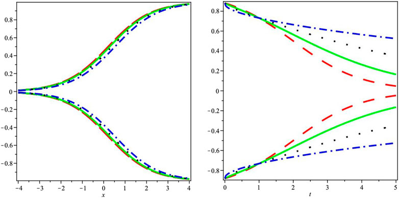
FIGURE 1. The first graph demonstrates the two-dimensional fuzzy lower and upper branch graphs for the analytical series solution, while the second graph illustrates the fractional-order differences between the two different series.

Moving on to Figure 2, similar to Figure 1, the first graph displays the two-dimensional fuzzy lower and upper branch graphs representing the analytical series solution. This visualization offers a comprehensive view of the solution's behavior and properties. The second graph in Figure 2 focuses on the fractional-order differences between the two different series of Example 2. By examining this graph, one can observe and analyze the variations and discrepancies in the fractional-order components, gaining a deeper understanding of their influence on the overall solution.

FIGURE 2

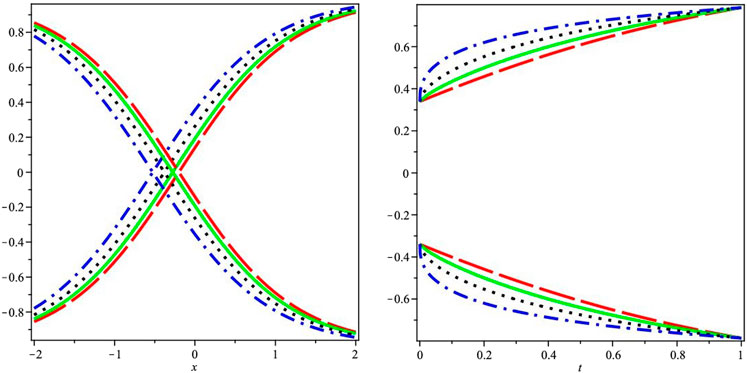
FIGURE 2. The first graph demonstrates the two-dimensional fuzzy lower and upper branch graphs for the analytical series solution, while the second graph illustrates the fractional-order differences between the two different series.

Overall, the graphical discussion presented in Figure 1 and Figure 2 provides a visual representation of the analytical series solutions, allowing for a better comprehension of the fuzzy lower and upper branch graphs as well as the fractional-order differences in the respective examples. These graphical analyses enhance the interpretation and interpretation of the results obtained in the study, contributing to a more comprehensive understanding of the investigated phenomena.

Conclusion

The Atangana–Baleanu operator is used in this work to attempt a semi-analytic solution to the fuzzy fractional Gardner and Cahn–Hilliard equations. As a result, in this case, fuzzy operators are better suited to describe the physical phenomena. Using a fuzzy method that takes into account the starting condition’s uncertainty, we computed the solutions to the Gardner and Cahn–Hilliard equations. This study generalized the fuzzy fractional of the Gardner and Cahn–Hilliard equations. Next, we created the approximate parametric formulation of the suggested problem using a novel iterative transform technique. We demonstrated many examples that supported the methodology’s intended use and created a parametric solution for each case. Last but not least, solving a wide variety of fuzzy fractional partial differential equations analytically is not an easy task.

Data availability statement

The raw data supporting the conclusion of this article will be made available by the authors, without undue reservation.

Author contributions

All authors listed have made a substantial, direct, and intellectual contribution to the work and approved it for publication.

Funding

This work was supported by the Deanship of Scientific Research, the Vice Presidency for Graduate Studies and Scientific Research, King Faisal University, Saudi Arabia (Grant No. 3661).

Conflict of interest

The authors declare that the research was conducted in the absence of any commercial or financial relationships that could be construed as a potential conflict of interest.

Publisher’s note

All claims expressed in this article are solely those of the authors and do not necessarily represent those of their affiliated organizations, or those of the publisher, the editors, and the reviewers. Any product that may be evaluated in this article, or claim that may be made by its manufacturer, is not guaranteed or endorsed by the publisher.

References

1 Baleanu D, Jajarmi A, Mohammadi H, Rezapour S. A new study on the mathematical modelling of human liver with Caputo-Fabrizio fractional derivative. Chaos, Solitons and Fractals (2020) 134:109705. doi:10.1016/j.chaos.2020.109705

CrossRef Full Text | Google Scholar

2 Attia N, Akgul A, Seba D, Nour A, Asad J. A novel method for fractal-fractional differential equations. Alexandria Eng J (2022) 61(12):9733–48. doi:10.1016/j.aej.2022.02.004

CrossRef Full Text | Google Scholar

3 Baleanu D, Ghassabzade FA, Nieto JJ, Jajarmi A. On a new and generalized fractional model for a real cholera outbreak. Alexandria Eng J (2022) 61(11):9175–86. doi:10.1016/j.aej.2022.02.054

CrossRef Full Text | Google Scholar

4 Asjad MI, Usman M, Kaleem MM, Akgul A. Numerical solutions of fractional Oldroyd-B hybrid nanofluid through a porous medium for a vertical surface. Waves in Random and Complex Media (2022) 1–21. doi:10.1080/17455030.2022.2128233

CrossRef Full Text | Google Scholar

5 Datta DP. The golden mean, scale free extension of real number system, fuzzy sets and 1/f spectrum in physics and biology. Chaos, Solitons and Fractals (2003) 17(4):781–8. doi:10.1016/s0960-0779(02)00531-3

CrossRef Full Text | Google Scholar

6 Haq EU, Hassan QMU, Ahmad J, Ehsan K. Fuzzy solution of system of fuzzy fractional problems using a reliable method. Alexandria Eng J (2022) 61(4):3051–8. doi:10.1016/j.aej.2021.08.034

CrossRef Full Text | Google Scholar

7 El Naschie MS. On a fuzzy Kahler-like manifold which is consistent with the two slit experiment. Int J Nonlinear Sci Numer Simulation (2005) 6(2):95–8. doi:10.1515/ijnsns.2005.6.2.95

CrossRef Full Text | Google Scholar

8 El Naschie MS. From experimental quantum optics to quantum gravity via a fuzzy Kahler manifold. Chaos, Solitons and Fractals (2005) 25(5):969–77. doi:10.1016/j.chaos.2005.02.028

CrossRef Full Text | Google Scholar

9 Zadeh LA. Fuzzy sets. In: Fuzzy sets, fuzzy logic, and fuzzy systems: Selected papers by lotfi A zadeh. Singapore: World Scientific Publishing Co. Inc (1996). p. 394–432.

CrossRef Full Text | Google Scholar

10 Chang SS, Zadeh LA. On fuzzy mapping and control. In: Fuzzy sets, fuzzy logic, and fuzzy systems: Selected papers by lotfi A zadeh. Singapore: World Scientific Publishing Co. Inc (1996). p. 180–4.

CrossRef Full Text | Google Scholar

11 Zadeh LA. Linguistic variables, approximate reasoning and dispositions. Med Inform (1983) 8(3):173–86. doi:10.3109/14639238309016081

CrossRef Full Text | Google Scholar

12 Mizumoto M, Tanaka K. The four operations of arithmetic on fuzzy numbers. Syst Comput Controls (1976) 7(5):73–81.

Google Scholar

13 Mizumoto M, Tanaka K. Some properties of fuzzy sets of type 2. Inf Control (1976) 31(4):312–40. doi:10.1016/s0019-9958(76)80011-3

CrossRef Full Text | Google Scholar

14 Dubois DJ. Fuzzy sets and systems: Theory and applications. New York, NY: Academic Press (1980).

Google Scholar

15 Dubois D, Prade H. Operations on fuzzy numbers. Int J Syst Sci (1978) 9(6):613–26. doi:10.1080/00207727808941724

CrossRef Full Text | Google Scholar

16 Ralescu D. A survey of the representation of fuzzy concepts and its applications. In: Advances in fuzzy set theory and applications. Amsterdam: North Holland (1979). p. 77–91.

Google Scholar

17 Nahmias S. Fuzzy variables. Fuzzy sets Syst (1978) 1(2):97–110. doi:10.1016/0165-0114(78)90011-8

CrossRef Full Text | Google Scholar

18 Negoita CV, Ralecu DA. Applications of fuzzy sets to system analysis. New York, NY: John Wiley and Sons (1975).

Google Scholar

19 Caputo M. Linear models of dissipation whose Q is almost frequency independent. Part II. Ann Geophys (1966) 19(4):383–93. doi:10.1111/j.1365-246X.1967.tb02303.x

CrossRef Full Text | Google Scholar

20 Marin M, Marinescu C. Thermoelasticity of initially stressed bodies, asymptotic equipartition of energies. Int J Eng Sci (1998) 36(1):73–86. doi:10.1016/s0020-7225(97)00019-0

CrossRef Full Text | Google Scholar

21 Marin M. A domain of influence theorem for microstretch elastic materials. Nonlinear Anal Real World Appl (2010) 11(5):3446–52. doi:10.1016/j.nonrwa.2009.12.005

CrossRef Full Text | Google Scholar

22 Miller KS, Ross B. An introduction to the fractional calculus and differential equations. New York, NY: John Wiley (1993).

Google Scholar

23 Podlubny I. Fractional differential equations: An introduction to fractional derivatives, fractional differential equations, to methods of their solution and some of their applications. San Diego, CA: Academic Press (1998).

Google Scholar

24 Rawashdeh SM. An efficient approach for time-fractional damped Burger and time-sharma-tasso-Olver equations using the FRDTM. Appl Math Inf Sci (2015) 9(3):1239–46. doi:10.12785/amis/090317

CrossRef Full Text | Google Scholar

25 Rawashdeh MS, Al-Jammal H. Numerical solutions for systems of nonlinear fractional ordinary differential equations using the FNDM. Mediterr J Math (2016) 13(6):4661–77. doi:10.1007/s00009-016-0768-7

CrossRef Full Text | Google Scholar

26 Arikoglu A, Ozkol I. Solution of fractional differential equations by using differential transform method. Chaos, Solitons and Fractals (2007) 34(5):1473–81. doi:10.1016/j.chaos.2006.09.004

CrossRef Full Text | Google Scholar

27 Khan H, Khan A, Al-Qurashi M, Shah R, Baleanu D. Modified modelling for heat like equations within Caputo operator. Energies (2020) 13(8):2002. doi:10.3390/en13082002

CrossRef Full Text | Google Scholar

28 Momani S, Odibat Z. Analytical solution of a time-fractional Navier-Stokes equation by Adomian decomposition method. Appl Math Comput (2006) 177(2):488–94. doi:10.1016/j.amc.2005.11.025

CrossRef Full Text | Google Scholar

29 Khan H, Khan A, Kumam P, Baleanu D, Arif M. A case report of absolute thrombocytopenia with ticagrelor. Adv Difference Equations (2020) 2020(1):1–5. doi:10.1093/ehjcr/ytaa169

CrossRef Full Text | Google Scholar

30 Wu GC. A fractional variational iteration method for solving fractional nonlinear differential equations. Comput Math Appl (2011) 61(8):2186–90. doi:10.1016/j.camwa.2010.09.010

CrossRef Full Text | Google Scholar

31 Qin Y, Khan A, Ali I, Al Qurashi M, Khan H, Shah R, et al. An efficient analytical approach for the solution of certain fractional-order dynamical systems. Energies (2020) 13(11):2725. doi:10.3390/en13112725

CrossRef Full Text | Google Scholar

32 Rawashdeh MS. The fractional natural decomposition method: Theories and applications. Math Methods Appl Sci (2017) 40(7):2362–76. doi:10.1002/mma.4144

CrossRef Full Text | Google Scholar

33 Gardner GHF, Gardner LW, Gregory AR. Formation velocity and density-the diagnostic basics for stratigraphic traps. Geophysics (1974) 39(6):770–80. doi:10.1190/1.1440465

CrossRef Full Text | Google Scholar

34 Fu Z, Liu S, Liu S. New kinds of solutions to Gardner equation. Chaos Solit Fractals (2004) 20(2):301–9. doi:10.1016/s0960-0779(03)00383-7

CrossRef Full Text | Google Scholar

35 Xu GQ, Li ZB, Liu YP. Exact solutions to a large class of nonlinear evolution equations. Chin J Phys (2003) 41(3):232–41.

Google Scholar

36 Kuo CK. New solitary solutions of the Gardner equation and Whitham-Broer-Kaup equations by the modified simplest equation method. Optik (2017) 147:128–35. doi:10.1016/j.ijleo.2017.08.048

CrossRef Full Text | Google Scholar

37 Cahn JW, Hilliard JE. Free energy of a nonuniform system. I. Interfacial free energy. J Chem Phys (1958) 28(2):258–67. doi:10.1063/1.1744102

CrossRef Full Text | Google Scholar

38 Dahmani Z, Benbachir M. Solutions of the Cahn-Hilliard equation with time- and space-fractional derivatives. Int J Nonlinear Sci (2009) 8(1):19–26. doi:10.1007/3-540-32371-6_3

CrossRef Full Text | Google Scholar

39 Hosseini K, Bekir A, Ansari R. New exact solutions of the conformable time-fractional Cahn-Allen and Cahn-Hilliard equations using the modified Kudryashov method. Optik (2017) 132:203–9. doi:10.1016/j.ijleo.2016.12.032

CrossRef Full Text | Google Scholar

40 Rawashdeh MS, Obeidat NA. Applying the reduced differential transform method to solve the telegraph and Cahn-Hilliard equations. Thai J Math (2015) 13(1):153–63.

Google Scholar

41 Arafa A, Elmahdy G. Application of residual power series method to fractional coupled physical equations arising in fluids flow. Int J Differ Equ (2018) 2018:1–10. doi:10.1155/2018/7692849

CrossRef Full Text | Google Scholar

42 Bouhassoun A, Cherif MH. Homotopy perturbation method for solving the fractional Cahn-Hilliard equation. J Interdiscip Math (2015) 18(5):513–24. doi:10.1080/10288457.2013.867627

CrossRef Full Text | Google Scholar

43 Allahviranloo T. Fuzzy fractional differential operators and equation studies in fuzziness and soft computing. Berlin, Germany: Springer (2021).

Google Scholar

44 Gottwald S. Fuzzy set theory and its applications. Dordrecht: Kluwer Academic Publishers (1992).

Google Scholar

45 Allahviranloo T, Ahmadi MB. Fuzzy laplace transforms. Soft Comput (2010) 14(3):235–43. doi:10.1007/s00500-008-0397-6

CrossRef Full Text | Google Scholar

46 Maitama S, Zhao W. Homotopy analysis Shehu transform method for solving fuzzy differential equations of fractional and integer order derivatives. Comput Appl Math (2021) 40(3):86–30. doi:10.1007/s40314-021-01476-9

CrossRef Full Text | Google Scholar