
94% of researchers rate our articles as excellent or good
Learn more about the work of our research integrity team to safeguard the quality of each article we publish.
Find out more
ORIGINAL RESEARCH article
Front. Phys., 17 April 2023
Sec. Interdisciplinary Physics
Volume 11 - 2023 | https://doi.org/10.3389/fphy.2023.1167797
This article is part of the Research TopicAnalytical Methods for Nonlinear Oscillators and Solitary WavesView all 14 articles
This article circumvents the Laplace transform to provide an analytical solution in a power series form for singular, non-singular, linear, and non-linear ordinary differential equations. It introduces a new analytical approach, the Laplace residual power series, which provides a powerful tool for obtaining accurate analytical and numerical solutions to these equations. It demonstrates the new approach’s effectiveness, accuracy, and applicability in several ordinary differential equations problem. The proposed technique shows the possibility of finding exact solutions when a pattern to the series solution obtained exists; otherwise, only rough estimates can be given. To ensure the accuracy of the generated results, we use three types of errors: actual, relative, and residual error. We compare our results with exact solutions to the problems discussed. We conclude that the current method is simple, easy, and effective in solving non-linear differential equations, considering that the obtained approximate series solutions are in closed form for the actual results. Finally, we would like to point out that both symbolic and numerical quantities are calculated using Mathematica software.
A differential equation or a system of differential equations, along with proper boundary and initial conditions (ICs), is one of the most common outputs when mathematical modeling describes physical, biological, or chemical phenomena. Finding ordinary or partial differential equations and analyzing their solutions are at the heart of applied mathematics [1].
Since ancient times, differential equations have attracted the interest of researchers and scientists from two sides. The first is how to use them to express phenomena and issues that interest them in their specializations and research. On the other hand, there is the question of how to solve these equations. There are a limited number of differential equations, especially linear ones, whose solutions can be determined using the well-known traditional methods based on finite and simple algebraic operations. In contrast, there are many kinds of differential equations that still require the search for simple and accurate solutions. For this reason, the interest of mathematicians in previous decades was and is still in the investigation for analytical and sometimes numerical methods to solve these forms of differential equations.
Many analytical, numerical, and numero-analytical techniques have been proposed previously and recently to provide solutions for differential equations with initial or boundary conditions, such as the Laplace and Fourier transforms method [2], the Adomian decomposition method [3–5], the variational iteration method [6–8], the homotopy perturbation method [9–11], the homotopy analysis method [12, 13], the differential transformation method [14–16], the finite difference method [17], the predictor–corrector method [18, 19], the first integral method [20, 21], the Adams–Bashforth Molten method [22], the new iterative method [23, 24], the Crank–Nicolson method [25, 26], the reproducing kernel method [27, 28], the Laplace Adomian decomposition method [11, 29, 30], the He–Laplace method [31–33], and others [34–36].
Recently, Eriqat et al. [37] presented a new hybrid method in which they combined the Laplace transform (LT) method with the residual power series (PS) method to establish series solutions of the pantograph equation. This method is called the LRPS method, and it simulates the residual PS method but with a different construction and view. It uses the limit concept instead of the concept of the derivative as in the residual PS method. The LRPS method uses the LT to transfer the given differential equation to a new algebraic equation in a new space. The obtained algebraic equation is solved by assuming that it is a solution that has a Laurent series (LS) form. The values of the coefficients of the LS are determined by utilizing the limit at infinity. Then, the inverse LT is used to transfer the LS, which is the solution of the algebraic equation in the Laplace space, to the initial space. Thus, we have obtained the solution to the original problem in the form of PS.
Indeed, the LRPS method is similar to the He–Laplace method’s [31–33] idea of searching for the solution of differential equations in Laplace space. The He–Laplace technique uses the variational iteration method or homotopy perturbation method to solve the just-transformed Laplace space. In contrast, the LRPS method uses the PS method to solve that equation using the Laurent series instead of the Taylor series. In addition, the LRPS method is just an easy and fast technique for finding the PS solution coefficients of the differential equations.
The LRPS method has won the admiration and interest of many researchers due to its ease, speed, and efficiency in arriving at exact or accurate approximate solutions to many equations. In addition, the LT was employed in dealing with non-linear problems because it is known that the LT deals only with some categories of linear equations. In 2021, El-Ajou [38] adapted the LRPS method to establish solitary solutions of non-linear time-fractional dispersive partial differential equations and to introduce a vector series solution of some types of hyperbolic system of Caputo time-fractional partial differential equations with variable coefficients [39]. Recently, the LRPS method was used for solving time-fractional Navier–Stokes equations [40], fuzzy quadratic Riccati DEs [41], Lane–Emden equations of fractional order [42], a system of fractional initial value problems (IVPs) [43], autonomous n-dimensional fractional non-linear systems [44], and others [45–49].
Despite the extensive publication of research dealing with the new method, all works dealt with specific problems devoid of complexity and generality. Therefore, we aim in this manuscript, first, to employ the LRPS method to provide exact or accurate approximate analytic series solutions to linear ordinary differential equations (ODEs) in their general form, whether their coefficients are constants or analytical functions, which have the following formula:
Subject to the ICs,
where
Since in our world, most events are essentially non-linear and modeled by non-linear equations, the study of non-linear issues is critical in mathematics and physics, engineering, economics, and other disciplines. Solving non-linear problems is difficult, and getting an analytical approximation of a given problem is often more complicated than getting a numerical one. Therefore, the second aim of this paper is to establish analytic approximate solutions to the general form of non-linear ODEs, which have the following form using the proposed method (LRPS method):
Subject to the ICs,
where
The third objective of this article is to provide a series solution to the singular ODEs, whether linear or non-linear. This type of equation is of great interest to researchers in providing analytical solutions to it, as it appears in the models of many natural phenomena, as well as the difficulty of providing solutions to it.
To determine the efficiency and applicability of the method, we test for three types of errors: exact error, relative error, and residual error. We present the numerical results of the resulting solutions through prepared and organized tables. In addition, we sketch the obtained approximate solution by the proposed method along with the exact solution if we can obtain it to make the comparison on the one hand and to determine the period of convergence to solve the series on the other hand.
In this section, we overview essential facts about the LT and the PS, along with some properties that are needed in this article.
Definition 2.1. [50]). We assume that
where the improper integral is the convergence on an interval of
where
Lemma 2.1. [50]). Suppose that
1)
2)
3)
4)
6)
Definition 2.2. [51]). A series that has the representation
is called the LS about
Theorem 2.1. [50]). Let
which is valid for
Theorem 2.2. If
then
According to part (5) of Lemma 2.1, we have
Using part (5) of Lemma 2.1, it is obvious that
Similarly, multiplying Eq. 2.7 by
Again, by parts (5) and (6) of Lemma 2.1, we have
Now, we can find out the general formula for the coefficient
Theorem 2.3. assume that
Proof.First, we assume that for
From the definition of the reminder
Eq. 2.10 and Eq. 2.11 lead to the conclusion that
The inequality
In this section, we first use the LRPS method to solve linear ODEs in preparation for solving non-linear ODEs. What is worth noting is the possibility of solving non-linear ODEs, which cannot be carried out using the traditional LT method. We will use the construction that we will get to solve non-linear ODEs when solving singular ODEs, whether linear or non-linear, and this is what we will see in Section 3.3.
In this section, we demonstrate the steps of the LRPS method for solving linear ODEs. The basic idea of the proposed method is to apply the LT to the linear ODEs and then use the LRPS approach to construct a series solution, in LS form, to the transformed equation. Then, we transform the obtained solution into the required solution in the original space.
To illustrate the idea of the LRPS method in constructing series solutions to the linear ODEs, we consider problems (1.1) and (1.2), considering that
where
To generate the LRPS solution of the IVP (1.1) and (1.2), first, we apply the LT to both sides of Eq. 1.1 to obtain
Using ICs (1.2) and some properties of the LT, Eq. 3.2 becomes
We assume that
Depending on Theorem 2.3 and the given conditions in Eq. 1.2, the first
The
Thus, one can conclude
To find the values of the unknown coefficients in series (3.7), we define the Laplace residual function (LRF) of Eq. 3.3 as
and the
It is clear that
Substituting the first
Running the inverse LT in Eq. 3.11, we get
Since the coefficients of the linear operator in Eq. 3.1 are analytic functions, they can be expressed as
where
So, the linear operator
Running the operator
Finally, we run the LT in Eq. 3.16 to obtain the required form of the
Now, multiplying Eq. 3.17 by
Taking the limit at infinity to Eq. 3.18, according to Eq. 3.10, we get
Thus, the first approximation of the solution of Eq. 3.3 is
Following that, one can find the value of the coefficient
Performing the previous steps, we obtain the final form of the
Again, we multiply Eq. 3.22 by
Computing the limit at infinity to both sides of the last equation and using Eq. 3.10, we get
So, the second approximation of the solution of Eq. 3.3 is
Like the previous steps, we have
Repeating the steps, one can obtain
Considering a pattern of the obtained coefficients, we easily deduce the coefficient
According to Eq. 3.14, the recurrence relation (3.28) becomes as follows:
Thus, we can express the
Therefore, the exact solution of Eq. 3.3 can be expressed as
Substituting the result in Eq. 3.29 into Eq. 3.31 and running the inverse LT gives the solutions of IVP (1.1) and (1.2) as follows:
This section introduces the steps of the LRPS approach in solving non-linear ODEs. To explain the methodology of the proposed method in constructing series solutions to this class, we consider IVP (1.3) and (1.4).
To generate the LRPS solution of the IVP (1.3) and (1.4), we consider the first step; that is, operating the LT to Eq. 1.3 and utilizing conditions (1.4), we obtain
where
We assume that
To set the values of the unknown coefficients in Eq. 3.6, according to Eq. 3.33, we define the LRF of Eq. 3.33 as
and the kth LRF as
According to the form of
where
Substituting the expansions (3.6) and (3.36) in (3.35) gives the following expansion form of the
Thus, the
Now, we multiply Eq. 3.38 by
Now, applying the limit as s → ∞ to both sides of Eq. 3.39 and using the fact in Eq. 3.10, we can easily determine the value of
In the same manner, we find the value of the coefficient
Multiplying
Applying the limit at infinity to Eq. 3.42, we obtain the algebraic equation:
Solving Eq. 3.43 implicitly for
Similarly, we compute the third coefficient
Multiplying Eq. 3.44 by
According to fact (3.10), we obtain
Solving Eq. 3.46 for
The value of the third unknown coefficient
Considering the pattern of the obtained coefficients, we easily conclude the coefficient
Thus, we can express the
Therefore, the exact analytic solution of Eq. 3.33 is written in a series form:
Running the inverse LT to Eq. 3.50 gives the solution of Eq. 1.3 and Eq. 1.4 in a series expansion as
This section presents the LRPS method’s procedure for handling singular-value problems. To do this, let us consider the following singular-value problem:
Subject to the ICs
To solve the initial-singular value problems (3.52) and (3.53), we first multiply Eq. 3.52 by
Now applying LT to Eq. 3.54 and using ICs (3.53), we get
Now, suppose that the function Y(s) can be expressed in the form of the expansion of (3.4), and so on. We can complete the steps described in the previous Section 3.2 to obtain the required solution.
This section presents seven interesting problems with wide applications in physics and other sciences that are discussed and solved by the LRPS method.
Problem 4.1. consider the following composite oscillation equation:
with respect to the initial condition
Comparing Eq. 4.1 with Eq. 1.1 concludes that
It is easy to check if the exact solution of Eq. 4.1 and Eq. 4.2 is as follows:
To analyze the accuracy of the approximate solution in Eq. 4.3 and determine the interval of convergence, we introduce and compute two types of error, actual and relative errors that are defined, respectively, as follows:
and
For analysis and comparison of the exact and approximate solutions of IVP (4.1) and (4.2), Table 1 shows the numerical results of this problem. It displays the exact and approximate results in addition to the actual and relative errors at different values of
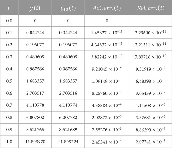
TABLE 1. The exact and the
Problem 4.2. consider the following Bessel’s equation:
Subject to the ICs,
According to the existence and uniqueness theorem, it is clear that the IVPs (4.7) and (4.8) have a unique solution in the interval
Comparing Eq. 4.7 with Eq. 1.1, we find that
where
So, according to Eq. 4.11 and Eq. 3.14, we have
Comparing with the general formula (3.29), we can find the values of the coefficients as follows:
Therefore, the LRPS solution to Problem 4.2 can be expressed in the following series form:
The expansion in (4.13) is the same expansion as that of the function
Table 2 shows the numerical results of Problem 4.2. It shows the exact and approximate results in addition to the actual and relative errors at different values of
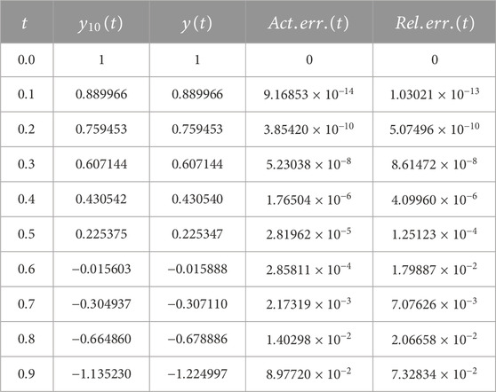
TABLE 2. The exact and the
Problem 4.3. consider the following non-linear nonhomogeneous ODE:
Subject to the ICs,
Similar to the previous problems, we operate the LT on both sides of Eq. 4.15 and employ the ICs (4.16). Then, we obtain the following equation in the Laplace space:
We assume that the solution of Eq. 4.17 has the same LS expansion as in Eq. 3.4. According to ICs (4.16), the
To set the value of the unknown coefficients in series (4.18), we utilize the kth LRF of Eq. 3.17, which is defined as
To determine the coefficient
Employing fact (3.10), the solution of the equation
Utilizing fact (3.10) via Eq. 4.21 gives
Therefore, the LRPS solution to Eq. 4.15 and Eq. 4.16 can be expressed in the following series form:
which is the expansion of the exact solution
Problem 4.4. consider the following non-linear pantograph equation:
Subject to the ICs,
Following the same procedure as in the previous problems, we can express the LRPS solution to IVP (4.24) and (4.25) in the form
Since we cannot predict the pattern in the coefficients of the series solution in Eq. 4.26, we cannot reach the exact solution. Therefore, we test the results using the residual and relative errors, which are defined as follows, respectively:
Table 3 shows the numerical results of Problem 4.4. It displays the 10th approximate solution in addition to the residual and relative errors at different values of
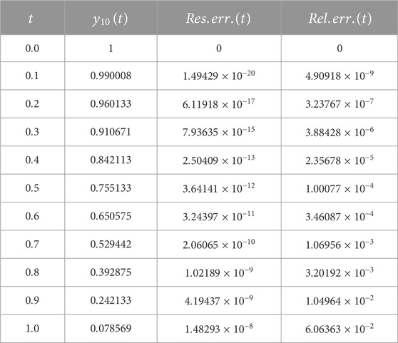
TABLE 3. The
Problem 4.5. consider the following homogenous linear singular ODE:
with respect to the ICs:
We apply the LT on both sides of Eq. 4.29 and use the ICs in Eq. 4.30 to obtain the following symbolic algebraic equation in the Laplace space:
Suppose that the solution of Eq. 4.31 has a LS expansion as in Eq. 3.4. According to ICs (4.30), the
To set the unknown coefficient in series (4.32), we define the
We substitute
Solving the equation
Consequently, the equation
Solving the equation
Applying the inverse LT to Eq. 4.38 gives the LRPS solution to the IVP (4.29) and (4.30) in the following PS form:
It is clear that the closed form of the exact solution of IVP (4.50) and (4.51) is
Problem 4.6. consider the following non-homogeneous nonlinear Lane–Emden singular ODE:
considering the ICs:
Using similar arguments to the previous problem, one can obtain the series solution of the LT of the IVP (4.40) and (4.41) as follows:
Applying the inverse LT on Eq. 4.42 gives the LRPS solution of the IVP (4.40) (4.41) in the following series form:
There is no pattern between the series terms in Eq. 4.43. So, it is difficult to predict the exact solution formula. Thus, we suffice with the approximate solution we got for Problem 4.6. It is worth noting that the more terms we calculate for the LRPS solution, the longer the series convergence interval and the higher the accuracy of the solution. Therefore, we test the 8th approximate LRPS solution for Problem 4.6 using the residual and relative errors, which are defined as follows, respectively:
Table 4 shows the numerical results of Problem 4.6. It illustrates the 8th approximate solution in addition to the residual and relative errors at different values of
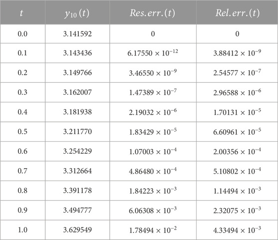
TABLE 4. The
Problem 4.7. We consider the following micro-electromechanical system (MEMS) [52]:
with the ICs:
This dynamic differential equation is used to describe the wire’s movement as a point mass, where
Simulating the previous examples, the LT of the IVP (4.46) and (4.47) is given by the following algebraic equation:
Applying the arguments and processes of the LRPS method, one can obtain the LRPS solution to the algebraic Eq. 4.48 as follows:
Applying the inverse LT to Eq. 4.49 gives the LRPS solution of the IVP (4.46) (4.47) as follows:
To test the accuracy of the obtained solution given in (4.50), we compute the residual and relative errors to the 10th approximation of the solution. Table 5 shows the 10th approximate solution in addition to the residual and relative errors at different values of
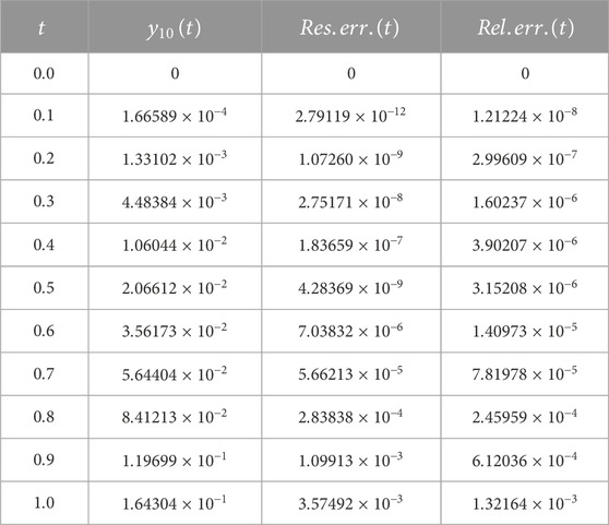
TABLE 5. The
On the other hand, what specialists in MEMS system implementations are most interested in is the pull-in phenomenon analysis. The MEMS system in Eq. 4.46 and Eq. 4.47 conducts either periodically or unsteadily. This behavior depends on the value of the voltage-related parameter,
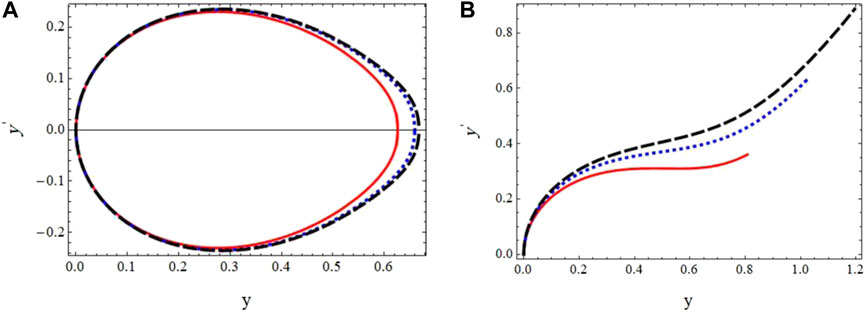
FIGURE 1. Phase trajectories at different values of
This study aims to test the efficiency of the LRPS method in finding series solutions for ODEs, which are difficult to solve in the analytical methods. We have succeeded in providing a solution to the general form of linear ODEs whose coefficients are analytical functions as an exact solution in a PS form. We also dealt with non-linear ODEs in the proposed technique and found approximate solutions with high accuracy. The biggest surprise is the success of the LRPS method in providing series solutions for the equations about the singular points that coincide with the exact results in some examples. Using the LRPS method, there is no longer an obstacle to obtaining a PS solution for a broad class of ODEs. In addition, the idea of the method circumvented the use of the LT to solve non-linear equations to which the LT is difficult to apply. In addition to the method’s efficiency in arriving at exact solutions, LRPS is easy and fast in finding the coefficients of a series solution. There is no doubt that we can use the new method to solve other sets of equations that we did not have to deal with in previous studies, such as using it to solve partial differential equations, integral equations, integrodifferential equations, and linear or non-linear, as well as algebraic equations. We should not forget that the method has not been applied to solve differential equations with boundary conditions. All these and other topics will be under research by our research team in the next stage.
The original contributions presented in the study are included in the article/Supplementary Material; further inquiries can be directed to the corresponding author.
All authors listed have made a substantial, direct, and intellectual contribution to the work and approved it for publication.
The authors declare that the research was conducted in the absence of any commercial or financial relationships that could be construed as a potential conflict of interest.
All claims expressed in this article are solely those of the authors and do not necessarily represent those of their affiliated organizations, or those of the publisher, the editors, and the reviewers. Any product that may be evaluated in this article, or claim that may be made by its manufacturer, is not guaranteed or endorsed by the publisher.
1. King A, Billingham J, Otto S. Differential equations: Linear, nonlinear, ordinary and partial. Cambridge: Cambridge University Press (2003).
2. Huntley E, Pickering WM, Zinober ASI. The numerical solution of linear time-dependent partial differential equations by the Laplace and fast Fourier transforms. J Comput Phys (1978) 27(2):256–71. doi:10.1016/0021-9991(78)90008-6
3. Adomian G. A review of the decomposition method and some recent results for nonlinear equations. Comput Maths Appl (1991) 21(5):101–27. doi:10.1016/0898-1221(91)90220-x
4. Evans DJ, Raslan KR. The Adomian decomposition method for solving delay differential equation. Int J Comput Maths (2005) 82(1):49–54. doi:10.1080/00207160412331286815
5. Ibijola EA, Adegboyegun BJ, Halid OY. On Adomian Decomposition Method (ADM) for numerical solution of ordinary differential equations. Adv Nat Appl Sci (2008) 2(3):165–70.
6. He JH. Approximate solution of nonlinear differential equations with convolution product nonlinearities. Comput Methods Appl Mech Eng (1998) 167(1-2):69–73. doi:10.1016/s0045-7825(98)00109-1
7. He JH. Variational iteration method–a kind of non-linear analytical technique: Some examples. Int J non-linear Mech (1999) 34(4):699–708. doi:10.1016/s0020-7462(98)00048-1
8. Abbasbandy S. Numerical solution of non-linear Klein–Gordon equations by variational iteration method. Int J Numer Methods Eng (2007) 70(7):876–81. doi:10.1002/nme.1924
9. Anjum N, He JH, Ain QT, Tian D. Li-He’s modified homotopy perturbation method for doubly-clamped electrically actuated microbeams-based microelectromechanical system. Facta Universitatis, Ser Mech Eng (2021) 19(4):601–12. . doi:10.22190/fume210112025a
10. Anjum N, He JH. Homotopy perturbation method for N/MEMS oscillators. In: Mathematical methods in the applied sciences (2020). .
11. Saadeh R. Numerical algorithm to solve a coupled system of fractional order using a novel reproducing kernel method. Alexandria Eng J (2021) 60(5):4583–91. doi:10.1016/j.aej.2021.03.033
12. Liao W, Zhu J, Khaliq AQ. An efficient high-order algorithm for solving systems of reaction-diffusion equations. Numer Methods Partial Differential Equations (2002) 18(3):340–54. doi:10.1002/num.10012
13. Abbasbandy S. Soliton solutions for the Fitzhugh–Nagumo equation with the homotopy analysis method. Appl Math Model (2008) 32(12):2706–14. doi:10.1016/j.apm.2007.09.019
14. Pukhov G. Taylor transforms and their application in electrical engineering and electronics (Russian book). Kiev: Izdatel'stvo Naukova Dumka (1978). p. 259. p, In Russian.
15. Pukhov GE. Differential transformations of functions and equations. Kiev: Naukova Dumka (1980). p. 54–7. (in Russian).
16. Abbasov TEYMURAZ, Bahadir AR. The investigation of the transient regimes in the nonlinear systems by the generalized classical method. Math Probl Eng (2005) 2005(5):503–19. doi:10.1155/mpe.2005.503
17. Chawla M. A fourth-order tridiagonal finite difference method for general non-linear two-point boundary value problems with mixed boundary conditions. IMA J Appl Maths (1978) 21(1):83–93. doi:10.1093/imamat/21.1.83
18. Ascher UM, Ruuth SJ, Wetton BT. Implicit-explicit methods for time-dependent partial differential equations. SIAM J Numer Anal (1995) 32(3):797–823. doi:10.1137/0732037
19. Burrage K, Tian T. Predictor-corrector methods of runge--kutta type for stochastic differential equations. SIAM J Numer Anal (2002) 40(4):1516–37. doi:10.1137/s0036142900372677
20. Feng Z, Knobel R. Traveling waves to a Burgers–Korteweg–de Vries-type equation with higher-order nonlinearities. J Math Anal Appl (2007) 328(2):1435–50. doi:10.1016/j.jmaa.2006.05.085
21. Eslami M, Fathi Vajargah B, Mirzazadeh M, Biswas A. Application of first integral method to fractional partial differential equations. Indian J Phys (2014) 88(2):177–84. doi:10.1007/s12648-013-0401-6
22. Ascher UM, Petzold LR. Computer methods for ordinary differential equations and differential-algebraic equations. Philadelphia, PA: Society for Industrial and Applied Mathematics (1998). p. 61.
23. Ostrowski AM. Solution of equations and systems of equations: Pure and applied mathematics: A series of monographs and textbooks, vol. 9. Amsterdam: Elsevier (2016).
24. Hueso JL, Martínez E, Teruel C. Multipoint efficient iterative methods and the dynamics of Ostrowski's method. Int J Comput Maths (2019) 96(9):1687–701. doi:10.1080/00207160.2015.1080354
25. Li D, Zhang C. Nonlinear stability of discontinuous Galerkin methods for delay differential equations. Appl Maths Lett (2010) 23(4):457–61. doi:10.1016/j.aml.2009.12.003
26. Zaibin Z, Zhizhong S. A Crank-Nicolson scheme for a class of delay nonlinear parabolic differential equations. J Numerica Methods Comput Appl (2010) 31(2):131.
27. Zhou Y, Cui M, Lin Y. Numerical algorithm for parabolic problems with non-classical conditions. J Comput Appl Maths (2009) 230(2):770–80. doi:10.1016/j.cam.2009.01.012
28. Geng F, Cui M. A reproducing kernel method for solving nonlocal fractional boundary value problems. Appl Maths Lett (2012) 25(5):818–23. doi:10.1016/j.aml.2011.10.025
29. Khuri SA. A Laplace decomposition algorithm applied to a class of nonlinear differential equations. J Appl Math (2001) 1(4):141–55. doi:10.1155/s1110757x01000183
30. Kiymaz O. An algorithm for solving initial value problems using Laplace Adomian decomposition method. Appl Math Sci (2009) 3:1453–9.
31. Nadeem M, He JH. He–Laplace variational iteration method for solving the nonlinear equations arising in chemical kinetics and population dynamics. J Math Chem (2021) 59:1234–45. doi:10.1007/s10910-021-01236-4
32. Rehman S, Hussain A, Rahman JU, Anjum N, Munir T. Modified Laplace based variational iteration method for the mechanical vibrations and its applications. acta mechanica et automatica (2022) 16(2):98–102. . doi:10.2478/ama-2022-0012
33. Anjum N, He JH. Laplace transform: Making the variational iteration method easier. Appl Maths Lett (2019) 92:134–8. . doi:10.1016/j.aml.2019.01.016
34. He K, Nadeem M, Habib S, Sedighi HM, Huang D. Analytical approach for the temperature distribution in the casting-mould heterogeneous system. Int J Numer Methods Heat Fluid flow (2022) 32(3):1168–82. . doi:10.1108/hff-03-2021-0180
35. Fang J, Nadeem M, Habib M, Karim S, Wahash HA. A new iterative method for the approximate solution of klein-gordon and sine-gordon equations. J Funct Spaces (2022) 2022:1–9. doi:10.1155/2022/5365810
36. Anjum N, Suleman M, Lu D, He JH, Ramzan M. Numerical iteration for nonlinear oscillators by Elzaki transform. J Low Frequency Noise, Vibration Active Control (2020) 39(4):879–84. . doi:10.1177/1461348419873470
37. Eriqat T, El-Ajou A, Oqielat MN, Al-Zhour Z, Momani S. A new attractive analytic approach for solutions of linear and nonlinear neutral fractional pantograph equations. Chaos, Solitons and Fractals (2020) 138:109957. doi:10.1016/j.chaos.2020.109957
38. El-Ajou A. Adapting the Laplace transform to create solitary solutions for the nonlinear time-fractional dispersive PDEs via a new approach. The Eur Phys J Plus (2021) 136(2):229–2. doi:10.1140/epjp/s13360-020-01061-9
39. El-Ajou A, Al-Zhour Z. A vector series solution for a class of hyperbolic system of Caputo time-fractional partial differential equations with variable coefficients. Front Phys (2021) 9:525250. doi:10.3389/fphy.2021.525250
40. Burqan A, El-Ajou A, Saadeh R, Al-Smadi M. A new efficient technique using Laplace transforms and smooth expansions to construct a series solution to the time-fractional Navier-Stokes equations. Alexandria Eng J (2022) 61(2):1069–77. doi:10.1016/j.aej.2021.07.020
41. Oqielat MN, El-Ajou A, Al-Zhour Z, Eriqat T, Al-Smadi M. A new approach to solving fuzzy quadratic Riccati differential equations. Int J Fuzzy Logic Intell Syst (2022) 22(1):23–47. . doi:10.5391/ijfis.2022.22.1.23
42. Saadeh R, Burqan A, El-Ajou A. Reliable solutions to fractional Lane-Emden equations via Laplace transform and residual error function. Alexandria Eng J (2022) 61(12):10551–62. doi:10.1016/j.aej.2022.04.004
43. Salah E, Qazza A, Saadeh R, El-Ajou A. A hybrid analytical technique for solving multi-dimensional time-fractional Navier-Stokes system. AIMS Maths (2023) 8(1):1713–36. doi:10.3934/math.2023088
44. Alquran M, Ali M, Alshboul O. Explicit solutions to the time-fractional generalized dissipative Kawahara equation. J Ocean Eng Sci (2022) 1–5. doi:10.1016/j.joes.2022.02.013
45. Eriqat T, Oqielat MN, Al-Zhour Z, Khammash G, El-Ajou A, Alrabaiah H. Exact and numerical solutions of higher-order fractional partial differential equations: A new analytical method and some applications. Pramana (2022) 96(4):207. doi:10.1007/s12043-022-02446-4
46. Saadeh R, Ala’yed O, Qazza A. Analytical solution of coupled hirota–satsuma and KdV equations. Fractal and Fractional (2022) 6(12), 694. doi:10.3390/fractalfract6120694
47. Saadeh R, Qazza A, Amawi K. A new approach using integral transform to solve cancer models. Fractal and Fractional (2022) 6(9), 490.doi:10.3390/fractalfract6090490
48. El-Ajou A, Oqielat MN, Al-Zhour Z, Momani S. A class of linear non-homogenous higher order matrix fractional differential equations: Analytical solutions and new technique. Fractional Calculus Appl Anal (2020) 23(2), 356–77. doi:10.1515/fca-2020-0017
49. Eriqat T, Oqielat MN, Al-Zhour Z, El-Ajou A, Bataineh A. Revisited Fisher’s equation and logistic system model: A new fractional approach and some modifications. Int J Dyn Control (2022) 11, 555–63. doi:10.1007/s40435-022-01020-5
50. Nagle RK, Saff EB, Snider AD. Fundamentals of differential equations. United States: Pearson (2018).
51. Zill DG, Shanahan PD. A first course in complex analysis with applications. London: Jones & Bartlett Learning (2013).
Keywords: ordinary differential equations, Laplace transforms, power series, approximate solutions, laurent series
Citation: El-Ajou A, Al-ghananeem H, Saadeh R, Qazza A and Oqielat MN (2023) A modern analytic method to solve singular and non-singular linear and non-linear differential equations. Front. Phys. 11:1167797. doi: 10.3389/fphy.2023.1167797
Received: 16 February 2023; Accepted: 23 March 2023;
Published: 17 April 2023.
Edited by:
Ji-Huan He, Soochow University, ChinaReviewed by:
Muhammad Nadeem, Qujing Normal University, ChinaCopyright © 2023 El-Ajou, Al-ghananeem, Saadeh, Qazza and Oqielat. This is an open-access article distributed under the terms of the Creative Commons Attribution License (CC BY). The use, distribution or reproduction in other forums is permitted, provided the original author(s) and the copyright owner(s) are credited and that the original publication in this journal is cited, in accordance with accepted academic practice. No use, distribution or reproduction is permitted which does not comply with these terms.
*Correspondence: Rania Saadeh, cnNhYWRlaEB6dS5lZHUuam8=, cmFuaWFyYWVkMjAxMUBnbWFpbC5jb20=
Disclaimer: All claims expressed in this article are solely those of the authors and do not necessarily represent those of their affiliated organizations, or those of the publisher, the editors and the reviewers. Any product that may be evaluated in this article or claim that may be made by its manufacturer is not guaranteed or endorsed by the publisher.
Research integrity at Frontiers

Learn more about the work of our research integrity team to safeguard the quality of each article we publish.