Fault-tolerant quaternary belief propagation decoding based on a neural network

The article discusses the challenge of finding an efficient decoder for quantum error correction codes for fault-tolerant experiments in quantum computing. The study aims to develop a better decoding scheme based on the flag-bridge fault tolerance experiment. The research compares two decoding algorithms, a deep neural network decoding scheme and a simple decoder, and a recurrent neural network decoding scheme based on the belief propagation algorithm variant MBP₄ algorithm. The study improved the syndrome extraction circuit based on the flag-bridge method to meet the requirements of fault-tolerant experiments better. Two decoding schemes were studied, a combination of a deep neural network and a simple decoder and a recurrent neural network structure based on the MBP₄ algorithm. The first scheme used neural networks to assist simple decoders in determining whether additional logical corrections need to be added. The second scheme used a recurrent neural network structure designed through the variant MBP₄ algorithm, along with a post-processing method to pinpoint the error qubit position for decoding. Experimental results showed that the decoding scheme developed in the study improved the pseudo-threshold by 39.52% compared to the minimum-weight perfect matching decoder. The two decoders had thresholds of approximately 15.8% and 16.4%, respectively. The study’s findings suggest that the proposed decoding schemes could improve quantum error correction and fault-tolerant experiments in quantum computing.

1 Introduction

For reliable implementation of quantum algorithms, fault-tolerant (FT) [1,2] quantum error correction techniques are essential. Fault tolerance can be implemented by quantum error correction (QEC) [3,4], where a single logical qubit is encoded into the state of multiple physical qubits by a QEC code to enable active diagnosis and correction of potential errors. This process should all be FT. As an example of topological QEC codes [5,6], surface codes have emerged as a prime candidate for large-scale FT quantum computing. However, finding the optimal decoding strategy is already a computationally difficult problem. Various decoding algorithms have been proposed such as the Blossom algorithm [7], the maximum likelihood algorithm decoding (MLD) [8], the renormalization group algorithm (RG) [9], and the minimum-weight perfect matching (MWPM) [10]. Recently, machine learning has started to be applied, and to solve the fast decoding problem, the development of neural network-based decoding algorithms [11–17] has increased. Such algorithms require less time, and decoding can achieve a performance similar to that of classical decoding algorithms. Particularly, machine learning-based approaches have a variety of decoding algorithms with great promise, some of which have addressed completely FT environments and satisfied FT trials [18,19]. Meanwhile, the development of deep learning [20,21] algorithms has also made good progress, allowing more room for the development of neural network-based decoding algorithms. On the other hand, sparse error correction codes can achieve good decoding performance through belief propagation (BP) [22,23] because the BP algorithm can achieve nearly linear complexity. Even so, BP is less effective on highly degenerate error correction codes. Due to the existence of short cycles in the Tanner graph of the stabilizer code, this affects the message passing process in BP and may result in additional computational burden.

FT quantum error correction schemes applied to various stabilizer codes are essential but require many ancilla qubits, which are a scarce resource in quantum processors. To solve this problem, the flag QEC scheme is proposed, where only one or a few additional ancilla qubits are added for low overhead and FT implementation of the syndrome extraction circuit. These additional qubits are called flag qubits [24,25]. However, the flag scheme has stringent requirements for qubit connectivity. To achieve this high qubit connectivity, additional operations (e.g., SWAP gates) are usually required, increasing the circuit’s size. More importantly, the resulting circuits, after applying these extra operations, may break the fault tolerance. Based on this, the flag-bridge approach [26] is proposed to extend the flag circuit into various equivalent circuits for FT execution of stabilizer measurements. A pressing problem in this flag-bridge scheme is the design of its decoding algorithm. The flag-bridge scheme requires high-speed decoding algorithms that must be faster than the rate of errors that occur. Therefore, efficiently designing the applicable decoding algorithm is the key to implementing FT quantum computers.

In this work, based on machine learning technology, we propose two decoding strategies in the flag-bridge method: the use of a deep neural decoder (DND) and a recurrent neural network (RNN) decoder based on MBP₄. In the DND strategy, a simple decoder was designed to replace the original non-scalable look-up table strategy, and a depth neural decoder was used to determine whether to add logic correction to the correction of the simple decoder. The simulation results showed that it has a slight improvement compared with the MWPM decoder. In addition, in the second scheme, using the degeneracy of the surface code, through the variant algorithm of the BP algorithm, the RNN decoder was designed and the post-processing method was used to improve the decoding accuracy. The experimental results showed that the numerical value of the latter scheme was higher than that of the former scheme.

The structure of the article is divided into the following parts. In Section 2, the background is described, including topology surface code, flag-bridge fault tolerance, and MBP₄. In Section 3 and Section 4, we introduce the decoder design of the two schemes, respectively. In Section 5, the numerical results and analysis are given. In Section 6, the research content of this article is summarized and the future research direction is indicated.

2 Background

2.1 Surface codes

A code space for a stabilizer code is the joint (+1) eigenspace [27,28] of the elements. The eigenvalues of the stabilizers can be used to determine if a Pauli error anticommutes with some stabilizers. Therefore, a corrective procedure is chosen based on the measurement results, also known as the error syndrome.

The check matrix of the stabilizer code is of the form

$S=\left[S_{mn}\right]\in {\left\{I,X,Y,Z\right\}}^{M\times N},(1)$

where $I=\left[\begin{array}{cc}\hfill 1\hfill & \hfill 0\hfill \\ \hfill 0\hfill & \hfill 1\hfill \end{array}\right],X=\left[\begin{array}{cc}\hfill 0\hfill & \hfill 1\hfill \\ \hfill 1\hfill & \hfill 0\hfill \end{array}\right],Z=\left[\begin{array}{cc}\hfill 1\hfill & \hfill 0\hfill \\ \hfill 0\hfill & \hfill -1\hfill \end{array}\right],Y=iXZ$. The subscript mn denotes a matrix of m × n.

Pauli operators E and R in the same dimension either commute or anticommute with one another. We define

$⟨E,R⟩=\left\{\begin{array}{cc}0,\hfill & \text{\hspace{0.17em}if\hspace{0.17em}}ER=RE;\hfill \\ 1,\hfill & \text{\hspace{0.17em}otherwise.\hspace{0.17em}}\hfill \end{array}\right.(2)$

The binary error syndrome for the error E = E₁E₂⋯E_N ∈ G_N is given by $z=\left(z_1,z_2,\dots ,z_M\right)\in {\{\mathrm{0,1}\}}^M$, where

$z_m=⟨E,S_m⟩={\displaystyle \sum _{n=1}^N}⟨E_n,S_{mn}⟩\mathrm{mod}2.(3)$

We are focused on rotated surface codes [29,30]. Rotating surface codes are a class of stabilizer codes in which all qubits are arranged in a 2D plane and each qubit uses up to four connections to adjacent qubits (Figure 1). For surface codes, measuring the stabilizer generator is straightforward and requires only a local action between data qubits and ancilla qubits. It should be noted that the weights of all stabilizer operators are either 2 or 4, independent of the lattice size. In Figure 1, we demonstrate the stabilizer measurement circuit.

FIGURE 1

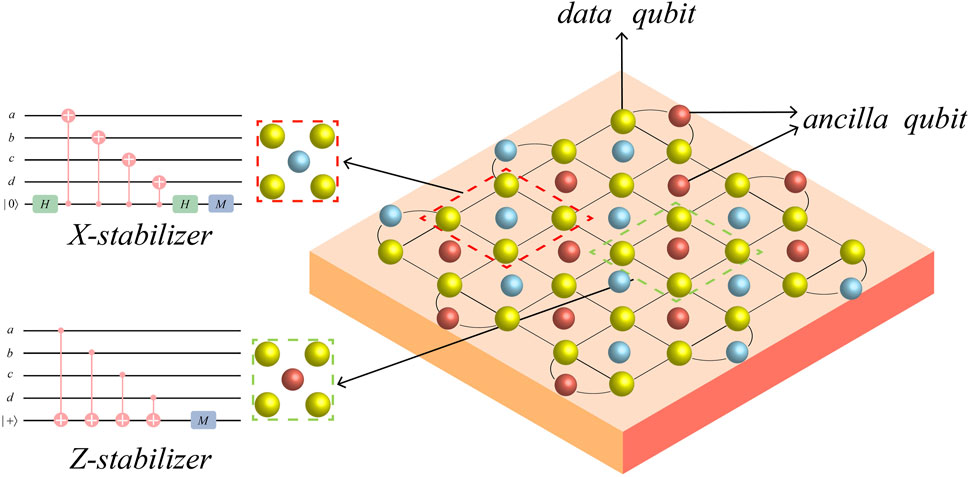
FIGURE 1. Rotated surface code with a code distance of 5. Each lattice vertex (yellow) is a data qubit. The orange (blue) in the figure is an ancilla qubit used for X(Z) stabilizer measurements. The quantum circuit for stabilizer measurements using Hadamard and CNOT gates is marked.

Specifically, in Figure 1, we associate the stabilizer generator with the color of ancilla qubits. The orange (blue) ancilla qubit forms an X(Z) stabilizer with the four (two) adjacent data qubits. We define the stabilizer as

$S_v=\otimes {\sigma }_v,v=\left\{x,z\right\}(4)$

and then define the logical X(Z) operator as X_L (Z_L).

2.2 Flag-bridge fault tolerance method

Flag qubits are used to monitor errors and notify other error-correcting qubits to perform error correction operations, while bridge qubits are used to connect error-correcting qubits and control qubits (used for executing quantum logical operations) at a closer physical distance, thereby improving the efficiency of error correction. The flag-bridge scheme exploits the existence of these ancilla qubits to more effectively control and reduce error propagation among quantum qubits, achieving more efficient FT quantum computing. Specifically, using flag and bridge qubits as ancilla qubits, additional information can be added to encoding information to detect and correct errors. This encoding method can be more easily implemented on near-term quantum processors and can be applied to various types of quantum errors. Flag and bridge qubits, as ancilla qubits, can improve the efficiency and accuracy of quantum error correction, providing new ideas for the practical application of near-term quantum computers.

Consider a stabilizer code $\mathcal{S}=⟨g_1,g_2,\dots ,g_r⟩$ and its QEC circuit $\mathcal{C}$ consisting of a flag-bridge circuit for measuring the stabilizer operator, i.e., $\mathcal{C}=\left\{c\left(g_1\right),c\left(g_2\right),\dots ,c\left(g_r\right)\right\}$, where $c\left(g_i\right)$ is the flag circuit for measuring the stabilizer g_i. We can check whether each circuit satisfies the fault tolerance condition by simulating it directly under circuit-level noise [26]. If two or more sets of errors lead to the same syndrome and flag string but no stabilizer is generated when multiplying them together, then the circuit is not FT.

As we described in Section 2.1, the weights of all stabilizer operators are either 2 or 4, regardless of the surface code lattice size. Therefore, the flag-bridge circuit applied to rotating surface codes requires at most four data qubits, as shown in Figure 2A. The circuit for measuring the Z-stabilizer with weight 4 is shown in Figure 2A. Only one more ancilla qubit is added by the flag-bridge approach in comparison to the preceding flag method. Each flag circuit behaves exactly like a non-FT circuit when there are no failures. When there is an error that appears and may affect subsequent circuits, it will generate a significant measurement of the flag qubits to be used to detect these errors. For example, if such an error occurs in the circuit in Figure 2A, it will not be FT; instead, if it occurs in the circuit shown in Figure 2B, the measurement of the qubit f will be 1, which means that a flag is raised [26].

FIGURE 2

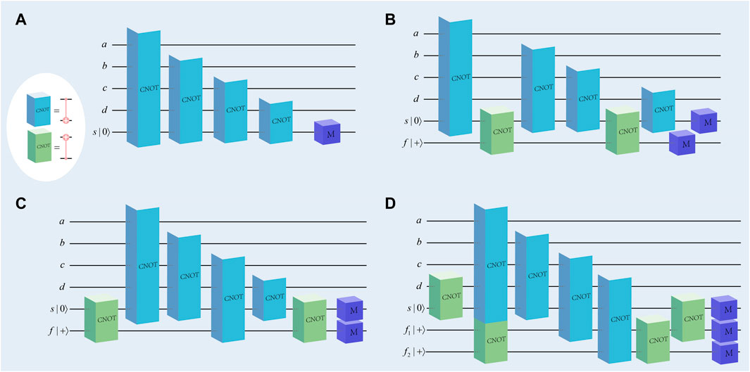
FIGURE 2. (A) The Z-stabilizer measurement circuit with a weight of 4. (B–D) Flag-bridge circuits (B, C) using two ancilla qubits and (D) using three ancilla qubits.

2.3 MBP₄ decoding of error codes

Given $R\in \mathcal{S}$ and a Pauli error E ∈ E_n, ER is referred to as a degenerate error of E since ER and E are equal on the code space. If there are stabilizers with weights smaller than the minimum distance of a quantum code, it is said to be degenerate; otherwise, it is non-degenerate.

Due to the ease with which a group of independent generators with weights $\le 4$ may be found, a surface code with d ≥ 5 is highly degenerate. In this work, we consider the quaternary quantum BP in log domain with an additional memory effect (MBP₄) [31]. A message passing technique called MBP₄, which makes use of the code’s degeneracy, is described by the check matrix of a code on the Tanner graph. A check matrix S of a code is an M × N matrix over error set E_n ∈ {I, X, Y, Z}, where M is the number of stabilizers that have been measured. For example, d = 7 rotated surface code has check matrix

$S=\left[\begin{array}{ccccccc}\hfill X\hfill & \hfill X\hfill & \hfill I\hfill & \hfill I\hfill & \hfill I\hfill & \hfill I\hfill & \hfill I\hfill \\ \hfill Z\hfill & \hfill I\hfill & \hfill I\hfill & \hfill Z\hfill & \hfill I\hfill & \hfill I\hfill & \hfill I\hfill \\ \hfill I\hfill & \hfill X\hfill & \hfill I\hfill & \hfill I\hfill & \hfill X\hfill & \hfill I\hfill & \hfill I\hfill \\ \hfill I\hfill & \hfill I\hfill & \hfill X\hfill & \hfill I\hfill & \hfill I\hfill & \hfill X\hfill & \hfill I\hfill \\ \hfill I\hfill & \hfill I\hfill & \hfill I\hfill & \hfill Z\hfill & \hfill I\hfill & \hfill I\hfill & \hfill Z\hfill \\ \hfill I\hfill & \hfill I\hfill & \hfill I\hfill & \hfill I\hfill & \hfill I\hfill & \hfill X\hfill & \hfill X\hfill \end{array}\right],$

and the corresponding Tanner graph, drawn as a factor graph to additionally display the initial distribution p_n, is shown in Figure 3.

FIGURE 3

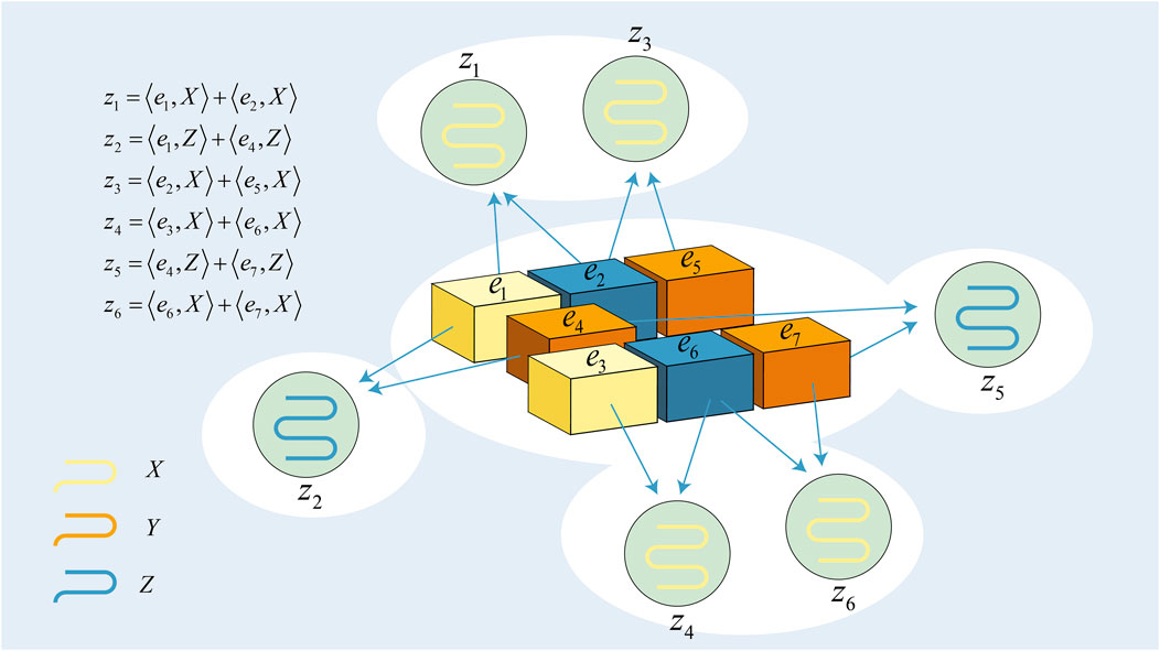
FIGURE 3. Tanner graph of d = 7 rotated surface code. e_i is a variable node with error. z_i is the syndrome.

3 Decoding with deep learning

3.1 Flag-bridge decoding

To demonstrate the operation of the flag-bridge circuit, we will utilize the circuit shown in Figure 2C. We designate the CNOT gate as the f-CNOT gate between the ancilla qubits and the s-CNOT gate between the data qubit and the ancilla qubit. As seen in Figure 2C, the ancilla qubits s and f are entangled through an s-CNOT gate (encoding circuit), and the stabilizer is represented as follows:

$⟨X_s\otimes X_f⟩,(5)$

and its corresponding logical operator is

$⟨X_L=X_s,Z_L=Z_s\otimes Z_f⟩.(6)$

This logical qubit is stabilized by X_L, after which stabilizer measurements are performed. Suppose there are four data qubits, denoted as (a, b, c, d), which are initially stabilized by (−1)^yZ_a,b,c,d, and the subsequent four s-CNOT gates will keep the stabilizer

$⟨X_s\otimes X_f,{\left(-1\right)}^y{Z}_{a,b,c,d}⟩(7)$

invariance of all qubits, but they gradually convert the logic operator to

$⟨X_L=X_s,Z_L=Z_s\otimes Z_f\otimes {\left(-1\right)}^y{Z}_{a,b,c,d}⟩.(8)$

Specifically, k_s and k_f s-CNOT gates can be applied to ancilla qubits s and f, respectively, where

$k_s+k_f=4,k_s,k_f\in Z.(9)$

For example, in Figure 2C, k_s = 2 and k_f = 2 [26]. After that, the last f-CNOT (decoding circuit) unravels so that the final stabilizer will consist of these two ancillas

$⟨{\left(-1\right)}^y{Z}_{a,b,c,d}⟩,(10)$

and the logical operators of these ancillas

$⟨X_f,{\left(-1\right)}^y{Z}_s⟩.(11)$

This means that the reading y measured on the ancilla s for M_z represents the measurement of the stabilizer Z_a,b,c,d. Thus, the circuit does measure the Z-check with weight 4. In addition, the measurement of the ancilla f implies the syndromes of the code; that is, it can detect a single Z-error occurring on any ancilla device and then raise a flag [26].

The following definition can be used to describe the flag-bridge method’s whole FT corrective cycle (Algorithm 1).

Algorithm 1. Flag-bridge scheme.

Input: Syndrome extraction circuit $c\left(g_i\right)\in \mathcal{C}$

1:  Initialize syndrome extraction circuit $c\left(g_i\right)\in \mathcal{C}$

     2:  F_i = number of flag entities in each circuit

3:  S_i = number of syndrome entities in each circuit

4:  for all (F_i, S_i) ∈ first round do

5:   if ∃ non-trivial $F_i^1$ or $S_i^1$ then

6:    break

7:   end if

8:  end for

9:  Perform second round, collect $F^2=U_i{F}_i^2$ and $S^2=U_i{S}_i^2$

10:  if $F_i^1$ is not empty then

     11:   use $F_i^1$ and S² (and F²)

12:  else if $F_i^1$ is empty, but $S_i^2$ is not empty then

13:   use S² (and F²)

14:  end if

3.2 Network architecture

Given that the look-up table decoder strategy is non-scalable, it would be ideal to have a scalable and quick decoding scheme that, when combined with the deep neural network approach, can achieve better results. The time complexity of classical algorithms grows exponentially with the size of the surface code. In contrast, the deep neural network decoder uses multiple layers of nonlinear transformations to model the complex relationship of surface codes, which can better learn nonlinear functions and, thus, improve decoding quality. In practice, deep neural network decoders can improve the performance of the decoder by increasing the network depth and width. In addition, the deep neural network decoder can adaptively adjust the model parameters to suit the structure and noise characteristics of different quantum surface codes. However, the traditional decoder needs to manually adjust the parameters of the decoding algorithm, which is not flexible enough. Deep neural network decoders can also use multi-task learning to simultaneously handle different decoding tasks, such as decoding different noise models or handling different surface code topologies. This multi-task learning can improve the generalization ability and scalability of the model. Therefore, the deep neural network decoder is more scalable than traditional decoders and can better solve the quantum surface code decoding problem.

The recovery operator R_z based on the syndrome z can be expressed as

$R_z=L\left(z\right)T\left(z\right)G\left(z\right)(12)$

and is called the LST decomposition of E [32]. In Eq. 12, L(z) is the product of logical operators, T(z) is the product of pure errors, and G(z) is the product of stabilizers. It should be noted that since the G(z) operator represents the stabilizer product, its choice does not affect the outcome of the recovery state. Therefore, given a measured syndrome z, our goal is to find the most probable logical operator in the non-trivial operator, denoted L(z), and then use L(z) to decode. The goal of the neural network is to find the most probable operator L(z) from the input syndrome z. All the codes we consider encode a single logical qubit; so, Eq. 12 can be rewritten as follows:

$R_z=X_L^{b_1\left(z\right)}{Z}_L^{b_2\left(z\right)}T\left(z\right)G\left(z\right),\left\{b_1\left(z\right),b_2\left(z\right)\in Z_2\right\}.(13)$

All syndromes were recorded following the conclusion of the two-round marker bridge syndrome extraction circuit. Given the error E and the syndrome z(E) = z (usually E will not know), the neural network must find the vector $b=\left(b_1(z),b_2(z)\right)$ such that $X_L^{b_1(z)}{Z}_L^{b_2(z)}{R}_{z}E\in \mathcal{S}$, where R_z is the original recovery operator obtained from the simple decoder.

We present our decoding strategy in Figure 4. The decoding strategy includes two module methods, the simple decoder and a DND. The purpose of using a DND is to improve the decoding performance of the simple decoder. In the depolarization error model, the correction provided by a simple decoder will result in an error-free logic state (I), approximately 42% of the time [33]. In this case, the neural network will output the identity operator (b in Figure 4). We will now describe our decoding strategy in detail. The first step is to use the flag-bridge method described in Section 2.2 to fault-tolerantly extract flags and error syndromes information to generate dataset information. Then, the simple decoder and DND will analyze and judge the dataset in a distributed manner. A simple decoder will correct for partial error syndrome, and the DND will predict from the dataset whether or not it will cause a logical error (I, X, Y, Z), and its expected output is a binary value indicating whether extra correction needs to be applied. The dataset is finally corrected by combining the prediction results of the simple decoder and DND to achieve a high accuracy rate.

FIGURE 4

FIGURE 4. Description of the design of the DND decoder.

3.3 Training

The syndromes and flags from both rounds will be gathered in the input stages when employing the flag-bridge error correction. Therefore, the input layer should contain information about both rounds of syndromes and flags. For better application to the convolutional neural network, we embed the L = d code lattice into a (2L + 1) × (2L + 1) binary matrix. We encode error syndromes and sign messages in this way. The total input can be obtained by stacking the flag pieces on top of the error syndrome pieces, thus effectively creating inputs suitable for use as a convolutional neural network. The feed-forward neural network is stacked on top of several convolutional layers to create the deep neural network that we utilize. Fully connected feed-forward layers follow the convolutional layers, and we use ReLU [34] as the activation function for the hidden layer and softmax as the activation function for the output layer. The error syndrome is passed through a series of convolutional layers of decreasing size (from (2L + 1) × (2L + 1) to 2 × 2), each with 64 output filters, followed by a fully connected layer with 512 neurons, and then in decoder labels. To quicken the model’s training process and make sure the model can successfully learn more extensive datasets, ResNet [35] network layers were introduced as the underlying architecture, ensuring that the shortcut output is added to the output of the stacking layers through the remaining blocks, and data are stacked using ResNet 7, 14, and 21 network layers. Training allows for a large amount of stacking without degrading the learning efficiency of the convolutional layers. Additionally, the feed-forward neural network’s fully connected network parameters and the convolutional neural network parameters must be regularly synchronized to maintain data integrity.

Training starts with the input syndromes and flags data; the input layer receives syndromes and flags information, and the output layer ideally should encapsulate any logical mistakes caused by the auxiliary decoding algorithm in the target output. The objective is to use the DND to forecast these logical mistakes, and when it does, we apply a logic Pauli operator following the recovery recommended by the auxiliary decoder. To train the DND decoder, we use one-hot encoding to represent the decoder labels and binary cross-entropy loss as the training objective. This design is enough to convey the power of our paradigm while avoiding further complexity.

Algorithm 2. Network training.

Input: $D={\left\{({\mathbf{x}}_k,{\mathbf{y}}_k)\right\}}_{k=1}^m$; learning rate η

Output: One-hot encoding label

1:  Embed L = d code lattice into a (2L + 1) × (2L + 1) binary matrix

2:  Initialize training set $D={\left\{({\mathbf{x}}_k,{\mathbf{y}}_k)\right\}}_{k=1}^m\leftarrow$ flag-bidge scheme

3:  Randomly initialize all connection weights in the network in the range (0,1)

4:  repeat

5:   for all (x_k, y_k) ∈ D do

6:    Compute the current sample output ${\widehat{\mathbf{y}}}_k=f({\beta }_j-{\theta }_j)$

7:    Calculate the gradient of the output neuron g_i

8:    Compute the neuron gradient term for the hidden layer e_h

9:    Update weights $\begin{array}{cc}\hfill \mathrm{\Delta }{w}_{hj}& =\eta g_j{b}_h\hfill \\ \hfill \mathrm{\Delta }{v}_{ih}& =\eta e_h{x}_i\hfill \end{array}$

10:   end for

11:  until stop condition reached

12:  Return one-hot

Convolutional neural networks consist of two steps in their training process. The forward propagation phase, also referred to as the first phase, is when data are sent from the lower level to the upper level. The second stage, or the backward propagation stage, occurs when the outcome of forward propagation does not match the expectation and the mistake is transmitted from the higher level to the lower level for training. The training process initializes the network weights. The training is completed when the error is equal to or less than the desired level of accuracy [36].

Specifically, in Figure 5, we describe how the neural network we used was trained. In the first step, we encode the flag and error syndrome information into a binary matrix of size (2L + 1) × (2L + 1) to better fit the input of the convolutional layer. The orange and green matrices consist of error syndrome and flag information, respectively. The second step is to change the network weights initially. The input data are forwarded through the convolutional layer, the downsampling layer, and the fully connected layer to obtain the output value (i.e., the forward propagation stage in Figure 5). In this work, we did this by chaining a feed-forward neural network after a convolutional neural network. After the feed-forward neural network, we get the output (represented as the green block one-hot encoded label in Figure 5). After the third step, the error is obtained by comparing the output value with the target value, and the weights are optimized according to the error. Algorithm 2 shows the pseudo-code form of the training phase.

FIGURE 5

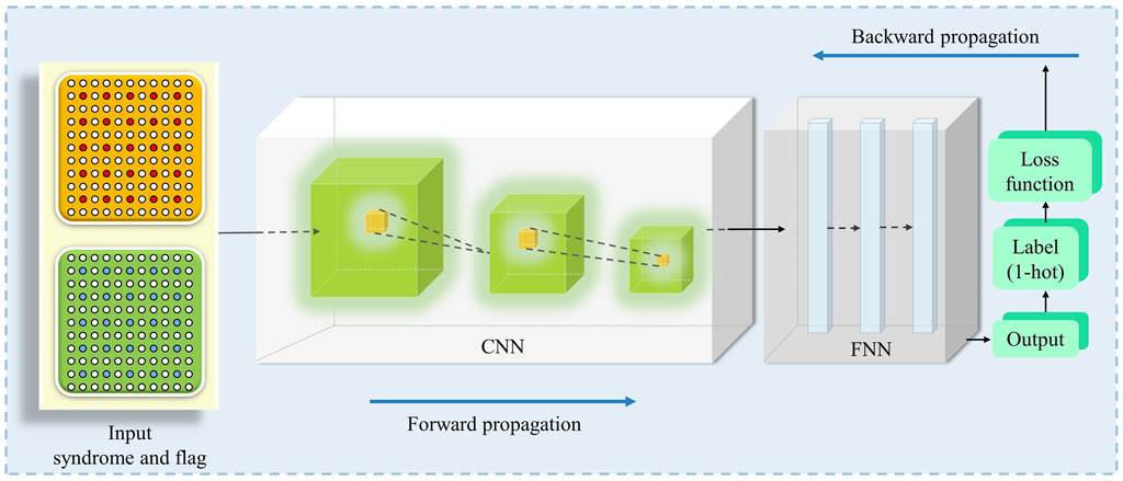
FIGURE 5. Details of the DND decoding used for the L × L code grid. Individual fault syndromes are embedded in a (2L + 1) × (2L + 1) binary matrix with all entries initially set to 0 by default. Entries indicated by red circles are set to −1 to show the offending syndrome, and entries indicated by blue circles are flag information. By overlaying syndromes and flag slices, the input data can be created in a way that is appropriate for convolutional neural network input. We stacked a feed-forward neural network on top of the convolutional layer, and the final output was one-hot coded.

4 Decoding with MBP₄ as an RNN

4.1 Models and algorithms

A quaternary $\mathrm{B}\mathrm{P}\left({\mathrm{B}\mathrm{P}}_4\right)$ algorithm computes an approximated marginal distribution $P\left(e_n=w\mid z\right)=q_n^w$, where w ∈ {I, X, Y, Z} indicates the error type, n = 1, 2, … , N in linear domain [23], and outputs $\widehat{e}=\left({\widehat{e}}_1,{\widehat{e}}_2,\dots ,{\widehat{e}}_N\right)$ such that

${\widehat{e}}_n=\underset{w}{\arg \max }P\left(e_n=w\mid z\right).$

As an alternative, the log-likelihood ratio (LLR) of the form can be used

${\mathrm{\Gamma }}_n^X=\ln \frac{q_n^I}{q_n^X},{\mathrm{\Gamma }}_n^Y=\ln \frac{q_n^I}{q_n^Y},{\mathrm{\Gamma }}_n^Z=\ln \frac{q_n^I}{q_n^Z}$

in log domain [37]. The decoder will output $\widehat{e}$ if the syndrome of $\widehat{e}$ matches z.

BP₄ is given in log domain with an LLR vector $\mathrm{\Gamma }=\left({\mathrm{\Gamma }}_1,{\mathrm{\Gamma }}_2,\dots ,{\mathrm{\Gamma }}_N\right)\in R^{3N}$, where

${\mathrm{\Gamma }}_n=\left({\mathrm{\Gamma }}_n^X,{\mathrm{\Gamma }}_n^Y,{\mathrm{\Gamma }}_n^Z\right)\in R^{3}n=\mathrm{1,2},\dots ,N.$

On each edge (m, n) linking variable node n and check node m, two different sorts of messages are iteratively transmitted. Let M(n) denote the set of variable nodes n nearby check nodes and N(m) denote the set of check nodes m nearby variable nodes [23]. A variable-to-check message is displayed using ${\lambda }_{S_{mn}}\left({\mathrm{\Gamma }}_{n\to m}\right)$ that contains the LLR that E_n commutes or anticommutes with S_mn from variable node n to check node m, where ${\mathrm{\Gamma }}_{n\to m}=\left({\mathrm{\Gamma }}_{n\to m}^X,{\mathrm{\Gamma }}_{n\to m}^Y,{\mathrm{\Gamma }}_{n\to m}^Z\right)$ is the LLR of e_n = w, according to the messages from the other nodes m′ ∈ M(n)\m, and the function λ_w: R³ → R is defined as follows

${\lambda }_w\left(x,y,z\right)\triangleq \ln \frac{1+e^{-\omega }}{e^{-x}+e^{-y}+e^{-z}-e^{-\omega }}.$

The LLR of whether e_n commutes or anticommutes with S_mn is, therefore, revealed by a check-to-variable message Δ_m→n from check node m to variable node n. More specifically,

${\mathrm{\Delta }}_{m\to n}={\left(-1\right)}^{z_m}\underset{n^{\prime }}{⊞}{\lambda }_{S_{m{n}^{\prime }}}\left({\mathrm{\Gamma }}_{n^{\prime }\to m}\right),$

where for a set of k real scalars a₁, a₂, … , a_k ∈ R, the operation ⊞ is defined by

${\displaystyle \underset{n=1}{k}}{a}_n=2{\tanh }^{-1}\left({\displaystyle \prod _{n=1}^k}\tanh \frac{a_n}{2}\right).$

Then, Γ_n is updated according to Δ_m→n for all m ∈ M(n) and the initial distribution of e_n.

The BP algorithm iteratively updates the LLR of the marginal distributions ${\left\{{\mathrm{\Gamma }}_n\right\}}_{n=1}^N$ according to the passed messages on the Tanner graph. A Tanner graph, which is a bipartite graph with variable nodes and checks nodes connected appropriately by edges, may be used to represent the parity-check matrix of a code. The BP algorithm on the Tanner graph sends messages between the nodes iteratively in order to obtain an estimate of the marginal distribution for each coordinate of the error.

Consider an M × N check matrix S. A Tanner graph that has M check nodes (corresponding to the given binary syndrome vector) and N variable nodes (corresponding to the N-fold Pauli error to be estimated) can be used to represent the relationships between a Pauli error operator and its syndrome bits. Variable node n and check node m are connected by S_mn whenever I ≠ S_mn ∈ {X, Y, Z}. Figure 6 illustrates the Tanner graph for a check matrix $S=\left[\begin{array}{ccc}\hfill X\hfill & \hfill Y\hfill & \hfill I\hfill \\ \hfill Z\hfill & \hfill Z\hfill & \hfill Y\hfill \end{array}\right]$.

FIGURE 6

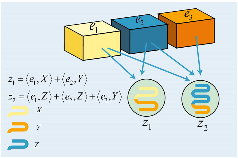
FIGURE 6. Tanner graph for S. There are three variable nodes (represented by circles) and two check nodes (represented by squares).

Considering degenerate quantum codes; for all the check nodes, we use two unifying parameters a⁻¹, b ∈ R in MBP₄. At the beginning of MBP₄, for check matrix S, let

${\mathrm{\Gamma }}_{n\to m}^w={\mathrm{\Lambda }}_n^w,(14)$

where ${\mathrm{\Gamma }}_{n\to m}^w$ is LLRs from variable node n to check node m and ${\mathrm{\Lambda }}_n^w$ is the channel statistics vector. We parallelly calculate check node m and variable node n horizontally and vertically, respectively. First, in the horizontal step, we compute

${\mathrm{\Delta }}_{m\to n}={\left(-1\right)}^{z_m}\underset{n^{\prime }}{⊞}{\lambda }_{S_{m{n}^{\prime }}}\left({\mathrm{\Gamma }}_{n^{\prime }\to m}\right),(15)$

where Δ_m→n means the check-to-variable message and ${\lambda }_{S_{m{n}^{\prime }}}\left({\mathrm{\Gamma }}_{n^{\prime }\to m}\right)$ means the variable-to-check message. Furthermore, in the vertical step, we compute

$\begin{array}{c}\hfill {\mathrm{\Gamma }}_n^w={\mathrm{\Lambda }}_n^w+\frac{1}{a}{\displaystyle \sum _{\begin{array}{c}⟨w,S_{mn}⟩=1\end{array}}}{\mathrm{\Delta }}_{m\to n}-b{\displaystyle \sum _{\begin{array}{c}{S}_{mn}=w\end{array}}}{\mathrm{\Delta }}_{m\to n}\end{array}.(16)$

Then, we have a hard decision. Let $\widehat{e}={\widehat{e}}_1{\widehat{e}}_2\cdots {\widehat{e}}_N$, ${\widehat{e}}_n=I$ if ${\mathrm{\Gamma }}_n^w>0$ and ${\widehat{e}}_n=\underset{w\in \{X,Y,Z\}}{\mathrm{arg\; min}}{\mathrm{\Gamma }}_n^w$, otherwise. At this time, for ∀m, if $⟨\widehat{e},S_m⟩=z_m$, we say it is converge. If $⟨\widehat{e},S_m⟩\ne z_m$ or the maximum number of iterations T_max is reached, we say it is a fail. If any of the conditions are not met, we repeat all steps from the horizontal step. At the end of the algorithm, MBP₄ introduced a fixed inhibition, by computing

${\mathrm{\Gamma }}_{n\to m}^w={\mathrm{\Gamma }}_n^w-⟨w,S_{mn}⟩{\mathrm{\Delta }}_{m\to n}.(17)$

Equation (17) can be expressed in the following form:

$\begin{array}{cc}\hfill {\mathrm{\Gamma }}_{n\to m}^w& ={\mathrm{\Lambda }}_n^w+\frac{1}{a}{\displaystyle \sum _{\begin{array}{c}⟨w,S_{m^{\prime }n}⟩=1\end{array}}}{\mathrm{\Delta }}_{m^{\prime }\to n}-b{\displaystyle \sum _{\begin{array}{c}{S}_{m^{\prime }n}=w\end{array}}}{\mathrm{\Delta }}_{m^{\prime }\to n}\hfill \\ \hfill & -⟨w,S_{mn}⟩{\mathrm{\Delta }}_{m\to n}.\hfill \end{array}(18)$

The term $-⟨w,S_{mn}⟩{\mathrm{\Delta }}_{m\to n}$ is called inhibition [31], which provides adequate strength to resist a wrong belief looping in the short cycle. By maintaining such inhibition strength, decoding can be made less affected by the short cycles. Moreover, the term $-b{\sum }_{\begin{array}{c}{S}_{m^{\prime }n}=w\end{array}}{\mathrm{\Delta }}_{m^{\prime }\to n}$ is also like an inhibition. Since it is induced from gradient decent optimization, we simply have a step size b to adjust its strength. It has been proved that MBP₄ performs better with b = 0.

As far as we know, the decoding process of BP can be modeled as an RNN [38,39], which usually adopts a parallel scheduling scheme. For the RNN, and for simplicity and effect, we set b = 0. In the Tanner graph corresponding to the M × N check matrix S, there are two types of messages that are iteratively updated, namely, variable-to-check and check-to-variable messages. Therefore, there will be two hidden layers in the designed RNN, which alternately compute Δ_m→n or ${\lambda }_{S_{mn}}\left({\mathrm{\Gamma }}_{n\to m}\right)$ message, with N input neurons ${\left\{{\mathrm{\Lambda }}_n\right\}}_{n=1}^N$ and output neurons ${\left\{{\mathrm{\Gamma }}_n\right\}}_{n=1}^N$. The estimated error $\widehat{e}$ can be calculated from ${\left\{{\mathrm{\Gamma }}_n\right\}}_{n=1}^N$. The ultimate goal of the RNN is to find the most likely error $\widehat{e}$ for the syndrome z. It should be noted that the computation will also terminate if the maximum number of iterations T_max is reached.

Figure 7 illustrates the RNN designed on the basis of Figure 6. The neuron Γ_n→m computes ${\lambda }_{S_{mn}}\left({\mathrm{\Gamma }}_{n\to m}\right)$, from Δ_m→n to the dotted line between ${\lambda }_{S_{mn}}\left({\mathrm{\Gamma }}_{n\to m}\right)$ indicates suppression and each solid edge is an incentive.

FIGURE 7

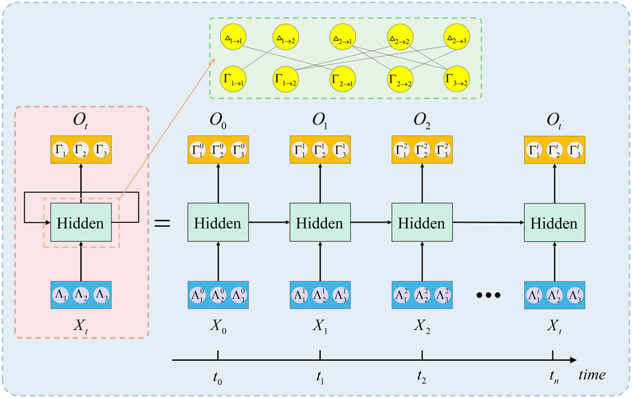
FIGURE 7. RNN designed on the basis of Figure 6; the two hidden layers alternately calculate Δ_m→n or ${\lambda }_{S_{mn}}\left({\mathrm{\Gamma }}_{n\to m}\right)$ messages on each edge, and there are N input neurons ${\left\{{\mathrm{\Lambda }}_n\right\}}_{n=1}^N$ and output neuron ${\left\{{\mathrm{\Gamma }}_n\right\}}_{n=1}^N$.

To sum up, we have shown that MBP₄ can be extended to a neural network decoder, which may be further improved by using appropriate weight α for each edge. We select the edge weight a by using the general optimization scheme of the neural network.

4.2 Decoding surface code

We provide an example of the decoding on the d = 7 surface code in Figures 8A–C.

FIGURE 8

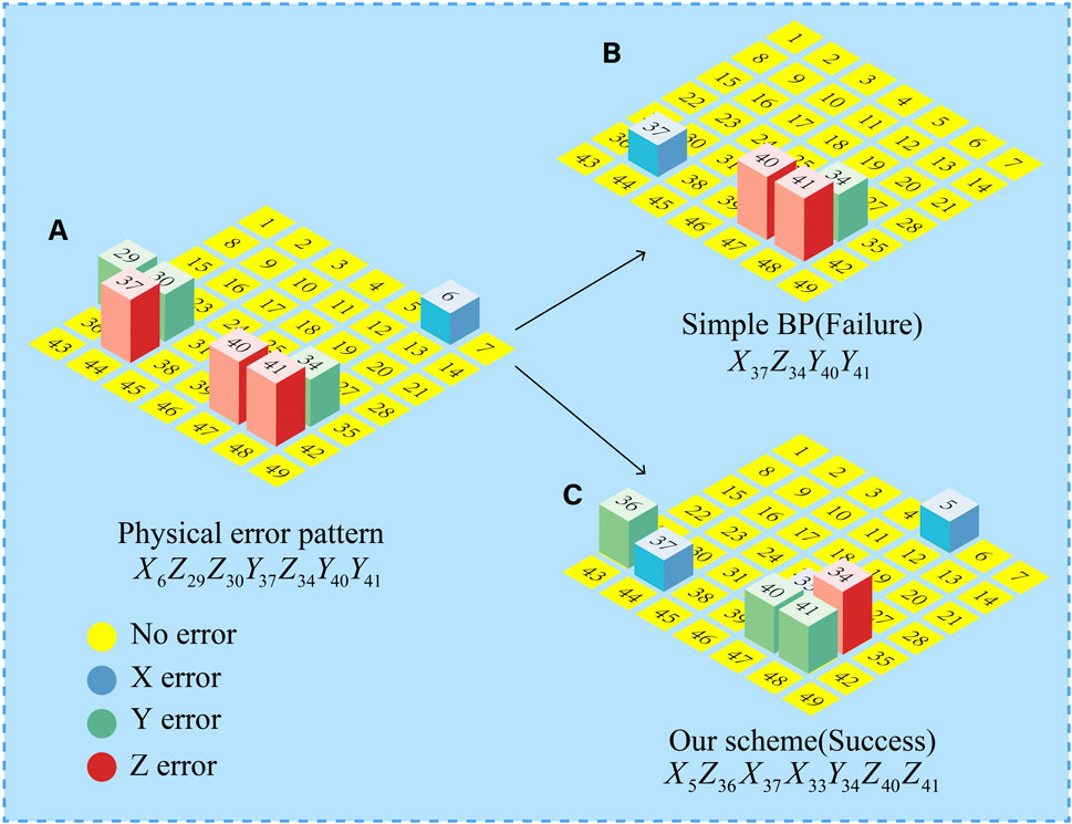
FIGURE 8. (A–C) Examples of a d = 7 surface code. Error-free quantum graduations are represented by numbered yellow circles. A blue, green, or red square column indicates a qubit with X-, Y-, or Z-error, respectively. (A) The actual error pattern. (B) The decoding result of the simple BP algorithm, when the decoding result has errors that do not match the syndrome. (C) The RNN decoding process of MBP₄.

Figure 8A depicts the error with a weight of 7. The error X on qubit 6 is anticommutated with the stabilizer Z₅Z₆Z₁₂Z₁₃, so the corresponding syndrome bit is 1. The simple BP algorithm cannot determine whether the error X is on qubit 5 or qubit 6. In order to overcome this symmetry, post-processing or pre-processing can be chosen. Since we use the RNN model designed by MBP₄ for decoding, we take a post-processing method, which will determine that the error X occurs in qubit 5. Post-processing has two steps. The first step is to remove surface complexity from the lattice. Whenever the error approximation distribution p_e > 0.5 [15], we apply the appropriate error correction operation on the error lattice and switch p_e to its original value. While neural networks can learn to do the same thing, it is often very expensive. The second step is to concretize. The most likely error location can be found by approximating the distribution.

Now, we consider the complete set of errors on the surface code in Figure 8A. The RNN scheme performs fast asymmetric updates with large strides. It performs a very aggressive search without jumping erroneously, finally converging to a valid degenerate error. Figure 8C depicts all the errors identified. The error in Figure 8C is equivalent to the error in Figure 8A, up to three stabilizers X₅X₆, Z₂₉Z₃₀Z₃₆Z₃₇ and X₃₃X₃₄X₄₀X₄₁.

5 Numerical experiments and analysis

5.1 Performance analysis

The corresponding circuits were simulated, first using the flag-bridge syndrome extraction circuit so that syndromes and flags were included in the dataset. The size of the training set was chosen according to the size of the code distance. For d = 3, d = 5, and d = 7, the size of the dataset was set to 2 × 10⁶, 2 × 10⁷, and 2 × 10⁸, respectively. In the design of the training set, we used 95% as the training data, and the remaining 5% was used as the test set to test the actual learning ability of the network. We tested our integrated decoder on these data and assessed its logical error rate compared to the MWPM decoder.

Figure 9 depicts a graph of the logical error rate and physical error rate. When using our decoder, the error correction success rate was greatly improved. The dashed line y = x intersecting each decoder indicates the pseudo-threshold [40]. The results show that the pseudo-threshold of the surface codes was improved when using our decoder. For example, Figure 9A illustrates an improvement in the pseudo-threshold of 39.52% for the d = 3 surface code.

FIGURE 9

FIGURE 9. Rotating surface codes are decoded using MWPM and a DND, and the values represent pseudo-threshold values. (A) d = 3. (B) d = 5. (C) d = 7.

The decoding performance and decoder threshold of the two decoders are illustrated in Figures 10A, B, and we illustrate the decoder performance with MLD in Figure 10C. In order to study the impact of a larger code distance, we increased the distance to 13, and the surface codes correspond to the code distance of d = 9, 11, 13 using the DND decoders that are described in Figure 10A. In the figure, the intersection of the yellow dashed line and three curves represents the decoder threshold, and a decoding threshold of about 15.8% can be observed. This is higher than the 15.5% [41] achieved by the previous MWPM decoding algorithm.

FIGURE 10

FIGURE 10. Decoding performance of d = 9, 11, 13 rotated surface codes; the intersection represents threshold. (A) Decoding using a DND. (B) Decoding using an RNN of MBP₄. (C) Decoding using MLD.

The decoding threshold can be observed in Figure 10B. Through the iterative calculation and optimization of the RNN, the edge weight α was determined between {1, 0.99, … , 0.5}, but because the RNN we used has an inhibitory effect, it also includes the existence of edges with a weight of −1, which can enhance the performance of the RNN. By using the weight combination of a = 0.65 and a = −1, the performance curve of the decoder is as shown in Figure 10B. Since surface codes with larger distances have better degeneracy, we extended the code distance to 13 in the figure to better demonstrate the decoding performance. The dotted line in the figure represents no error correction. About 16.4% of the decoder threshold performance can be observed in Figure 10B. Compared with the DND decoding scheme, this scheme has better decoding performance. Furthermore, we also illustrate the decoding performance curve with MLD in Figure 10C. During the decoding process of MLD, the maximum likelihood decoder will first establish a probability model. This model describes the relationship between the received codewords and the codewords actually sent by all possible senders and uses statistical methods to estimate model parameters, such as the mean and variance of the error distribution. Next, the maximum likelihood decoder calculates the distance or difference between each possible codeword and the received codeword and converts this into a probability value. Specifically, it calculates the probability of each possible codeword generating the received codeword based on the model parameters and chooses the one that minimizes the distance or difference between the received codeword and the codeword actually sent by the sender. The codeword is used as the decoding result. Although, in general, the effect of MLD is better than that of MWPM. However, MLD needs to calculate all possible error modes and select the mode with the highest probability as the decoding result. The time complexity of this process is very high. As the system scale increases sharply, it becomes difficult to achieve practical applications. In contrast, our scheme is faster, easier to implement, and more practical than MLD when dealing with larger-scale quantum surface codes. By observing Figure 10C, we can find that the threshold of MLD is slightly lower than that of our scheme.

5.2 The cost of a decoder

The cost of a QEC decoder can vary depending on the specific algorithm used and the hardware platform it is implemented on. In general, decoding algorithms for QEC can require significant computational resources, which can translate to increased hardware and energy costs. In addition to the threshold, the cost can also be considered as a measure of decoder quality because a more efficient and cost-effective decoder can make QEC more practical and scalable for real-world quantum computing applications.

In our deep neural network decoder scheme, the cost of the decoder depends on various factors, such as the specific architecture of the neural network, the size of the surface code, and the hardware platform used for training and inference. Specifically, GPUs or TPUs are required for training neural networks. Additionally, the time and effort spent on training the neural network in terms of surface code size should also be considered.

6 Conclusion

It is difficult to find effective decoders that are appropriate for quantum error-correcting codes for FT experiments. In this article, based on the flag-bridge fault tolerance experiment, we studied two decoding strategies. The first scheme used the deep learning method to improve the original decoding process based on the flag-bridge method and we added a simple decoder to it to cooperate with the neural network decoding work. The simple decoder that replaced the look-up table decoder in the original flag-bridge method allows for better scalability. Compared with the MWPM decoder, the pseudo-threshold of our decoding scheme was improved by 39.52%, and it can reach a decoder threshold of approximately 15.8%. The second scheme used the MBP₄ algorithm to design the RNN structure and used the post-processing method to achieve better decoding performance than the deep neural network decoding scheme. Our approach also has the potential for LDPC codes. For instance, in [39], a neural network was combined with the traditional BP algorithm and the neural network’s nonlinear characteristics were utilized to improve the accuracy and speed of error correction. The neural BP decoder was successfully applied to quantum LDPC codes. Our work is based on the improvement of the BP algorithm and neural network. Therefore, our decoder has potential when applied to quantum LDPC codes. Stable mistakes are another factor that mature neural network decoders must consider. However, our training process does not take this into account, and the training accuracy was far from sufficient. More importantly, our scheme can only meet the fault tolerance of small experiments. In the future, we need to find the conditions that meet the fault tolerance experiments of large-distance codes to realize fault tolerance and correction better.

Data availability statement

The raw data supporting the conclusion of this article will be made available by the authors, without undue reservation.

Author contributions

NJ: conceptualization, methodology, and software; ZC: data curation and writing—original manuscript preparation; YQ: visualization, investigation, and supervision; RB: writing—reviewing and editing; XY: funding acquisition and resources; and SW: conceptualization, funding acquisition, and resources. All authors contributed to the article and approved the submitted version

Funding

This project was supported by the National Natural Science Foundation of China (Grant No. 42201506), Natural Science Foundation of Shandong Province, China (Grant No. ZR2021MF049), Joint Fund of the Natural Science Foundation of Shandong Province (Grant No. ZR2022LLZ012), and Joint Fund of the Natural Science Foundation of Shandong Province (Grant No. ZR2021LLZ001).

Conflict of interest

The authors declare that the research was conducted in the absence of any commercial or financial relationships that could be construed as a potential conflict of interest.

Publisher’s note

All claims expressed in this article are solely those of the authors and do not necessarily represent those of their affiliated organizations, or those of the publisher, the editors, and the reviewers. Any product that may be evaluated in this article, or claim that may be made by its manufacturer, is not guaranteed or endorsed by the publisher.

References

1. Knill E, Laflamme R. Theory of quantum error-correcting codes. Phys Rev A (1997) 55:900–11. doi:10.1103/physreva.55.900

CrossRef Full Text | Google Scholar

2. Kitaev AY. Fault-tolerant quantum computation by anyons. Ann Phys (2003) 303:2–30. doi:10.1016/s0003-4916(02)00018-0

CrossRef Full Text | Google Scholar

3. Shors P. Scheme for reducing decoherence in quantum computer memory. Phys Rev A (1995) 52:2493–6. doi:10.1103/physreva.52.r2493

PubMed Abstract | CrossRef Full Text | Google Scholar

4. Steane AM. Active stabilization, quantum computation, and quantum state synthesis. Phys Rev Lett (1997) 78:2252–5. doi:10.1103/physrevlett.78.2252

CrossRef Full Text | Google Scholar

5. Dennis E, Kitaev A, Landahl A, Preskill J. Topological quantum memory. J Math Phys (2002) 43:4452–505. doi:10.1063/1.1499754

CrossRef Full Text | Google Scholar

6. Bombín H. An introduction to topological quantum codes. arXiv preprint arXiv:1311.0277 (2013).

Google Scholar

7. Kolmogorov V. Blossom v: A new implementation of a minimum cost perfect matching algorithm. Math Programming Comput (2009) 1:43–67. doi:10.1007/s12532-009-0002-8

CrossRef Full Text | Google Scholar

8. Bravyi S, Suchara M, Vargo A. Efficient algorithms for maximum likelihood decoding in the surface code. Phys Rev A (2014) 90:032326. doi:10.1103/physreva.90.032326

CrossRef Full Text | Google Scholar

9. Duclos-Cianci G, Poulin D. Fast decoders for topological quantum codes. Phys Rev Lett (2010) 104:050504. doi:10.1103/physrevlett.104.050504

PubMed Abstract | CrossRef Full Text | Google Scholar

10. Cook W, Rohe A. Computing minimum-weight perfect matchings. INFORMS J Comput (1999) 11:138–48. doi:10.1287/ijoc.11.2.138

CrossRef Full Text | Google Scholar

11. Torlai G, Melko RG. Neural decoder for topological codes. Phys Rev Lett (2017) 119:030501. doi:10.1103/physrevlett.119.030501

PubMed Abstract | CrossRef Full Text | Google Scholar

12. Varsamopoulos S, Criger B, Bertels K. Decoding small surface codes with feedforward neural networks. Quan Sci Tech (2017) 3:015004. doi:10.1088/2058-9565/aa955a

CrossRef Full Text | Google Scholar

13. Chamberland C, Ronagh P. Deep neural decoders for near term fault-tolerant experiments. Quan Sci Tech (2018) 3:044002. doi:10.1088/2058-9565/aad1f7

CrossRef Full Text | Google Scholar

14. Sweke R, Kesselring MS, van Nieuwenburg EP, Eisert J. Reinforcement learning decoders for fault-tolerant quantum computation. Machine Learn Sci Tech (2020) 2:025005. doi:10.1088/2632-2153/abc609

CrossRef Full Text | Google Scholar

15. Ni X. Neural network decoders for large-distance 2d toric codes. Quantum (2020) 4:310. doi:10.22331/q-2020-08-24-310

CrossRef Full Text | Google Scholar

16. Wang H-W, Xue Y-J, Ma Y-L, Hua N, Ma H-Y. Determination of quantum toric error correction code threshold using convolutional neural network decoders. Chin Phys B (2021) 31:010303. doi:10.1088/1674-1056/ac11e3

CrossRef Full Text | Google Scholar

17. Xue Y-J, Wang H-W, Tian Y-B, Wang Y-N, Wang Y-X, Wang S-M. Quantum information protection scheme based on reinforcement learning for periodic surface codes. Quan Eng (2022) 2022:1–9. doi:10.1155/2022/7643871

CrossRef Full Text | Google Scholar

18. Baireuther P, O’Brien TE, Tarasinski B, Beenakker CW. Machine-learning-assisted correction of correlated qubit errors in a topological code. Quantum (2018) 2:48. doi:10.22331/q-2018-01-29-48

CrossRef Full Text | Google Scholar

19. Baireuther P, Caio MD, Criger B, Beenakker CW, O’Brien TE, Neural network decoder for topological color codes with circuit level noise. New J Phys (2019) 21:013003. doi:10.1088/1367-2630/aaf29e

CrossRef Full Text | Google Scholar

20. Bishop CM, Nasrabadi NM. Pattern recognition and machine learning. Germany: Springer (2006).

Google Scholar

21. Goodfellow I, Bengio Y, Courville A. Deep learning. Cambridge: MIT press (2016).

Google Scholar

22. Kuo K-Y, Lai C-Y. Refined belief propagation decoding of sparse-graph quantum codes. IEEE J Selected Areas Inf Theor (2020) 1:487–98. doi:10.1109/jsait.2020.3011758

CrossRef Full Text | Google Scholar

23. Yan D-D, Fan X-K, Chen Z-Y, Ma H-Y. Low-loss belief propagation decoder with tanner graph in quantum error-correction codes. Chin Phys B (2022) 31:010304. doi:10.1088/1674-1056/ac11cf

CrossRef Full Text | Google Scholar

24. Chamberland C, Beverland ME. Flag fault-tolerant error correction with arbitrary distance codes. Quantum (2018) 2:53. doi:10.22331/q-2018-02-08-53

CrossRef Full Text | Google Scholar

25. Chao R, Reichardt BW. Flag fault-tolerant error correction for any stabilizer code. PRX Quan (2020) 1:010302. doi:10.1103/prxquantum.1.010302

CrossRef Full Text | Google Scholar

26. Lao L, Almudever CG. Fault-tolerant quantum error correction on near-term quantum processors using flag and bridge qubits. Phys Rev A (2020) 101:032333. doi:10.1103/physreva.101.032333

CrossRef Full Text | Google Scholar

27. Gottesman D. Stabilizer codes and quantum error correction. California: California Institute of Technology (1997).

Google Scholar

28. Calderbank AR, Rains EM, Shor P, Sloane NJ. Quantum error correction via codes over gf (4). IEEE Trans Inf Theor (1998) 44:1369–87. doi:10.1109/18.681315

CrossRef Full Text | Google Scholar

29. Horsman C, Fowler AG, Devitt S, Van Meter R. Surface code quantum computing by lattice surgery. New J Phys (2012) 14:123011. doi:10.1088/1367-2630/14/12/123011

CrossRef Full Text | Google Scholar

30. Tomita Y, Svore KM. Low-distance surface codes under realistic quantum noise. Phys Rev A (2014) 90:062320. doi:10.1103/physreva.90.062320

CrossRef Full Text | Google Scholar

31. Kuo K-Y, Lai C-Y. Exploiting degeneracy in belief propagation decoding of quantum codes. npj Quan Inf (2022) 8:111–9. doi:10.1038/s41534-022-00623-2

CrossRef Full Text | Google Scholar

32. Qin Z-H, Wang F. An effective method for lst decomposition based on the linear spectral mixing model. J lnfrared Millimeter Waves (2015) 34:497.

Google Scholar

33. Varsamopoulos S, Bertels K, Almudever CG. Decoding surface code with a distributed neural network–based decoder. Quan Machine Intelligence (2020) 2:3–12. doi:10.1007/s42484-020-00015-9

CrossRef Full Text | Google Scholar

34. Agarap AF. Deep learning using rectified linear units (relu). arXiv preprint arXiv:1803.08375 (2018).

Google Scholar

35. Targ S, Almeida D, Lyman K. Resnet in resnet: Generalizing residual architectures. arXiv preprint arXiv:1603.08029 (2016).

Google Scholar

36. O’Shea K, Nash R. An introduction to convolutional neural networks. arXiv preprint arXiv:1511.08458 (2015).

Google Scholar

37. Lai C-Y, Kuo K-Y. Log-domain decoding of quantum ldpc codes over binary finite fields. IEEE Trans Quan Eng (2021) 2:1–15. doi:10.1109/tqe.2021.3113936

CrossRef Full Text | Google Scholar

38. Nachmani E, Marciano E, Lugosch L, Gross WJ, Burshtein D, Be’ery Y. Deep learning methods for improved decoding of linear codes. IEEE J Selected Top Signal Process (2018) 12:119–31. doi:10.1109/jstsp.2017.2788405

CrossRef Full Text | Google Scholar

39. Liu Y-H, Poulin D. Neural belief-propagation decoders for quantum error-correcting codes. Phys Rev Lett (2019) 122:200501. doi:10.1103/physrevlett.122.200501

PubMed Abstract | CrossRef Full Text | Google Scholar

40. Sheth M, Jafarzadeh SZ, Gheorghiu V. Neural ensemble decoding for topological quantum error-correcting codes. Phys Rev A (2020) 101:032338. doi:10.1103/physreva.101.032338

CrossRef Full Text | Google Scholar

41. Wang DS, Fowler AG, Stephens AM, Hollenberg LC. Threshold error rates for the toric and surface codes. arXiv preprint arXiv:0905.0531 (2009).

Google Scholar