Accelerating fracture simulation with phase field methods based on Drucker-Prager criterion

The paper presents a framework for accelerating the phase field modeling of compressive failure of rocks. In this study, the Drucker-Prager failure surface is taken into account in the phase field model to characterize the tension-compression asymmetry of fractures in rocks. The degradation function that decouples the phase-field and physical length scales is employed, in order to reduce the mesh density in large structures. To evaluate the proposed approach, four numerical examples are given. The results of the numerical experiments demonstrate the accuracy and efficiency of the proposed approach in tracking crack propagation paths in rock materials under Drucker-Prager criterion.

1 Introduction

The phase-field fracture model gains great popularity in computational fracture mechanics in recent years due to its capability of capturing complex fracture patterns including crack initiation, propagation, bifurcation and coalescence. Because the conventional form of phase field is based on the assumption of tension and compression symmetry, it is not applicable to rock materials [1], whose tensile and compressive strengths show significant differences [2]. To reproduce the fracture behaviors exhibiting asymmetric tension–compression characteristics, Zhou et al. [3]and Wang et al. [4] developed new driving force formulations, whereby Mohr–Coulomb criterion can be introduced to phase field fracture modeling. Navidtehrani et al [5–7] proposed a general framework for decomposing the strain energy density under multi-axial loading, which enables us to simulate compressive failure in rocks under Drucker-Prager criterion.

The phase-field fracture model has limitations for simulating large-scale rock models [1]. In the traditional formulation, the phase field length scale is linked with the physical process zone length scale for a given material strength [8–10]. In the analysis of the structures whose sizes are orders of magnitude larger than their physical length scales, the mesh density can be prohibitively high, leading to an unaffordable computational cost in practice. To address this issue, Wu et al. proposed a new type of degradation function which is insensitive to the length scale [11–20]. After that, Lo et al [18, 20] presented a degradation function that decouples the phase field length scale from the physical length scale, which reduces the mesh density and thus enables one to simulate crack propagation in large-scale rock masses with phase field methods [21–28].

In this paper, we combine the work of Navidtehrani et al. [5–7] and Lo et al [18, 20] to accelerate the fracture phase field modeling of Drucker–Prager failure by using the degradation functions decoupling the phase field and physical length scales. The remainder of the paper is organized as follows. Section 2 introduces the phase field fracture model for Drucker-Prager failure. Section 3 explains the degradation function that separates phase field length scales from physical length scales. The numerical experiments were conducted in Section 4, followed by the conclusions in Section 5. To demonstrate the accuracy of this method in capturing the crack patterns of rock materials.

2 Phase field fracture model

According to [29], the total potential energy of an elastic body is composed of the elastic energy of the elastic body and the crack surface energy

$\begin{array}{c}\mathrm{\Pi }\left(\mathit{u},\mathrm{\Gamma }\right)={\int }_{\mathrm{\Omega }}{\psi }_{\mathrm{e}}\left(\mathit{\epsilon }\left(\mathit{u}\right)\right)\mathrm{d}\mathrm{\Omega }+{\int }_{\mathrm{\Gamma }}{G}_{\mathrm{c}}\mathrm{d}\mathrm{\Gamma }\end{array}(1)$

where: ${\mathrm{\psi }}_{\mathrm{e}}$ is the elastic energy density of the elastomer, $\mathrm{\epsilon }\left(\mathrm{u}\right)$ Is the strain tensor, u is the displacement, the range of u is ∈ Rd ({1,2,3}), and Gc is the fracture energy release rate of the material. We can obtain from the variational method that at time t ∈ [0, t], crack I (x, t) has any behavior of x ∈ Rd at any position, Once the crack is formed, it cannot be recovered, so an irreversible condition needs to be imposed. For energy, minimizing the total potential energy will only increase but not decrease. This condition is Γ $\mathrm{\Gamma }$ (x, s) (x, t), (s < t).

Here we use the fracture variational criterion inherited and developed from the traditional Griffith theory, which is still based on the elastic strain energy and energy release rate. Griffith believes that there are many small cracks or defects in actual materials. Under the action of external forces, stress concentration will occur near these cracks and defects. When the stress reaches a certain level, the cracks will start to expand and cause fracture. However, Griffith theory [29] has the defect that it cannot solve the problems of crack generation, propagation angle and instability bifurcation, so the fracture of materials is further studied by using the fracture variational criterion.

2.1 Estimation of fracture surface energy using phase field variables

B. Bourdin et al. [30] realized the fracture variational criterion numerically for the first time by introducing phase field variables. In this paper, we define a scalar variable that changes in the interval of [0, 1] to be a phase field variable, and use $\mathrm{\varphi }$ to represent the topology of the crack, when $\mathrm{\varphi }$ = 1 to represent the crack, and when $\mathrm{\varphi }$ = 0 to represent the material is intact, and then use $\mathrm{\varphi }$ to represent the crack surface density in unit volume $\mathrm{\gamma }$ [31]:

$\gamma \left(\varphi ,\nabla \varphi \right)=\frac{{\varphi }^2}{2l_0}+\frac{l_0}{2}|\nabla \varphi {|}^2(2)$

L0∈R+ is an important model parameter to control the range of crack diffusion fracture transition zone (0< $\mathrm{\varphi }$ <1), as shown in Figure 1. $l_0$ characterizes the crack diffusion range. In short, when $l_0$ is small, the crack is thinner, while the larger $l_0$ is, the fatter the crack is. In this way, the crack surface Γ acts as a time-varying scalar field, or phase field, in space.

FIGURE 1

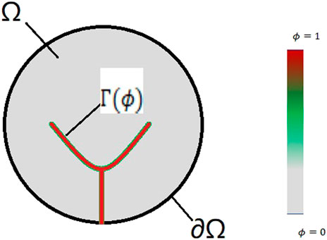
FIGURE 1. Fissures described with a phase-field model.

From formula (2), we can express the total crack surface energy in the elastic body with the following equation

$\begin{array}{c}{\int }_{\mathrm{\Gamma }}{G}_{\mathrm{c}}\mathrm{d}\mathrm{\Gamma }\approx {\int }_{\mathrm{\Omega }}{G}_{\mathrm{c}}\left[\frac{{\left(\varphi -1\right)}^2}{2l_0}+\frac{l_0}{2}|\nabla \varphi {|}^2\right]\mathrm{d}\mathrm{\Omega }\end{array}(3)$

2.2 Elastic strain energy decomposition

According to the above fracture variational criteria, the crack surface energy and elastic strain energy are tied closely. If the elastic strain energy is not decomposed, the pseudo bifurcation of the crack will occur. To solve this problem, this paper decomposes the elastic strain energy in tension and compression based on the method proposed by C. Miehe et al. [32], so that the tensile part of the elastic strain energy drives the evolution of the phase field. To this end, the strain tensor is first spectral decomposed [33]:

${\mathit{\epsilon }}_{\pm }={\displaystyle \sum }_{i=1}^d{⟨{\mathit{\epsilon }}^i⟩}_{\pm }{\mathit{n}}^i\otimes {\mathit{n}}^i(4)$

In the formula, ${\mathit{\epsilon }}_{+}$ and ${\mathit{\epsilon }}_{-}$ are tensile strain tensors and compression strain tensors respectively. ${\mathit{\epsilon }}^i$ and ${\mathit{n}}^i$ are the main strain values and their corresponding directions. $d$ is an independent parameter, namely the spatial dimension. When d = 2, this is a two-dimensional problem. When d = 3, this is a three-dimensional problem. Macaulay brackets in the formula are defined as: < • >+ = (• + | • |)/2,< • >−= (•− | •|)/2.

The strain after spectral decomposition can decompose the elastic strain energy density:

${\psi }_{\mathrm{e}}^{\pm }\left(\mathit{\epsilon }\right)=\frac{\lambda }{2}⟨\mathrm{t}\mathrm{r}\left(\mathit{\epsilon }\right){⟩}_{\pm }^2+\mu \mathrm{t}\mathrm{r}\left({\mathit{\epsilon }}_{\pm }^2\right)(5)$

Here $\mathrm{\lambda }$ and $\mathrm{\mu }$ is the Lame constant, tr (•) represents the trace of the matrix. In the process of material failure, the stiffness will also decrease. At this time, the material stiffness weakening is related to the phase field variable. If we assume that only the tensile strain energy density in the elastic body receives the weakening of the phase field variable, the elastic strain energy at this time is

${\psi }_{\mathrm{e}}\left(\mathit{\epsilon }\right)=\left[{\left(1-\varphi \right)}^2+\mathit{\kappa }\right]{\psi }_{\mathrm{e}}^{+}\left(\mathit{\epsilon }\right)+{\psi }_{\mathrm{e}}^{-}\left(\mathit{\epsilon }\right)(6)$

Where: $\mathit{\kappa }$ is a parameter model parameter, 0 ≤ κ<< 1. Avoid generating numerical singularity when $\mathrm{\varphi }$ = 1.

2.3 Characterization of Drucker-Prager fracture surface

According to Navidtehrani [5–7] Drucker-Prager fracture criterion applicable to brittle or quasi-brittle materials, such as rock or concrete, is shown as follows

$\sqrt{J_2\left(\sigma \right)}=A+B{I}_1\left(\sigma \right)(7)$

$I_1$ and $J_2$ are the first tensor and the second partial derivative of the invariant, respectively.

A is the equation about uniaxial tension (${\sigma }_t)$. B is the equation about uniaxial compression (${\sigma }_c)$. The specific form is as follows

$A=\frac{2}{\sqrt{3}}\left(\frac{{\sigma }_c{\sigma }_t}{{\sigma }_c+{\sigma }_t}\right);B=\frac{1}{\sqrt{3}}\left(\frac{{\sigma }_t-{\sigma }_c}{{\sigma }_c+{\sigma }_t}\right)(8)$

For quasi-brittle materials, the mechanical properties within the Drucker – Prager failure range can still be regarded as linear elastic. Only when the stress reaches the failure surface, the linear elastic behavior will be transformed into non-linear action. At the same time, the failure of the material will lead to the weakening of the tensile strength and compressive strength. We can get the relationship between the material strength and the phase field damage by using the degradation function $g\left(\varphi \right)$ in the numerical calculation:

$\begin{array}{c}A\left(\varphi \right)=\frac{2}{\sqrt{3}}\left(\frac{g\left(\varphi \right){\sigma }_{c}g\left(\varphi \right){\sigma }_t}{g\left(\varphi \right){\sigma }_c+g\left(\varphi \right){\sigma }_t}\right)=g\left(\varphi \right)\frac{2}{\sqrt{3}}\left(\frac{{\sigma }_c{\sigma }_t}{{\sigma }_c+{\sigma }_t}\right)=g\left(\varphi \right)A\left(\varphi =0\right)\\ B\left(\varphi \right)=\frac{1}{\sqrt{3}}\left(\frac{g\left(\varphi \right){\sigma }_t-g\left(\varphi \right){\sigma }_c}{g\left(\varphi \right){\sigma }_c+g\left(\varphi \right){\sigma }_t}\right)=\frac{1}{\sqrt{3}}\left(\frac{{\sigma }_t-{\sigma }_c}{{\sigma }_c+{\sigma }_t}\right)=B\left(\varphi =0\right)\end{array}(9)$

The phase field parameter (𝜙 = 0) represents the integrity of the material. (𝜙 = 1) represents the complete destruction of the material. At this time, the Drucker – Prager parameters are as follows

$A\left(\varphi =1\right)=0;B\left(\varphi =1\right)=B\left(\varphi =0\right)(10)$

Governing equations of phase field fracture model.

Under the condition of considering kinetic energy T at the same time, according to the crack surface energy expressed in Eq.3 and the elastic strain energy density expressed in Eq. 6, the following formula can be obtained:

$T\left(\dot{\mathit{u}}\right)={\int }_{\mathrm{\Omega }}\frac{1}{2}\rho \dot{\mathit{u}}\cdot \dot{\mathit{u}}\mathrm{d}V(11)$

In the formula: ν is the material density. Thus, the expression of Lagrange function can be written:

$L=T-\mathrm{\Pi }={{\displaystyle \int }}_{\mathrm{\Omega }}\frac{1}{2}\rho \dot{\mathit{u}}\cdot \dot{\mathit{u}}\mathrm{d}V-{\int }_{\mathrm{\Omega }}\left\{\left[{\left(1-\varphi \right)}^2+\mathit{\kappa }\right]{\psi }_{\mathrm{e}}^{+}\left(\mathit{\epsilon }\right)+{\psi }_{\mathrm{e}}^{-}\left(\mathit{\epsilon }\right)\right\}\mathrm{d}V-{\int }_{\mathrm{\Omega }}{G}_{\mathrm{c}}\left[\frac{{\varphi }^2}{2l_0}+\frac{l_0}{2}|\nabla \varphi {|}^2\right]\mathrm{d}V(12)$

According to Hamilton’s principle and ignoring the physical force, the Lagrangian function L takes the variation of {$\dot{\mathrm{u}}$, $\mathrm{\varphi }$}, and the control equation of the phase field fracture model can be obtained:

$\left.\mathrm{Div}\left[\mathit{\sigma }\right]=\rho \ddot{\mathit{u}}\left(\frac{G_{\mathrm{c}}}{l_0}+2{\psi }_{\mathrm{e}}^{+}\right)\varphi -G_{\mathrm{c}}{l}_0\Delta \varphi =2{\psi }_{\mathrm{e}}^{+}\right\}(13)$

In the formula: $\mathrm{\sigma }$ is Cauchy stress tensor. We can obtain the stress from the partial derivative of the elastic strain energy corresponding to the strain

$\begin{array}{c}\mathit{\sigma }=\left[{\left(1-\varphi \right)}^2+\kappa \right]{\partial }_{\epsilon }{\psi }_e^{+}\left(\mathit{\epsilon }\right)+{\partial }_{\epsilon }{\psi }_e^{-}\left(\mathit{\epsilon }\right)=\\ \left[{\left(1-\varphi \right)}^2+\kappa \right]\left(\lambda ⟨tr\left(\mathit{\epsilon }\right){⟩}_{+}\mathit{I}+2\mu {\mathit{\epsilon }}_{+}\right)+\lambda ⟨tr\left(\mathit{\epsilon }\right){⟩}_{-}\mathit{I}+2\mu {\mathit{\epsilon }}_{-}\end{array}(14)$

Where: $I$ is the second order unit tensor. The control Eq. 13 is a set of partial differential equations composed of the dynamic balance equation and the phase field evolution equation. In order to make the control equation equal to the aforementioned variational method, the irreversible condition should be added, that is, when the elastomer is under pressure or unloading, the crack healing should be prevented. The simplest and most effective way to deal with the irreversibility of variables is to introduce historical state variables:

$\mathcal{H}\left(\mathit{x},t\right)=\underset{s\in \left[0,t\right]}{\mathit{max}}{\psi }_e^{+}\left[\mathit{\epsilon }\left(\mathit{x},s\right)\right](15)$

The state variable H represents the maximum tensile elastic strain energy. The maximum value of the $\mathcal{H}$ variable from loading to the current time is also related to the relative position and time, that is, $\mathcal{H}\left(x,t\right)$. The irreversibility condition can be satisfied by replacing the value of ∈ ${\psi }_e^{+}$ in Eq. 13 with $\mathcal{H}\left(x,t\right)$ in the control equation. It is also because of the previous irreversible and only increase monotonically. Because of the irreversibility of the state variable $\mathcal{H}$, $\varphi$ also has the same irreversibility and will only increase monotonically. At this time, the control equation should be rewritten as:

$\left.\mathrm{Div}\left[\mathit{\sigma }\right]+\mathit{b}=\rho \ddot{\mathit{u}}\left(\frac{G_{\mathrm{c}}}{l_0}+2\mathcal{H}\right)\varphi -G_{\mathrm{c}}{l}_0\Delta \varphi =2\mathcal{H}\right\}(16)$

Where: $\mathit{b}$ is the body force. The phase field fracture model can describe any behavior of the fracture only by a set of partial differential equations. The separated fracture is equivalent to the fracture field coupled with the displacement field, and no additional tracking of the geometric shape of the tracking crack is required. Therefore, any propagation path of the fracture can be calculated.

2.4 Principle of virtual work. Balance of forces

Now, we will use the principle of virtual work to derive the equilibrium equations of the coupled deformation fracture system. Cauchy stress is introduced $\mathrm{\sigma }$, It is related to the strain $\mathrm{\epsilon }$ Work conjugation. In addition, the traction force $\mathrm{T}$ is defined as partial $\partial \mathrm{\Omega }$ on the solid boundary. We introduce scalar stress into the fracture model $\mathrm{\omega }$. This stress $\mathrm{\omega }$ And phase field $\mathrm{\varphi }$ and phase field micro-stress vector $\mathrm{\xi }$, which conjugate with the phase field gradient $\mathrm{\varphi }$. It is assumed that the phase field $\mathrm{\varphi }$ is only driven by the solution of the displacement problem. Therefore, there is no external traction and $\mathrm{\varphi }$ relevant. In the absence of external force, the principle of virtual work is as follows:

${\int }_{\mathrm{\Omega }}\{\mathrm{\sigma }:\mathrm{\delta }\mathrm{\epsilon }+\mathrm{\omega }\mathrm{\delta }\mathrm{\varphi }+\mathrm{\xi }\cdot \mathrm{\delta }\nabla \mathrm{\varphi }\}\mathrm{d}\mathrm{V}={\int }_{\partial \mathrm{\Omega }}\left(\mathrm{T}\cdot \mathrm{\delta }\mathrm{u}\right)\mathrm{d}\mathrm{S}(17)$

Among δ Represents a virtual quantity. This equation must be applicable to any field Ω and any kinematically permissible change of virtual quantity. Therefore, by applying the Gauss divergence theorem, the local force balance is given by the following formula:

$\begin{array}{c}\nabla \cdot \sigma =0\\ \nabla \cdot \xi -\omega =0\end{array}\mathrm{i}\mathrm{n}\partial \mathrm{\Omega }(18)$

boundary conditions:

$\begin{array}{c}\sigma \cdot \mathbf{n}=\mathbf{T}\\ \xi \cdot \mathbf{n}=0\end{array}\mathrm{o}\mathrm{n}\partial \mathrm{\Omega }(19)$

2.5 Constitutive theory

Based on the phase field crack modeling and theoretical framework, we first discuss the relationship between the change of phase field variables around the crack and the length scale by modifying the degradation function. It is feasible to modify the degradation function under our phase-field model to affect the peak stress of the phase-field model. The following is our equilibrium equation, free energy and related constitutive equation. The balance equation is as follows:

${\sigma }_{ji,j}+b_i=0\mathrm{i}\mathrm{n}V\mathrm{a}\mathrm{n}\mathrm{d}{t}_i={\sigma }_{ji}{n}_j\mathrm{o}\mathrm{n}S(20)$

$\mathrm{V}$ is the volume of the object, $\mathrm{S}$ is its boundary surface, ${\mathrm{n}}_{\mathrm{i}}$ is the unit component (perpendicular to the surface), ${\mathrm{b}}_{\mathrm{i}}$ is the physical strength per unit volume, ${\mathrm{t}}_{\mathrm{i}}$ is the traction vector, ${\mathrm{\sigma }}_{\mathrm{j}\mathrm{i}}$ is the component of Cauchy stress tensor. Assuming small deformation and deformation gradient, make infinitesimal strain tensor ${\mathrm{\epsilon }}_{\mathrm{i}\mathrm{j}}$ can be determined by the deformation gradient of the displacement vector ${\mathrm{u}}_{\mathrm{i}}$ is expressed as,

${\epsilon }_{ij}=\frac{1}{2}\left(u_{i,j}+u_{j,i}\right)(21)$

Phase field parameters usually introduced by phase field method $\mathrm{\varphi }$ .It is used to describe the degradation of materials, and is generally set $\mathrm{\varphi }$ When the boundary changes from 1 to 0, 1 indicates that the material is intact without cracks $\mathrm{\varphi }$ = 0 indicates that the material has been completely destroyed. According to Gurtin’s [34] research, the micro-forces cited at the same time are: a group of micro-forces on the outer surface λ and body micro-force γ, the micro force on the inner surface is $\mathrm{\pi }$ and ${\mathrm{\xi }}_{\mathrm{i}}$, The following is the point direction balance equation of these micro forces:

${\xi }_{i,i}+\gamma +\pi =0\mathrm{i}\mathrm{n}V\mathrm{a}\mathrm{n}\mathrm{d}{\xi }_i{n}_i=\lambda \mathrm{o}\mathrm{n}S(22)$

It can be seen from the second law of thermodynamics in isothermal form that for the system, the sum of the work done by mechanical traction and body force and the work done by external surface and body force is greater than or equal to Helmholtz free energy ψ Total change of. The integral form of the second law is

${\int }_V\dot{\psi }dV\le {\int }_V\left(b_1{\dot{u}}_i+\gamma \dot{\varphi }\right)dV+{\int }_S\left(t_i{\dot{u}}_i+\lambda \dot{\varphi }\right)dS(23)$

Assume that for any volume ψ depends on ${\dot{\mathrm{\epsilon }}}_{\mathrm{i}\mathrm{j}}$, $\mathrm{\varphi }$, and $\dot{\mathrm{\varphi }}$. Under the condition of applying divergence theory, we can determine that Eq. 23 is bound to hold.

$\frac{\partial \psi }{\partial {\epsilon }_{ij}}{\dot{\epsilon }}_{ij}+\frac{\partial \psi }{\partial \varphi }\dot{\varphi }+\frac{\partial \psi }{\partial {\varphi }_{,i}}{\dot{\varphi }}_{,i}+\frac{\partial \psi }{\partial \dot{\varphi }}\ddot{\varphi }\le {\sigma }_{ji}{\dot{\epsilon }}_{ij}-\pi \dot{\varphi }+{\xi }_i{\dot{\varphi }}_{,i}(24)$

According to the standard Coleman and Noll procedure [35], if,

${\sigma }_{ji}=\frac{\partial \psi }{\partial {\epsilon }_{ij}},{\xi }_i=\frac{\partial \psi }{\partial {\varphi }_{,i}},\mathrm{a}\mathrm{n}\mathrm{d}\frac{\partial \psi }{\partial \varphi }=0(25)$

The remaining items lead to unequal reduced dissipation,

$\left(\pi +\frac{\partial \psi }{\partial \varphi }\right)\dot{\varphi }\le 0.(26)$

The attenuation of this dissipative inequality always satisfies the following conditions

$\pi =-\frac{\partial \psi }{\partial \varphi }-\beta \left(\varphi \dot{\varphi },\varphi ,i,{\epsilon }_{ij}\right)\dot{\varphi }(27)$

In the fracture phase field method of brittle materials similar to rock, the value of the $\beta$ is zero.

The following formula introduces a form of Helmholtz free energy to apply the frame to brittle fracture

$\psi =\left[g\left(\varphi \right){\psi }_e^{+}+{\psi }_e^{-}\right]+G_c\left[\frac{3}{8{\mathcal{l}}_0}\left(1-\varphi \right)+\frac{3}{8}{\mathcal{l}}_0{\varphi }_{,i}{\varphi }_{,i}\right](28)$

Among ${\mathrm{\psi }}_{\mathrm{e}}^{+}$ represents the effect of tensile stress on elasticity, ${\mathrm{\psi }}_{\mathrm{e}}^{-}$ represents the effect of compression on elastic strain energy. The study of strain energy decomposition by Borden et al is very profound. For the numerical simulation of brittle fracture, we usually introduce the physical quantity representing the tensile or compressive strength of the material within the elastic limit, namely the elastic modulus E, into the linear elastic isotropic material, as well as the elastic constant Poisson’s ratio ν reflecting the transverse deformation of the material. For our phase-field simulation, we also need to introduce physical quantities such as the effective fracture surface energy ${\mathrm{G}}_{\mathrm{c}}$ per unit area, and the length scale parameter ${\mathcal{l}}_0$. For phase-field fracture simulation, we have mentioned that the variation range of phase-field parameters is between 0 and 1, and the length scale affects the influence range of phase-field parameters.

Rooted in the variational principle of linear elastic fracture energy proposed by Francfort and Marigo [30], and referring to the elliptic regularization method of Mumford-Shah functional in computer image segmentation, it is called AT2 model [36–42], and its manifestation in the phase-field fracture model is ${\left(1-\varphi \right)}^2$. With the failure of the material, the physical properties of the material itself will also change. At this time, we need to use the degradation function, namely $\mathrm{g}$, to determine the weakening of the physical properties of the material. Obviously, our degradation function is related to the phase field parameters. Just as the phase field parameters $\varphi$ only change from 0 to 1, so is our degradation function $g$. When the material is completely destroyed, the degradation function $\mathrm{g}\left(\mathrm{\varphi }\right)$ = 0, we can easily realize the weakening of the elastic property by multiplying it by the elastic energy. The following is the function of the degradation function and the elastic energy equation:

$g\left(\varphi \right)={\left(1-\varphi \right)}^2(29)$

According to our degradation function, it is easy to obtain the peak stress:

${\sigma }_c=\sqrt{\frac{3G_{c}E}{8{\mathcal{l}}_0}}(30)$

The final governing equation is as follows:

$\left({\varphi }^2\frac{\partial {\psi }_e^{+}}{\partial {\epsilon }_{ij}}+\frac{\partial {\psi }_e^{-}}{\partial {\epsilon }_{ij}}\right)+b_i=\beta \dot{\varphi }\mathrm{i}\mathrm{n}\mathrm{V}\left({\varphi }^2\frac{\partial {\psi }_e^{+}}{\partial {\epsilon }_{ij}}+\frac{\partial {\psi }_e^{-}}{\partial {\epsilon }_{ij}}\right)n_j=t_i\mathrm{o}\mathrm{n}\mathrm{S}(31)$

And

$\frac{3}{8}{G}_c{\mathcal{l}}_0{\varphi }_{,ii}+\frac{3G_c}{8{\mathcal{l}}_0}-2\varphi {\psi }_e^{+}+\gamma =0inV,\frac{3}{8}{G}_c{\mathcal{l}}_0{\varphi }_{,i}{n}_i=\lambda onS(32)$

3 The degradation function

For the sake of completeness, we introduce the degradation function proposed by Lo et al [18, 20]. In this section. Eq. 30 shows that the peak stress is not only related to the properties of the material itself, such as material strength ${\sigma }_c$. Breaking energy ${\mathrm{G}}_{\mathrm{c}}$ is related to Young’s modulus E, and also to the phase field length scale ${\mathcal{l}}_0$. Because of our need for numerical simulation of large-scale rock phase field fracture, the phase field length scale is usually a very small physical quantity. This has brought a great burden to our actual calculation. We can easily associate whether we can decouple the peak stress and the phase field length scale if we adopt a new degradation function to ensure more efficient calculation results. Therefore, we adopt the following degradation function:

$g\left(\varphi \right)=\mathrm{s}\left[1-{\left(\frac{s-1}{s}\right)}^{{\varphi }^2}\right](33)$

As shown in Figure 2, the function curve under different s values. The characteristic of this degradation function is that a parameter s is introduced to control the specific peak stress through different values of s. We can easily calculate the peak stress of different s values by the following formula.

${\sigma }_c^{*}=\frac{\sqrt{\frac{3G_{c}E}{8{\mathcal{l}}_0}}}{\sqrt{\left(s-1\right)\ln \left(\frac{s}{s-1}\right)}}(34)$

FIGURE 2

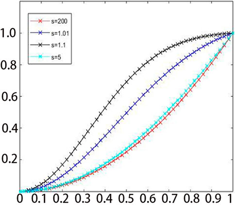
FIGURE 2. The curvature of the degradation function is controlled by the parameter s, corresponding to different change rates. For large s values, the change of degradation function is similar to that of traditional AT2 model.

we separate the phase field length scale ${\mathcal{l}}_0$ and the physical length scale ${\mathcal{l}}_{\mathrm{p}}$. In the traditional phase field simulation, ${{\mathcal{l}}_0=\mathcal{l}}_{\mathrm{p}}$, and we choose different s values, the corresponding phase field length scale ${\mathcal{l}}_0$ and the physical length scale lp ratio are also different, and the corresponding physical length scale ${\mathcal{l}}_{\mathrm{p}}$ formula is

${\mathcal{l}}_{\mathrm{p}}=\left(s-1\right)\ln \left(\frac{s}{s-1}\right){\mathcal{l}}_0(35)$

At this time, the ratio of peak stress is also different. We use the new peak stress symbol ${\sigma }_c^{*}$ to distinguish,

${\sigma }_c^{*}=\sqrt{\frac{3G_{c}E}{8{\mathcal{l}}_p}.}(36)$

For the value of s, we can find that when s ≈ 1.0148, ${\mathcal{l}}_0$ increase by 16 times with the peak stress unchanged. This has increased by an order of magnitude, and if we want to increase ${\mathcal{l}}_0$ 100 times while maintaining the same peak stress, when s ≈ 1.00155. With different values of s, we can easily simulate a larger scale model, which has many advantages for the phase field modeling of our large-scale rock mass model.

4 Numerical examples

4.1 Tension square plate with unilateral crack

Consider the tension square plate containing initial cracks as shown in Figure 3Awith a side length of 50 mm, which is divided into 46118 quadrilateral elements as shown in Figure 3B, and locally densified at the predicted crack growth path, where the grid size is about 0.1 mm. Let the problem be a plane strain problem, with an elastic modulus of 250 kN/mm², a Poisson’s ratio of 0.2, and a fracture toughness of Gc = 2.5 × 10−³ kN/mm². Using displacement loading method, t = 1s, ΔU = 0.15 mm until complete failure. During the calculation, l₀ = 0.2 mm is taken. First, the geometric discontinuity method is used to preset the initial crack, that is, the upper and lower elements are geometrically separated at the crack. The calculated crack growth process is shown in Figure 3.

FIGURE 3

FIGURE 3. (A) Square plate under tension/m. (B) Meshing diagram (Tight zone dimensions = 0.2, other = 1) (C) Crack propagation path (S = 5). (D) Crack propagation path (S = 200). (E) Crack propagation path (traditional degradation).

Based on the numerical simulation results presented in Figures 3, 4, it can be observed that the model employing our proposed phase-field fracture method generates a crack propagation path that is more complex and closely resembles a rock fracture section during the simulation of the tensile square plate. Conversely, the crack growth path generated by the traditional degradation function appears more linear. These findings indicate that our proposed phase-field fracture model possesses distinctive characteristics in accurately capturing crack propagation under complex stress-displacement boundary conditions, which enables it to fit large-scale rock models while maintaining crack tracking precision. Consequently, further numerical simulations will be conducted to comprehensively investigate, analyze and compare the performance of our proposed model.

FIGURE 4

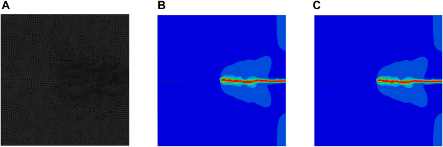
FIGURE 4. (A) Meshing diagram = 0.4. (B) Crack propagation path (S = 1.107). (C) Crack propagation path (S = 1.01).

4.2 Shear square plate with unilateral crack

The same material parameters as in Example 4.1 are used to study the crack growth process of square plates under shear. The calculation model is shown in Figure 5A, and the vertical displacement on all boundaries is constrained to zero. The displacement loading method is adopted, and the displacement increment of each loading step is Δ U = 2.5mm, the non-uniform grid is adopted, and the grid is densified at the position where the crack growth is expected. The minimum grid size is about 0.2 mm. The grid model is shown in Figure 5B.

FIGURE 5

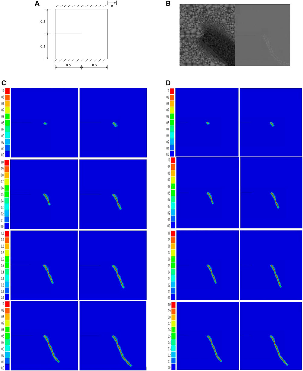
FIGURE 5. (A) Sheared square plates. (B) Meshing diagram (Tight zone dimensions = 0.2, other = 1) (C) Crack propagation path (S = 200). (D) Crack propagation path (traditional degradation).

In the experiment involving a shear square plate with a unilateral crack, numerical simulations were conducted by varying the S value (S = 200), and the results obtained are shown in Figures 5D, E. Comparison of these results with those obtained by the traditional degradation function, such as Figure 5C, reveals that the tracked crack propagation path remains the same. This observation is consistent with our theoretical calculations of the relationship between S value and peak stress.

For the following research, we plan to investigate the effect of varying the S value on the physical and phase field scales. Specifically, we will choose values of S = 1.01 and 1.1 to expand the physical scale and the multiple of the phase field scale. The choice of S = 1.01 will result in a phase field scale that is 16 times the physical scale, while S = 1.107 will yield a phase field scale that is 4 times the physical scale. The model cell mesh size will be set to 0.4 mm. Through this verification process, we aim to demonstrate that our phase-field model has lower demands for mesh accuracy than the traditional phase-field model.

Based on the results presented in Figure 6, it can be observed that a gradual decrease of parameter S leads to an increase in the proportion of phase field length to physical length. This results in the phase field length being several times or even ten times greater than the physical length. As the proportional relationship between the mesh density and phase field length is a key factor affecting fracture tracking accuracy in the phase-field method, it is possible to reduce the mesh density without compromising the accuracy of crack tracking, as long as the proportion of mesh density and phase field length is maintained. This outcome is highly valuable for large-scale rock numerical simulations, as it results in significant computational resource savings and enhances the efficacy of the phase-field method for such applications.

FIGURE 6

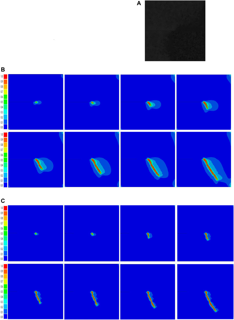
FIGURE 6. (A) Meshing diagram (Tight zone dimensions = 0.4). (B) Crack propagation path (S = 1.107). (C) Crack propagation path (S = 1.01).

4.3 Direct shear test of cracked plates

Next, direct shear tests are simulated to evaluate the degradation function changes in the test configuration. The geometry and boundary conditions of the model are shown in Figure 7A. Apply a lateral displacement on the top edge, which is equal to 0.15 mm. The boundary conditions are vertical constraints at the top and fixed constraints at the bottom. Modulus of elasticity E = 25 GPa and Poisson’s ratio ν = 0.2, fracture parameters are given by Gc = 0.15 kJ/m² and l = 0.2 mm. In order to save computing resources, the predicted crack propagation area is encrypted, and the cell size of the encrypted part is at least half of the phase field scale, so as to save computer resources without affecting the computing accuracy.

FIGURE 7

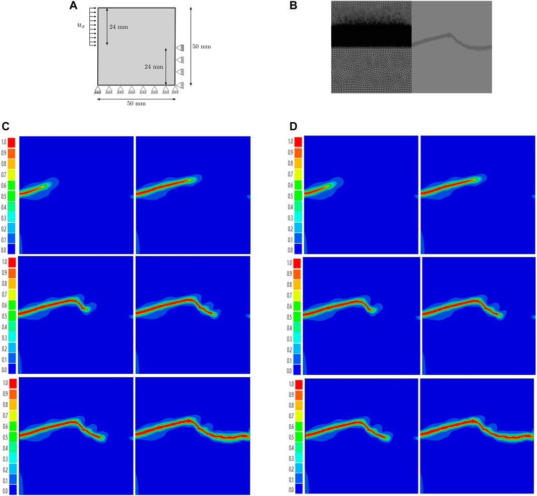
FIGURE 7. (A) Direct shear test (DST). (B) Meshing diagram (Tight zone dimensions = 0.1, other = 1) and the calculated crack growth process. (C) Crack propagation path (S = 200). (D) Crack propagation path (traditional degradation).

The crack initiation and propagation mode observed in the simulation is in line with the rock shear fracture experiment, where the crack initiates from the edge and progresses towards the center. The simulation results presented in the figure above compare the crack growth path obtained using the specific degradation function with S = 200 and the traditional degradation function. The result display that the crack propagation paths traced by the traditional degradation function are similar when S = 200.

As the value of S approaches 1, the phase field characteristic length and the physical characteristic length become decoupled, resulting in a change in the quantitative relationship between the phase field length and physical scale. This leads to a significant increase in the phase field scale, which can become several times or even dozens of times larger than the physical scale. For instance, when S = 1.107, the phase field scale is observed to be four times larger than the physical scale. To accurately track the crack propagation path using the phase field method, a smaller mesh size than the phase field scale is required. Therefore, with the increase in phase field scale, excessively dense grids can be discarded. By maintaining the proportion between the phase field scale and mesh size, a mesh size of 0.4 mm can be set to achieve equally accurate crack propagation path tracking.

As shown in Figure 8, when using a smaller S value, increase the cell size of the model and use a 0.04 mm mesh size. At this time, very accurate crack tracking curve of rock direct shear test can still be obtained. It is verified that this phase field model can more effectively simulate large-scale rock fracture.

FIGURE 8

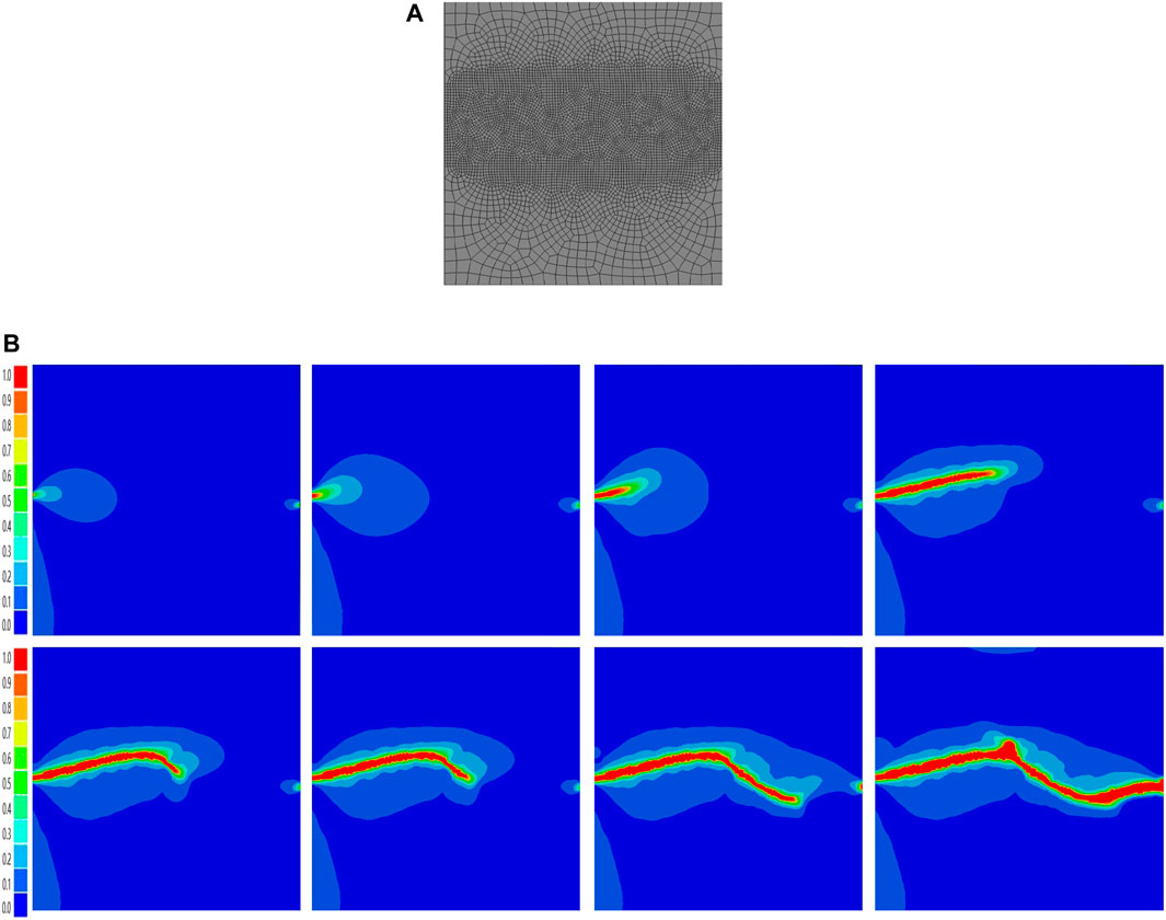
FIGURE 8. (A) Meshing diagram (Tight zone dimensions = 0.5, other = 2). (B) Crack propagation path (S = 1.107).

4.4 Notched plate with eccentric holes

In this case, we model the rock plate with holes, as shown in the figure. This is an eccentric plate with three holes with a length of 120 mm and a width of 70 mm. The size and distribution of the holes are indicated in the Figure 9 below. The boundary condition is that the bottom is fixed vertically and horizontally, and 0.15 mm vertical displacement is applied to the top. The material property parameter in this simulation is Young’s modulus E = 25 GPa, Poisson’s ratio ν = 0.20, Phase field scale ${\mathcal{l}}_0$ = 0.25 mm and energy release rate Gc = 0.15 kJ/m². At the same time, we compare the different degradation functions affected by multiple S and the cracks tracked by the traditional degradation functions, and use the same division ratio for the element, that is, the mesh size is equal to 0.1 mm. See the figure below for the specific numerical simulation results.

FIGURE 9

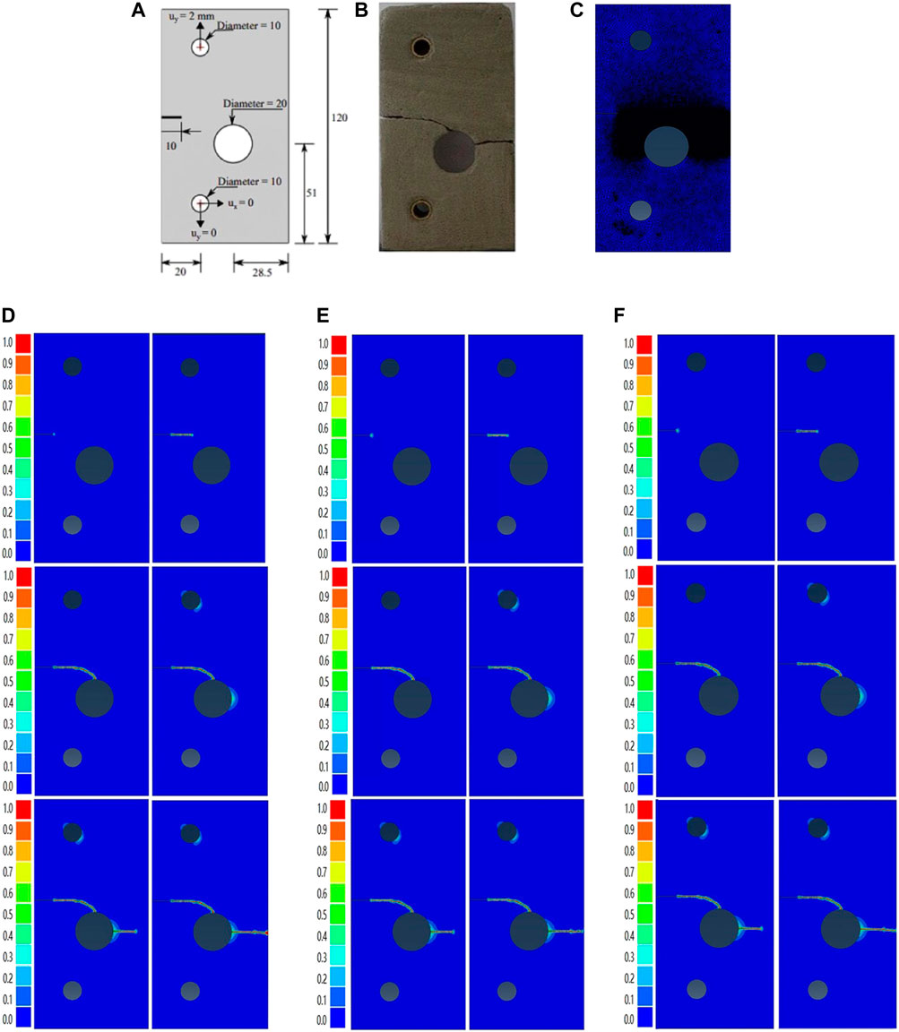
FIGURE 9. (A) Boundary conditions and geometric parameters (B) actual experimental results (C) Meshing diagram (Tight zone dimensions=0.1, other=1) (D) Crack propogation path (S=5) (E) Crack propogation path (S=200) (F) Crack propogation path (traditional degradation).

In notched rock slabs with eccentric holes, obtaining accurate crack information is crucial, as multiple factors affect the crack propagation process. In this simulation, we employed the traditional phase field model of Drucker-Prager fracture criterion and the traditional degradation function for numerical simulation, and the simulation results are depicted in Figures 9, 10. Comparing Figures 10 B, C, if we exaggerate the phase field length while maintaining the original set mesh density, our crack path will shift. At this time, we can alleviate this problem by keeping the proportion of the enlarged grid density and the phase field length the same, that is, the grid density is less than half of the phase field scale. Even so, the mesh density after densification is still much smaller than the initially given mesh density, which is more conducive to obtaining the correct crack path and more efficient numerical simulation. However, we can overcome this issue by densifying the mesh. Through multiple sets of experimental simulations, we determined that a phase field scale with a grid density less than half can accurately track the crack propagation path.

FIGURE 10

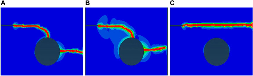
FIGURE 10. (A) Crack propagation path S = 1.107 (element size 0.4). (B) Crack propagation path S = 1.107 (element size 0.4). (C) Crack propagation path S = 1.107 (element size 1.0).

5 Conclusion

This study effectively accelerates the fracture phase field modeling for compressive failure of rocks materials. By splitting the strain energy using the approach introduced by [18, 20], the asymmetric tension-compression behaviors in rock fracture processes can be characterized. To decouple the phase-field length with the physical length scale, the degradation function proposed by [18, 20] were adopted and thus the mesh density is reduced for the structures much larger than the physical process zone. In the future, we will extend the present approach to the applications of hydraulic fracturing in quasi-brittle materials [43]. In addition, the combination of isogeometric analysis will be considered to solve high-order problems [44].

Data availability statement

The original contributions presented in the study are included in the article/supplementary material, further inquiries can be directed to the corresponding author.

Author contributions

BL: optical experiment, ZL and LY: guidance and revision.

Funding

The authors are grateful for the support of National Natural Science Foundation of China (Nos. 52174213, 51574174).

Conflict of interest

The authors declare that the research was conducted in the absence of any commercial or financial relationships that could be construed as a potential conflict of interest.

Publisher’s note

All claims expressed in this article are solely those of the authors and do not necessarily represent those of their affiliated organizations, or those of the publisher, the editors and the reviewers. Any product that may be evaluated in this article, or claim that may be made by its manufacturer, is not guaranteed or endorsed by the publisher.

References

1. Jaeger JC, Cook NJ. Fundamental of rock mechanics (1979). doi:10.1016/j.mineng.2009.02.015

CrossRef Full Text | Google Scholar

2. León Baldelli AA, Maurini C. Numerical bifurcation and stability analysis of variational gradient-damage models for phase-field fracture. J Mech Phys Sol (2021) 152:104424. doi:10.1016/j.jmps.2021.104424

CrossRef Full Text | Google Scholar

3. Zhuang XY, Zhou SW, Sheng M, Li GS. On the hydraulic fracturing in naturally-layered porous media using the phase field method. ENGINEERING GEOLOGY (2020) 266:105306. doi:10.1016/j.enggeo.2019.105306

CrossRef Full Text | Google Scholar

4. Zhang Q, Wang D, Zeng F, Guo Z, Wei N. Pressure transient behaviors of vertical fractured wells with asymmetric fracture patterns. JOURNAL ENERGY RESOURCES TECHNOLOGY-TRANSACTIONS ASME (2020) 142(4). doi:10.1115/1.4045226

CrossRef Full Text | Google Scholar

5. Navidtehrani Y, Betegon C, Martinez-Paneda E. A unified abaqus implementation of the phase field fracture method using only a user material subroutine. MATERIALS (2021) 14(8):1913. doi:10.3390/ma14081913

PubMed Abstract | CrossRef Full Text | Google Scholar

6. Navidtehrani Y, Betegon C, Martinez-Paneda E. A general framework for decomposing the phase field fracture driving force, particularised to a Drucker-Prager failure surface. THEORETICAL APPLIED FRACTURE MECHANICS (2022) 121. doi:10.1016/j.tafmec.2022.103555

CrossRef Full Text | Google Scholar

7. Navidtehrani Y, Betegon C, Zimmerman RW, Martinez-Paneda E. Griffith-based analysis of crack initiation location in a Brazilian test. INTERNATIONAL JOURNAL ROCK MECHANICS MINING SCIENCES (2022) 159:105227. doi:10.1016/j.ijrmms.2022.105227

CrossRef Full Text | Google Scholar

8. Cundall PA. A computer model for simulating progressive large-scale movements in blocky rock systems. In: Proceedings of the Symposium of the International Society for Rock Mechanics, Society for Rock Mechanics (ISRM); 1971; France, Paris (1971). p. 11–8.

Google Scholar

9. Li H, Huang Y, Yang Z, Yu K, Li QM. 3D meso-scale fracture modelling of concrete with random aggregates using a phase-field regularized cohesive zone model. Int J Sol Structures (2022) 256:111960. doi:10.1016/j.ijsolstr.2022.111960

CrossRef Full Text | Google Scholar

10. Carlsson J, Isaksson P. A statistical geometry approach to length scales in phase field modelling of fracture and strength of porous microstructures. Int J Sol Structures (2020) 200-201:83–93. doi:10.1016/j.ijsolstr.2020.05.003

CrossRef Full Text | Google Scholar

11. Borden MJ, Hughes TJR, Landis CM, Anvari A, Lee IJ. Corrigendum to “A phase-field formulation for fracture in ductile materials: Finite deformation balance law derivation, plastic degradation, and stress triaxiality effects. Comp Methods Appl Mech Eng (2017) 324:712–3. doi:10.1016/j.cma.2017.06.023

CrossRef Full Text | Google Scholar

12. Jiang D, Kyriakides S, Landis CM. Propagation of phase transformation fronts in pseudoelastic NiTi tubes under uniaxial tension. Extreme Mech Lett (2017) 15:113–21. doi:10.1016/j.eml.2017.06.006

CrossRef Full Text | Google Scholar

13. Jiang D, Kyriakides S, Landis CM, Kazinakis K. Modeling of propagation of phase transformation fronts in NiTi under uniaxial tension. Eur J Mech - A/Solids (2017) 64:131–42. doi:10.1016/j.euromechsol.2017.02.004

CrossRef Full Text | Google Scholar

14. Landis CM, Beyerlein IJ, McMeeking RM. Micromechanical simulation of the failure of fiber reinforced composites. J Mech Phys Sol (2000) 48(3):621–48. doi:10.1016/S0022-5096(99)00051-4

CrossRef Full Text | Google Scholar

15. Landis CM, Huang R, Hutchinson JW. Formation of surface wrinkles and creases in constrained dielectric elastomers subject to electromechanical loading. J Mech Phys Sol (2022) 167:105023. doi:10.1016/j.jmps.2022.105023

CrossRef Full Text | Google Scholar

16. Li W, Landis CM. Nucleation and growth of domains near crack tips in single crystal ferroelectrics. Eng Fracture Mech (2011) 78(7):1505–13. doi:10.1016/j.engfracmech.2011.01.002

CrossRef Full Text | Google Scholar

17. Li W, McMeeking RM, Landis CM. On the crack face boundary conditions in electromechanical fracture and an experimental protocol for determining energy release rates. Eur J Mech - A/Solids (2008) 27(3):285–301. doi:10.1016/j.euromechsol.2007.08.007

CrossRef Full Text | Google Scholar

18. Lo Y-S, Borden MJ, Ravi-Chandar K, Landis CM. A phase-field model for fatigue crack growth. J Mech Phys Sol (2019) 132:103684. doi:10.1016/j.jmps.2019.103684

CrossRef Full Text | Google Scholar

19. Woldman AY, Landis CM. Thermo-electro-mechanical phase-field modeling of paraelectric to ferroelectric transitions. Int J Sol Structures (2019) 178-179:19–35. doi:10.1016/j.ijsolstr.2019.06.012

CrossRef Full Text | Google Scholar

20. Lo Y-S, Hughes TJR, Landis CM. Phase-field fracture modeling for large structures. J Mech Phys Sol (2023) 171:105118. doi:10.1016/j.jmps.2022.105118

CrossRef Full Text | Google Scholar

21. Ai W, Wu B, Martínez-Pañeda E. A coupled phase field formulation for modelling fatigue cracking in lithium-ion battery electrode particles. J Power Sourc (2022) 544:231805. doi:10.1016/j.jpowsour.2022.231805

CrossRef Full Text | Google Scholar

22. Cui C, Ma R, Martínez-Pañeda E. A generalised, multi-phase-field theory for dissolution-driven stress corrosion cracking and hydrogen embrittlement. J Mech Phys Sol (2022) 166:104951. doi:10.1016/j.jmps.2022.104951

CrossRef Full Text | Google Scholar

23. Isfandbod M, Martínez-Pañeda E. A mechanism-based multi-trap phase field model for hydrogen assisted fracture. Int J Plasticity (2021) 144:103044. doi:10.1016/j.ijplas.2021.103044

CrossRef Full Text | Google Scholar

24. Kristensen PK, Niordson CF, Martínez-Pañeda E. A phase field model for elastic-gradient-plastic solids undergoing hydrogen embrittlement. J Mech Phys Sol (2020) 143:104093. doi:10.1016/j.jmps.2020.104093

CrossRef Full Text | Google Scholar

25. Martínez-Pañeda E, Fuentes-Alonso S, Betegón C. Gradient-enhanced statistical analysis of cleavage fracture. Eur J Mech - A/Solids (2019) 77:103785. doi:10.1016/j.euromechsol.2019.05.002

CrossRef Full Text | Google Scholar

26. Navidtehrani Y, Betegón C, Martínez-Pañeda E. A simple and robust Abaqus implementation of the phase field fracture method. Appl Eng Sci (2021) 6:100050. doi:10.1016/j.apples.2021.100050

CrossRef Full Text | Google Scholar

27. Navidtehrani Y, Betegón C, Martínez-Pañeda E. A general framework for decomposing the phase field fracture driving force, particularised to a Drucker–Prager failure surface. Theor Appl Fracture Mech (2022) 121:103555. doi:10.1016/j.tafmec.2022.103555

CrossRef Full Text | Google Scholar

28. Tan W, Martínez-Pañeda E. Phase field fracture predictions of microscopic bridging behaviour of composite materials. Compos Structures (2022) 286:115242. doi:10.1016/j.compstruct.2022.115242

CrossRef Full Text | Google Scholar

29. Espadas-Escalante JJ, Van Dijk NP, Isaksson Pjcs T. A phase-field model for strength and fracture analyses of fiber-reinforced composites. Compos Sci Technol (2019) 174(APR.12):58–67. doi:10.1016/j.compscitech.2018.10.031

CrossRef Full Text | Google Scholar

30. Bourdin B, Francfort GA, Marigo JJ. Numerical experiments in revisited brittle fracture. J Mech Phys Sol (2000) 48(4):797–826. doi:10.1016/S0022-5096(99)00028-9

CrossRef Full Text | Google Scholar

31. Miehe C, Welschinger F, Hofacker M. Thermodynamically consistent phase-field models of fracture: Variational principles and multi-field FE implementations. Int J Numer Methods Eng (2010) 83(10):1273–311. doi:10.1002/nme.2861

CrossRef Full Text | Google Scholar

32. Miehe C, Hofacker M, Welschinger F. A phase field model for rate-independent crack propagation: Robust algorithmic implementation based on operator splits. Comp Methods Appl Mech Eng (2010) 199(45):2765–78. doi:10.1016/j.cma.2010.04.011

CrossRef Full Text | Google Scholar

33. Bernard PE, Moës N, Chevaugeon N. Damage growth modeling using the Thick Level Set (TLS) approach: Efficient discretization for quasi-static loadings. Comp Methods Appl Mech Eng (2012) 233-236:11–27. doi:10.1016/j.cma.2012.02.020

CrossRef Full Text | Google Scholar

34. Gurtin ME. Generalized Ginzburg-Landau and Cahn-Hilliard equations based on a microforce balance. Physica D: Nonlinear Phenomena (1996) 92(3):178–92. doi:10.1016/0167-2789(95)00173-5

CrossRef Full Text | Google Scholar

35. Coleman BD, Noll W. The thermodynamics of elastic materials with heat conduction and viscosity. In: W Noll, editor. The foundations of mechanics and thermodynamics: Selected papers. Berlin, Heidelberg: Springer Berlin Heidelberg (1974). p. 145–56.

CrossRef Full Text | Google Scholar

36. Feng D-C, Wu J-Y. Phase-field regularized cohesive zone model (CZM) and size effect of concrete. ENGINEERING FRACTURE MECHANICS (2018) 197:66–79. doi:10.1016/j.engfracmech.2018.04.038

CrossRef Full Text | Google Scholar

37. Vinh Phu N, Wu J-Y. Modeling dynamic fracture of solids with a phase-field regularized cohesive zone model. COMPUTER METHODS APPLIED MECHANICS ENGINEERING (2018) 340:1000–22. doi:10.1016/j.cma.2018.06.015

CrossRef Full Text | Google Scholar

38. Wu J-Y. A unified phase-field theory for the mechanics of damage and quasi-brittle failure. JOURNAL MECHANICS PHYSICS SOLIDS (2017) 103:72–99. doi:10.1016/j.jmps.2017.03.015

CrossRef Full Text | Google Scholar

39. Wu J-Y. A geometrically regularized gradient-damage model with energetic equivalence. COMPUTER METHODS APPLIED MECHANICS ENGINEERING (2018) 328:612–37. doi:10.1016/j.cma.2017.09.027

CrossRef Full Text | Google Scholar

40. Wu J-Y. Robust numerical implementation of non-standard phase-field damage models for failure in solids. COMPUTER METHODS APPLIED MECHANICS ENGINEERING (2018) 340:767–97. doi:10.1016/j.cma.2018.06.007

CrossRef Full Text | Google Scholar

41. Wu J-Y, Vinh Phu N. A length scale insensitive phase-field damage model for brittle fracture. JOURNAL MECHANICS PHYSICS SOLIDS (2018) 119:20–42. doi:10.1016/j.jmps.2018.06.006

CrossRef Full Text | Google Scholar

42. Wu J-Y, Vinh Phu N, Nguyen CT, Sutula D, Sinaie S, Bordas SPA. Phase-field modeling of fracture. In: SPA Bordas, and DS Balint, editors, 53 (2020). p. 1–183.ADVANCES APPLIED MECHANICS

CrossRef Full Text | Google Scholar

43. Yang J, Lian H, Nguyen VP. Study of mixed mode I/II cohesive zone models of different rank coals. Eng Fracture Mech (2021) 246:107611. doi:10.1016/j.engfracmech.2021.107611

CrossRef Full Text | Google Scholar

44. Chen L, Wang Z, Peng X, Yang J, Wu P, Lian H. Modeling pressurized fracture propagation with the isogeometric BEM. Geomechanics Geophys Geo-Energy Geo-Resources (2021) 7(3):51. doi:10.1007/s40948-021-00248-3

CrossRef Full Text | Google Scholar