Synchronization transitions on connectome graphs with external force

We investigate the synchronization transition of the Shinomoto-Kuramoto model on networks of the fruit-fly and two large human connectomes. This model contains a force term, thus is capable of describing critical behavior in the presence of external excitation. By numerical solution we determine the crackling noise durations with and without thermal noise and show extended non-universal scaling tails characterized by the exponent 2 < τ_t < 2.8, in contrast with the Hopf transition of the Kuramoto model, without the force τ_t = 3.1(1). Comparing the phase and frequency order parameters we find different synchronization transition points and fluctuation peaks as in case of the Kuramoto model, related to a crossover at Widom lines. Using the local order parameter values we also determine the Hurst (phase) and β (frequency) exponents and compare them with recent experimental results obtained by fMRI. We show that these exponents, characterizing the auto-correlations are smaller in the excited system than in the resting state and exhibit module dependence.

1 Introduction

The critical brain hypothesis has been confirmed experimentally many times since the pioneering electrode experiments in [1]. Power law (PL) distributed neuronal avalanches were shown in neuronal recordings (spiking activity and local field potentials, LFPs) of neural cultures in vitro [2–4], LFP signals in vivo [5], field potentials and functional magnetic resonance imaging (fMRI) blood-oxygen-level-dependent (BOLD) signals in vivo [6, 7], voltage imaging in vivo [8], 10–100 and single-unit or multi-unit spiking and calcium-imaging activity in vivo [9–12]. Furthermore, source reconstructed magneto- and electroencephalographic recordings (MEG and EEG), characterizing the dynamics of ongoing cortical activity, have also shown non-universal PL scaling in neuronal long-range temporal correlations [13, 14]. Optical methods, like light-sheet microscopy with GCaMP zebrafish larvae [15] or calcium imaging recordings of dissociated neuronal cultures [16] also show PL scaling.

From a theoretical point of view the hypothesis is also very attractive as critical systems possess optimal computational capabilities as well as provide efficient long range communications, memory and sensitivity [17–28].

Homogeneous critical systems exhibit universal scaling behavior and many experiments claim indeed a mean-field class behavior of the branching process [29, 30] generated by self-organized criticality [31]. However, neural systems are very non-homogeneous, thus it is natural to expect non-universal behavior, known in statistical physics within the field of quenched disordered models [32, 33]. Indeed some experiments [13, 14, 16] show that the measured exponents are not universal, significantly different from the mean-field class ones of the branching process.

Furthermore, external sources can move the system away from criticality [34, 35] or tune it to other classes, like the isotropic percolation [16, 36] or to tricritical points [37]. More complex models than the two-state branching process, can also exhibit hybrid type of phase transitions, like threshold models [38], models with inhibitory nodes [39] or models with oscillatory units [40]. Subsystems can also show different scaling behavior and may be within different distances from criticality [41].

For quenched disordered models it has recently been shown [42, 43], that even for weak time dependence the semi-critical, dynamical scaling, which occurs in an extended control parameter region of criticality, in the so called Griffihts Phases [44] (GP), remains stable. Furthermore, even when the network dimension is high, one does not find the usual mean-field behavior, but in the presence of modules a GP [36, 38, 45–48] or Griffihts effects [49] and a different, sometimes logarithmically slow scaling at the critical point [32].

The big advantage of critical universality is that more realistic models for the brain, like the integrate and fire models [50], can also show the same criticality as simpler ones like in a recent work [51], which derives Hopf bifurcation criticality or in a more experimental study [52] of neural cultures agreement with isotropic percolation avalanche size distributions is obtained. But of course the directed percolation criticality [53, 54], which occurs in branching processes [1] is the main example for the universality principle [55]. Therefore, the study of simpler models, for which numerical analysis can be done are very useful for the brain science [28, 33].

Recently threshold models and Kuramoto type of models have been analyzed on different, available connectome networks and GP behavior was reported [33, 43, 56–59]. This behavior is also called as frustrated synchronization [60–62] and has been analyzed within the framework of a Kuramoto like models, albeit lacking quenched self-frequencies.

From the experimental directions the different behavior in modules of brains of the mouse [41], by phenomenological renormalization-group analysis of the spectrum of electrode spikes, and humans [63], via Hurst and β exponents analysis of fMRI; quasi-critical (off-critical) scaling like behavior has been shown. Here we attempt to model this using the Shinomoto–Kuramoto (SK) model on connectomes of the fruit-fly (FF) and humans. This is an extension of the Kuramoto model [64], which itself does not have an external source, that can describe the resting state critical behavior at the Hopf transition towards a model with a periodic external driving force, thus may be appropriate to characterize criticality with an excitation [40].

2 Models and methods

In this Section we introduce the synchronization model, followed by an overview of different connectome graphs, on which we run the numerical analysis. Finally we discuss the method of local synchronization to dig into the details of the spatio-temporal simulations of these brain systems.

2.1 The Shinomoto–Kuramoto (SK) model

We consider an extension of the Kuramoto model [64] of interacting oscillators sitting at the nodes of a network, whose phases θ_j(t), j = 1, 2, … N evolve according to the following set of dynamical equations

$\begin{array}{ll}\hfill {\dot{\theta }}_j\left(t\right)& ={\omega }_j^0+K\sum _k{W}_{jk}\sin \left[{\theta }_k\left(t\right)-{\theta }_j\left(t\right)\right]\hfill \\ \hfill & +F\sin \left({\theta }_j\left(t\right)\right)+ϵ{\eta }_j\left(t\right).\hfill \end{array}(1)$

Here, ${\omega }_j^0$ is the so-called self-frequency of the jth oscillator, which is drawn from a Gaussian distribution with zero mean and unit variance. The summation is performed over adjacent nodes, coupled by the W_jk matrix. Up to this point we have the classical Kuramoto model [64]. In the Shinomoto extension [65], we have a Gaussian annealed noise term η_j(t), with an amplitude ϵ, and to describe excitation, a site dependent periodic force term, proportional to a coupling F.

Sakaguchi [66] was the first to study the periodically forced Kuramoto model. In numerical simulations, however, he found that the state of forced entrainment was not always attained: macroscopic fractions of the system self-synchronized at a different frequency from that of the drive, indicating that this sub-population had broken away and established its own collective rhythm. Analytically improvements were provided in [67–69] and found a rich phase space of the SK model.

Recently, in [40] the avalanche behavior of the SK equation was investigated, albeit with site independent self-frequencies ${\omega }_j^0=\omega$. The authors explored the phase diagram, besides the forceless Hopf transition a so-called saddle node invariant cycle (SNIC) and a hybrid type of bifurcation were compared. In a very recent publication [48], this numerical analysis has been continued on Erdős–Rényi (ER) and hierarchical modular networks, motivated by brain research. Considering quenched ${\omega }_j^0$-s with bi-modal frequency distributions the authors claim the emergence of Griffiths effects by the broadening of the synchronization transition region.

Here we study the SK model using quenched ${\omega }_j^0$-s with and without annealed noise η_j(t) on real connectomes. In particular we test if the chaoticity, generated by the quenched ${\omega }_j^0$-s generates the same phase transition behavior and avalanches as with the presence of the stochastic noise. We measured the Kuramoto phase order parameter:

$z\left(t\right)=r\left(t\right)\exp i\theta \left(t\right)=1/N\sum _j\exp \left[i{\theta }_j\left(t\right)\right],(2)$

by increasing the sampling time steps δt = 0.01. Here 0 ≤ r(t) ≤ 1 gauges the overall coherence and θ(t) is the average phase. The set of Eq. 1 was solved by the steppers Runge–Kutta-4 (RK4), for the noisy, or by the Bulrisch–Stoer [70, 71] (BS) for the noiseless cases, because in the presence of noise the adaptive BS fails to work. Here and in earlier studies [58] we found that stronger stochastic noise makes the results non-reliable, while application of other steppers slows down the numerical solution. For the noisy cases we also tried the Euler–Maruyama solver [72], which has a stronger mathematical foundation for stochastic differential equations. This had to be restricted to testing purposes only, as this first-order solver is orders of magnitude slower than the RK4 for the same precision.

We integrated the set of equations numerically for 10³–10⁴ independent initial conditions, by different ${\omega }_j^0$-s and sample averages of the phases

$R\left(t\right)=⟨r\left(t\right)⟩(3)$

and of the variance of the frequencies

$\mathrm{\Omega }(t)=⟨\frac{1}{N}\sum _{j=1}^N{(\bar{\omega }(t)-{\omega }_j(t))}^2⟩(4)$

were calculated, where N denotes the number of nodes.

In the steady state, which we determined by visual inspection of R(t) and Ω(t), we measured their half values and the standard deviations: σ(R(t)), σ(Ω(t)) in order to locate the transition points. In the paper we plotted the σ(R), σ(Ω) values, obtained by sample and time averaging in the steady state. Note, that σ(R) is just a the so-called SK order parameter employed by [73] for discrete version of oscillatory models and is also used in [40] for the SK model. In case of the Kuramoto equation the fluctuations of both order parameters show a peak, albeit at different $K_c^{\prime }$ (for phases) and K_c (for frequency) values in the case of the KKI-18 connectome [56]. For graph dimensions 3 < d < 4, found for the human connectomes [78], a crossover transition is expected for R and phase transition for Ω. In the case of the FF, d > 5 [59], thus $K_c\simeq K_c^{\prime }$, which is expected for real phase transitions at large sizes, where both order parameters converge to a finite value in the infinite size limit [59].

2.2 Connectome graphs

The connectome is defined as the structural network of neural connections in the brain [74]. For the fruit-fly connectome, we used the hemibrain data-set (v1.0.1) from [75], which has N_FF = 21,662 nodes and L_FF = 3,413,160 edges, out of which the largest single connected component contains N = 21,615 and L = 3,410,247 directed and weighted edges. The number of incoming edges varies between 1 and 2,708. The weights are integer numbers, varying between 1 and 4,299. The average node degree is ⟨k⟩ = 315.129 (for the in-degrees it is: 157.6), while the average weighted degree is ⟨w⟩ = 628. The adjacency matrix, visualized in [59] where one can see a rather homogeneous, almost structureless network, however it is not random. For example, the degree distribution is much wider than that of a random ER graph and exhibits a fat tail. The analysis in [59] found a weight distribution p(w) with a heavy tail and assuming a PL form, an exponent −2.9 (2) could be fitted for the w > 100 region.

The human brain has $\approx 10^{11}$ neurons, which current imaging techniques cannot comprehensively resolve at the scale of single neurons. We used graphs on the coarse-grained, level with $\approx 10^6$ nodes obtained by diffusion tensor imaging [76]. This method has generally been found to be in good agreement with ground-truth data from histological tract tracing [77]. Inferred networks of structural connections were made available by the Open Connectome Project and previously analyzed by [78]. These graphs are symmetric, weighted networks, where the weights measure the number of fiber tracts between nodes. The network topology study found a certain level of universality in the topological features of the ten large human connectomes investigated: degree distributions, graph dimensions, clustering and small world coefficients. These can be observed in Tables 3 and 4 of [78]. Therefore, two networks, called KKI-18, and KKI-113 were selected to be the representatives in further studies. The graphs, downloaded in 2015 from the Open Connectome project repository [79], were generated via the MIGRAINE pipeline [80], publicly available from [81]. KKI-18 comprises a large component with N = 804,092 nodes connected via 41,523,908 undirected edges and several small disconnected sub-components, which were ignored in the modeling. Similarly, the extracted largest connected component of KKI-113 contains 799,133 nodes connected by 48,096,500 undirected and weighted edges. The large number of nodes is because of other parcellations closer to voxel resolution being used. For instance, there are approximately 1.8 million voxels in the brain mask of a 1 mm resolution standard-aligned MRI. The graphs exhibit a hierarchical modular structure, because they are constructed from cerebral regions of the Desikan–Killany–Tourville parcellations, which is standard in neuroimaging [82, 83] providing (at least) two different scales.

The modularity quotient of a network is defined by [84].

$Q=\frac{1}{N⟨k⟩}\sum _{ij}\left(A_{ij}-\frac{k_i{k}_j}{N⟨k⟩}\right)\delta \left(g_i,g_j\right),(5)$

the maximum of this value characterizes how modular a network is, where A_ij is the adjacency matrix, k_i, k_j are the node degrees of i and j and δ(g_i, g_j) is 1 when nodes i and j are in the same community, or 0 otherwise. However, this value is not independent of the community detection method. If our detection method produces lower modularity than the maximum achieved by others, it means our algorithm needs to be improved. Community detection algorithms based on modularity optimization will get the closest to the actual modular properties of the network. We calculated the modularity using community structures detected by the Louvain method [85], the results for each network were: Q_FF ≈ 0.631, Q_KKI−18 ≈ 0.913, Q_KKI−113 ≈ 0.915. The FF is a small-world network, according to the definition of the coefficient [86]:

${\sigma }^W=\frac{C^W/C_r}{L/L_r},(6)$

because σ_FF = 9.5 is much larger than unity. Here C^W denotes the Watts clustering coefficient, and L the average path length. C_r and L_r are the reference values of random networks with the same sizes and average degrees. The same is true for the human connectomes, as their σ^W is in the range between 400 and 1,000 [78].

The effective graph (topological) dimension of the FF, obtained by the breadth-first search algorithm is d = 5.4 (5). This is defined by N(r) ∼ r^d, where the number of nodes N(r) with chemical distance r or less from the origin are counted and averages are calculated over many trials. For the Open Connectome data, power-law fits in the range 1 ≤ r ≤ 5 suggest topological dimensions between d = 3 and d = 4 [78].

As these structural connectome graphs exhibit heavy-tailed weight distributions, probably as a result of learning, there exist hubs, which could fully determine the behavior of neighboring nodes and suppress the occurrence of critical behavior in the models [56]. In reality, on top of the structural weights, there exist inhibition/excitation mechanisms, which control the dynamics of the neural system and provide a local homeostasis. As we do not know the details of these mechanisms, in earlier studies [33, 43, 56–59], the weight normalization scheme

$W_{jk}^{\prime }=W_{jk}/\sum _k{W}_{jk}(7)$

was applied to achieve this artificially. This way we equalize the sensitivity of nodes of the incoming excitations. We do the same in the simulations presented here.

2.3 Analysis of the local synchronization

As the connectomes are very heterogeneous, built up from modules we also measured the local Kuramoto order parameter R_i(t), defined as the partial sum of phases for the neighbors of node i

$R_i\left(t\right)=\frac{1}{N_{\mathrm{i}.\mathrm{n}\mathrm{e}\mathrm{i}\mathrm{g}\mathrm{h}}}\left|\sum _j^{N_{\mathrm{i}.\mathrm{n}\mathrm{e}\mathrm{i}\mathrm{g}\mathrm{h}}}{A}_{ij}{e}^{i{\theta }_j\left(t\right)}\right|,(8)$

and the local Ω_i(t) defined as

${\mathrm{\Omega }}_i\left(t\right)=\frac{1}{N_{\mathrm{i}.\mathrm{n}\mathrm{e}\mathrm{i}\mathrm{g}\mathrm{h}}}\left|\sum _j^{N_{\mathrm{i}.\mathrm{n}\mathrm{e}\mathrm{i}\mathrm{g}\mathrm{h}}}{\left(\bar{\omega }\left(t\right)-{\omega }_j\left(t\right)\right)}^2\right|.(9)$

The local Kuramoto order parameter was initially suggested by [87, 88] to quantify the local synchronization of nodes, which allows us to follow the synchronization process by mapping the solutions on the connectome graphs.

The necessity of storing the states of the system at each time step requires large amount of hard drive storage. Thus we analyzed the local order parameters in a time period of 50 time-steps as stop time with time increment of dt’ = 0.1, in the steady state. To study it in more detail we also separated the networks into communities. Although, these communities should be separated according to anatomical and/or functional properties [89], we chose as a first approximation a community detection method based on global optimization of the modularity [85]. This method yielded 9 modules in FF network, 130 communities in KKI-113 and 134 modules in the giant component of KKI-18. For detecting community structure that is closer to the real anatomical functional communities just by using the network topology, one might require other algorithms, which analyze the network with more depth, or even using fuzzy clustering methods [90, 91].

We studied the long-term persistence of the local order parameters with the Hurst and β exponents. The Hurst exponent measures the degree of self-similarity of a time series, based on the assumption of an Ornstein–Ulenbeck process, that the measured values will go back to its average in just a few time-steps. The Hurst exponent is defined as follows:

$\mathbb{E}\left[\frac{Z\left(n\right)}{S\left(n\right)}\right]=C{n}^H,(10)$

where $\mathbb{E}$ is the expectation value of the rescaled range Z/S and Z(n) is the cumulative deviate of the series until the first number of n data points (n = (t_max − t₀)/dt’), while S(n) is the sum of the standard deviations until that point. We averaged the first local parameter values within the communities and calculated the Hurst exponent over the n points in the time period t, where $S_j(n)={\sum }_i^{M_{j,comm}}{R}_i(t)$ are community averages and M_j,comm is the number of nodes in the community. We calculated the Hurst exponents for all communities.

Similarly, the power spectral scaling exponent, β, is used for quantifying long range correlations in time series. The power spectral density is the modulus of the Fourier transform, if the spectrum of the process satisfies a power-law scaling relation:

$S\left(f\right)={\left|\sum _{j=0}^N{\mathrm{\Omega }}_j\left(t\right)e^{-2\pi i{f}_j/N}\right|}^2\approx 1/f^{\beta },(11)$

where $f_j={\sum }_j^{M_{i,comm}}{\mathrm{\Omega }}_i(t)$ and β must be obtained by using a linear fit to the logarithmic axes of the Fourier transform periodigram [63].

3 Force driven synchronization transition

First we determined the synchronization transition behavior of the Shinomoto–Kuramoto model on different connectomes by calculating the global order parameters R and Ω as well as their fluctuations as the function of the force control parameter, which mimics the external excitation of the system. After that we measured the crackling noise distributions within the neighborhood of these transitions.

3.1 Global order parameters

We started the numerical analysis of SK on the fruit-fly connectome at the global coupling value K = 1.3, which was found to be asynchronous without a force in [59]. For each F value we determined the steady state by following the evolution of the control parameters starting from random initial θ-s via visual inspection. Averaging was done over many independent samples, corresponding to different initial ω_j self-frequencies. The transient regimes were short, in the range of 10–100 time steps and we could not see PL growth as in case of the Hopf transition of the Kuramoto model. But the Kuramoto order parameter curves exhibit R(t) ∝ ln(t)^x(K) type of growth (see upper inset of Figure 1), as in case of activated scaling in disordered systems [32].

FIGURE 1

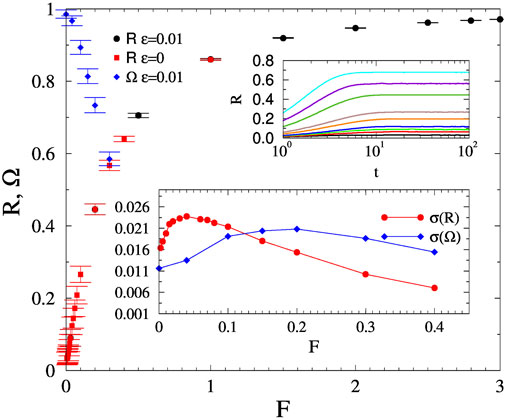
FIGURE 1. Order parameter dependence on F for the fruit-fly connectome for the noisy (black bullet) and the noiseless (red boxes) cases at K = 1.3. The blue diamonds show the steady-state Ω values with noise. Lower inset: Variances of R and Ω for the noisy case. Upper inset: Time dependence of the noisy R(t), for F = 0, 0.02, 0.03, 0.04, 0.07, 0.1, 0.2, 0.3, 0.4 (bottom to top curves).

To locate the transition we plotted the steady state values of R and Ω and their fluctuations on Figure 1. The half values provide estimates: F_c ≃ 0.22, for R and $F_c^{\prime }\simeq 0.35$ for Ω. One can see smooth fluctuation peaks of σ(R) at F ≃ 0.05 and of σ(Ω) at F′ ≃ 0.2. Thus, the two different order parameters seem to exhibit different synchronization points. The frequency fluctuation peak agrees roughly with F_c ≃ 0.22, but the phase fluctuation peak occurs at a much lower value. This, in contrast with the Hopf transition of FF and the random network, where fluctuation peaks were roughly at the same position, where we knew that the dimension is d > 4. Plotting the results on log.-log. scale it turns out that the fluctuation growth can be fitted by σ(R) ∝ F^0.16(1) for F ≤ 0.05, while following the peak, for F > 0.1, it decays as σ(R) ∝ F^−1.3(2). Thus, we have susceptibility like exponents γ′ = 0.16(1) ≠ γ = 1.3(2). Note, that in case of K = 2, when we started from a synchronous state by the addition of the force we obtained a very narrow growth region of the fluctuations, the decay is characterized by γ = 1.34(1) (see Appendix).

As σ(R) is also called SK order parameter, which characterizes the transition in excitable systems, its approach to zero as F increases agrees with the SNIC transition result of [40], albeit that was obtained in the synchronous phase. We have also run SK in the synchronous phase of FF, using K = 2, where we found similar results as in the asynchronous phase.

Results with and without a small noise with amplitude ϵ = 0.01 did not show observable differences, so the chaotic noise from the quenched disorder is capable to compete with the ordering effect of the force. We have also determined the σ(Ω(K, F)) for other K and F values, as they are close to the half values estimates of the transitions. As one can see on the inset of Figure 4 by increasing F the Kuramoto transition fluctuation peak becomes smoother and moves to smaller K values, similarly to the Widom line obtained in discrete brain models [34, 35].

As the next step we performed the same analysis of the human connectomes at K = 1, which is in the asynchronous phase without a force [57]. Figure 2 shows the steady state values both for R and Ω in case of K = 1 for KKI-113. Again the annealed noise does not modify the results and seems to be unnecessary to produce a synchronization transition. We estimated: $F_c^{\prime }\simeq 0.4$ and F_c ≃ 0.55 by the half values or R and Ω respectively. The fluctuation peaks of the two order parameters are again far away from each other: F ≃ 0.05 versus F′ ≃ 0.4. Again the fluctuation peak of Ω is close to $F_c^{\prime }\simeq 0.4$.

FIGURE 2

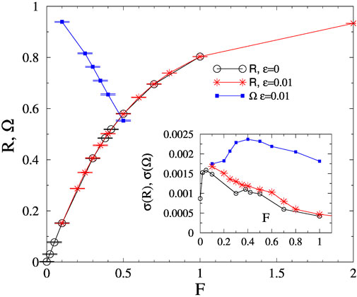
FIGURE 2. Order parameter dependence on F for the KKI-113 for the noisy and the noiseless cases at K = 1. Inset: Variances of R and Ω for the noisy case.

For the connectome KKI-18 we enlarged the fluctuation peak results on Figure 3, by comparing the noiseless and the noisy R results. The smeared synchronization ‘peaks’ happen at similar values as for KKI-113: F′ ≃ 0.05 and F ≃ 0.5 within numerical precision. The transition points, estimated by the half values of R is F_c ≃ 0.4 and of Ω is $F_c^{\prime }\simeq 0.55$. As before, the σ(R) peaks occur at much lower force values, than the other transition point estimates and the susceptibility exponents estimates have been estimated to be γ′ = 0.15(3) and γ = 1.12(2).

FIGURE 3

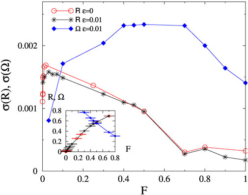
FIGURE 3. Fluctuations of R and Ω as the function of F for the KKI-18, for the noisy and the noiseless cases at K = 1. Inset: Order parameter R for the noisy and noiseless cases as well as Ω, denoted by the same symbols as in the main figure.

3.2 Avalanche durations

We investigated avalanches similarly to the local field potential experiments and as it was done in simulations of spike-like events [40]. In critical systems avalanche sizes and durations exhibit PL tails, characterized by the exponents p(S) ∝ S^−τ and $p(\mathrm{\Delta }(t))\propto \mathrm{\Delta }{(t)}^{-{\tau }_t}$. However, we did not apply thresholds for the individual variables θ_i(t), but for the global order parameter R(t). This has the advantage of a much faster algorithm, allowing us to consider larger statistics and the lack of ambiguity in the avalanche definitions [95–97]. The disadvantage is that spatially independent avalanches overlapping in time accidentally may be unified, thus the duration times can be larger and we do not have information on the spatio-temporal sizes, thus on the exponent τ. Still, we think that investigating this coarse-grained description of avalanches, which has also been measured in experiments, as a kind of crackling noise [98] in the case of zebrafish larvae [15], describes a possible critical behavior. Results of local characterization of the synchronization will be shown in Sections 3.3, 3.4, 4.2.

As in [40] here we also found that the choice of threshold T(F) value did not change the scaling behavior of the duration distributions if it was chosen within the fluctuation range R_min < T(F) < R_max corresponding to F, that was determined numerically after several runs on different initial conditions. For thresholds we used the mean value of R(t), obtained in the steady state by sample and time averaging up to t_max = 10⁴. By the integration we used uniform random distributions θ_i(0) ∈ (0, 2π) and the initial frequencies were set to be $\dot{{\theta }_i}(0)={\omega }_i^0$. Following measurements of the avalanche duration Δ(t) = t_i − t_i’, defined between subsequent crossing of an up event: R(t_i) > T and a down one: $R(t_i^{\prime })<T$, we applied a histogramming to determine the probability distributions p(Δ(t)).

Figure 4 shows the PDF p (Δ(t)) results for the fruit-fly, in case of K = 1.3, ϵ = 0.01 and different forces. We can see F dependent extended PL tails, with continuously changing exponents: 2.1 < τ_t < 2.8, which are somewhat smaller, but close to the experimental value reported for the zebrafish: τ_t = 3.0 (1) [15] and to the random field Ising model duration values [99].

FIGURE 4

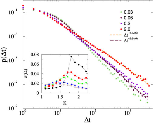
FIGURE 4. Avalanche duration distributions on the fruit-fly connectome for different forces, shown by the legends and at K = 1.3, ϵ = 0.01. Dashed lines are PL fits for Δt > 100. The inset shows the steady state σ(Ω) as the function of K, for excitation values F = 0.001, 0.0667, 0.1, 0.2, 0.3 (top to bottom).

Similar results are obtained in case of the two human connectomes as shown on Figures 5, 6. Furthermore, the results do not change without the additive noise, or in case of a force in the synchronized phase (see graphs in the Appendix).

FIGURE 5

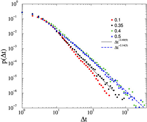
FIGURE 5. Avalanche duration distributions on the KKI-113 connectome for different forces, shown by the legends and at K = 1, ϵ = 0.01. Dashed lines are PL fits for Δt > 20. The F = 0.1 case veers down on the log.-log. scale, but for F = 0.35 a more extended PL tail with exponent τ_t = 2.40(9) can be obtained. For F = 0.4, and F = 0.5 the slopes stabilize to τ_t = 2.14(5).

FIGURE 6

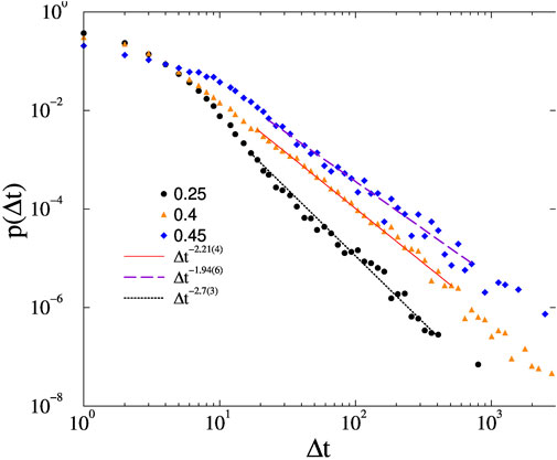
FIGURE 6. Avalanche duration distributions on the KKI-18 connectome for different forces, shown by the legends and at K = 1, ϵ = 0.01. Dashed lines are PL fits for Δt > 20.

3.3 Local order parameters snapshots

We have plotted with Wolfram Mathematica [100] snapshots of the local order parameters of the FF at different force values in increasing order for the average local parameters (see Figure 7). The giant component of the graph was plotted with 21,615 nodes, however with a very few 75,657 edges for better visualization, where we sorted the links of each node by their weights in a decreasing manner and then randomly chose the first n_r links, where n_r is a random integer between 1 and n_m = 6. Since the graph is a modular small-world graph, this kind of representation can be a close visual representation of the actual network. The color coding on the figure is a logarithmic (log₃) binned scale between 0 and 1 (0.01, 0.03, 0.09, 0.27, 0.81, 1.) representing the R_i values of each node at time step, indicated on the top left of each figure.

FIGURE 7

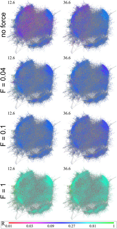
FIGURE 7. Here we see the evolution of the local order parameters R_i(t) of a sub-graph of the fruit-fly connectome at different time steps: t = 12.6, 36.6. The upper row shows R_i map without a force, the lowest one with F = 1.0. Color-coding at the bottom provides R_i(t) for all sub-figures.

Top row plots are results without force, second row at F = 0.04, third row at F = 0.1 and last row is at F = 1.0. Similarly to the β exponent’s case, we notice that the average local parameter R is not increasing linearly with the force at the same time-step. There is a maximum around 0.1, thus it does not have a linear correlation with the force. Without force the steady state has more fluctuations and the communities are more observable through visualization. By increasing the force every node comes into the same local state.

3.4 Hurst and β exponent results

The H and β exponents measure the self-similarity of a time series, when power-law behavior (10), (11) can be observed. H and β values lower than 0.5 describe anti-correlated signals. On the other hand, values between 0.5 and 1 mean signals with long range correlations in time.

First, we separated the communities in all FF, KK-18, KKI-113 connectomes with the Louvain modularity optimizing algorithm. Then, we calculated the H and β exponents for each community for the local parameters. In case of the FF the results (see Figure 8) with force could similarly be differentiated from the results without force as in the [63] experiments with rest and task driven measures. Simulation results without force seem to have longer correlations in time, resembling to the fMRI measurements at the rest phase.

FIGURE 8

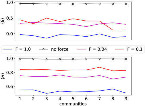
FIGURE 8. Hurst and β exponents of all fruit-fly connectome communities. In the forceless case at the critical Hopf transition coupling, the H exponent is the largest for every community. With forces these values drop for each community. This shows a resemblance with the rest and non-rest studies of different brain areas in [63], showing ⟨H⟩ ≈ 1.0 at resting state and ⟨H⟩ ≈ 0.7 at task driven states.

The same conclusion however cannot be found in the case of the human connectomes (see Figure 9). It appears that even with a relatively high force the exponents remain close to each other and close to those of the “rest” phase. In the case of FF higher force led to less “rest” in the system resembling more like task driven behaviour.

FIGURE 9

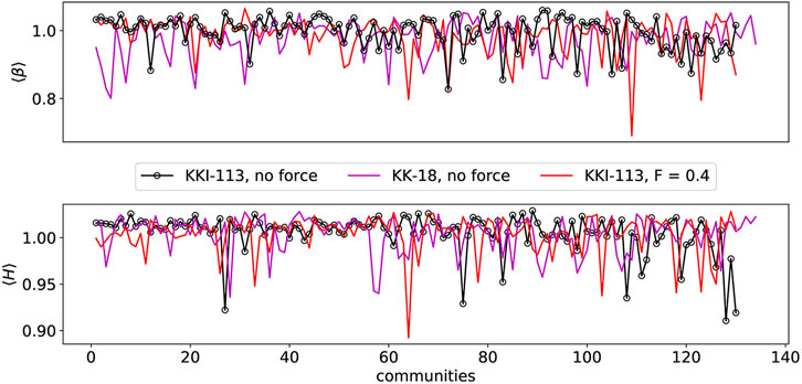
FIGURE 9. Hurst and β exponents of all human connectomes’ communities. KKI-113 is presented with and without force terms and KK-18 without the force terms.

Another very important result arose from the study of the two different human connectomes, where H exceeds the maximum value of 1. It is due to the fact that the brain at criticality is characterized by “crucial events.” Crucial events are defined as abrupt changes in the signal amplitude, for example in electroencefalogramm (EEG) signals [92]. The waiting time (τ) distribution between events follows an inverse-power law $\psi (\tau )\approx \frac{1}{{\tau }^{\mu }}$ for τ → ∞. The intermittency index μ is an important measure in the interval 1 < μ < 3, with H = (4 − μ)/2 and β = 3 − μ. The condition μ < 2 generates H > 1 with a possible maximum value H = 1.5. This is due to the fact that some non-stationary correlation could emerge in crucial events, leading to μ < 2, so that H exceeds the maximum value of 1 [93, 94]. As we can see on Figure 9, H > 1 and β > 1 occur in case of the human connectome results at certain communities, but we did not find it in the case of the FF (see Figure 8).

4 Hopf synchronization transition without force

We have rerun this analysis for the fruit-fly connectome using the standard Kuramoto equation for different couplings, i.e., near the Hopf synchronization transition discussed in [59].

4.1 Crackling noise analysis

Earlier mean-field type of phase transition was found at K_c 1.7(2). As we can see on Figure 10 the crackling noise duration analysis results in faster than PL decays of p(Δt) for K < 1.4 and an inflection point with up veering decays for K ≥ 1.65 couplings. At K = 1.5 we can observe a PDF, with PL decay for 30 < t < 300, which can be fitted by the exponent τ_t = 3.1(1). Note, that in [59] an estimate for the synchronization transition K_c = 1.70(2) was given, but in that work the RK4 solver was used mainly. Here the more precise Bulrisch-Stoer stepper was applied, which moves the p(Δ) tails slightly and provides a somewhat greater transition point estimate.

FIGURE 10

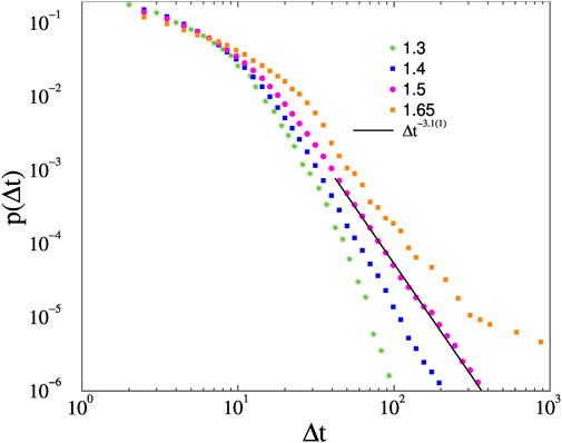
FIGURE 10. Avalanche duration distributions on the fruit-fly connectome without force for K different couplings. The line shows a PL fit for the K = 1.5 results, for Δt > 30.

As in [59] we do not find an extended scaling region with non-universal exponents suggesting a GP. So, the crackling noise exponent, presumably the mean-field class exponent of the Hopf transition, describing the resting state, should be this value. This is a rather large exponent and is difficult to reproduce by simulations, because large systems are needed to see the scaling region before an exponential cutoff. We assume that this was not seen in [40], where N = 500 nodes were used. Another reason might be that in [40] an annealed Kuramoto model was simulated, lacking the quenched self-frequencies. Or perhaps because [40] used thresholds of the θ_i(t) variables and identified avalanches by estimating the spatio-temporal size of the activity avalanches.

But indeed the scaling region we observe is rather narrow, even though we know that the Kuramoto model exhibits a critical synchronization transition here.

4.2 Hurst and β analysis of local variables

We cannot exclude the possibility that doing the avalanche analysis on the local angles θ_i(t), would lead to a lack of PL-s as it was claimed in [40]. Since identification of avalanches of local variables is a rather difficult and ambiguous task, requiring careful binning, to check the scaling of local phase and frequency data we performed auto-correlation measurements and estimated the Hurst and β exponents as before.

The “no-force” result on Figures 8, 9 show strong auto-correlations, indications of criticality as in the brain experiments [63]. In fact the exponents are larger (close to 1), than in case of the Shinomoto–Kuramoto model calculations. This suggests that the external excitation results in a less correlated scaling behavior of the neural systems than in the resting state. These results are in agreement with the experimental findings of [63].

5 Conclusion

In conclusion our numerical analysis of synchronization models on different connectome graphs show that in the case of excitation we can find PL scaling of duration of the crackling noise of the activity, defined by thresholds of R. By solving the Shinomoto-Kuramoto model numerically we concluded that even without the additive noise we can find similar synchronization transition as with the full Langevin equation.

The observed PL tails exhibit some dependence on the amplitude of the force, which may be related to GP heterogeneity effects, but can also arise as the consequence of quasi-critical, scaling like behavior reported in the discrete models of Ref. [35]. We estimated the extension of the synchronization transition region by the fluctuations of R and Ω and found an extended, smeared transition region. This makes it difficult to define the transition points. We attempted it in two different ways: half values and fluctuation peaks of the order parameters in the steady state. In general, the $F_c^{\prime }$-s, obtained by the half values of Ω are greater than the F_c-s by the R-s and agree with the frequency fluctuation peaks. While the phase fluctuations peaks were found to be much smaller both for the FF and the human connectomes. This is very different from the Kuramoto Hopf transition results [59]. The susceptibilty exponents are γ′ = 0.16(2) and γ′ = 1.3(1), but for the K = 2 case we could not measure γ′, because $F_c=F_c^{\prime }\simeq 0$ was found. The σ(Ω) results also show accordance with the Widom line, the peaks are flattened and shift by increasing the external force.

However, σ(R) also describes the transition of the SK order parameter, introduced for excitable systems. Its decay seems to be faster than the one obtained by the SNIC bifurcation at ${\omega }_i^0=1$, ϵ = 0.275 [40]. We have not reached a region, showing hybrid phase transition reported in [40], possibly by the lack of strong noise. We avoided to apply strong noise, because that makes the numerical solution less precise or very slow. A systematic finite-size scaling study of this transition would be necessary to settle this issue.

In case of initial conditions with random phase variables the R(t) curves at the transition point do not show PL growth as in case of the Kuramoto model, but a logarithmic growth, similar to strong random fixed points of models of statistical physics.

We also investigated the local order parameters and found frustrated synchronization with Chimera like states, coexistence of synchronized and asynchronous domains. Performing auto-correlation analysis on the local order parameters we found strong auto-correlation in the resting (Kuramoto) state at criticality and somewhat weaker ones in presence of an external force. In the latter case the H and β exponents take their maximal values, where the fluctuations of R(t) are maximal, i. e., at the transition.

We also investigated the module dependence of H and β by decomposing the connectomes via community detection algorithms. We observed variations amongst the communities suggesting different levels of criticality, but the identification of communities with real brain regions is a further task to be completed. Our simulated H and β exponents are in agreement with recent experimental findings [63].

Data availability statement

The raw data supporting the conclusion of this article will be made available by the authors, without undue reservation.

Author contributions

GÓ conceived of the presented idea, developed the theory. GÓ, IP, and SD performed the calculations, carried out the simulations. GÓ, IP, and SD drafted the manuscript and designed figures. JK developed the GPU codes for simulations and critically reviewed the manuscript.

Funding

Support from the Hungarian National Research, Development and Innovation Office NKFIH (K128989) is acknowledged.

Acknowledgments

We thank Gustavo Deco and Gerarardo Ortiz for the useful comments. Most of the numerical work was done on KIFU supercomputers of Hungary.

Conflict of interest

The authors declare that the research was conducted in the absence of any commercial or financial relationships that could be construed as a potential conflict of interest.

Publisher’s note

All claims expressed in this article are solely those of the authors and do not necessarily represent those of their affiliated organizations, or those of the publisher, the editors and the reviewers. Any product that may be evaluated in this article, or claim that may be made by its manufacturer, is not guaranteed or endorsed by the publisher.

References

1. Beggs J, Plenz D. Neuronal avalanches in neocortical circuits. J Neurosci (2003) 23:11167–77. doi:10.1523/jneurosci.23-35-11167.2003

PubMed Abstract | CrossRef Full Text | Google Scholar

2. Mazzoni A, Broccard FD, Garcia-Perez E, Bonifazi P, Ruaro ME, Torre V. On the dynamics of the spontaneous activity in neuronal networks. PLoS One (2007) 2:e439. doi:10.1371/journal.pone.0000439

PubMed Abstract | CrossRef Full Text | Google Scholar

3. Pasquale V, Massobrio P, Bologna L, Chiappalone M, Martinoia S. Self-organization and neuronal avalanches in networks of dissociated cortical neurons. Neuroscience (2008) 153:1354–69. doi:10.1016/j.neuroscience.2008.03.050

PubMed Abstract | CrossRef Full Text | Google Scholar

4. Friedman N, Ito S, Brinkman BAW, Shimono M, DeVille REL, Dahmen KA, et al. Universal critical dynamics in high resolution neuronal avalanche data. Phys Rev Lett (2012) 108:208102. doi:10.1103/physrevlett.108.208102

PubMed Abstract | CrossRef Full Text | Google Scholar

5. Hahn G, Petermann T, Havenith MN, Yu S, Singer W, Plenz D, et al. Neuronal avalanches in spontaneous activity in vivo. J Neurophysiol (2010) 104:3312–22. pMID: 20631221. doi:10.1152/jn.00953.2009

PubMed Abstract | CrossRef Full Text | Google Scholar

6. Shriki O, Alstott J, Carver F, Holroyd T, Henson RN, Smith ML, et al. Neuronal avalanches in the resting MEG of the human brain. J Neurosci (2013) 33:7079–90. doi:10.1523/jneurosci.4286-12.2013

PubMed Abstract | CrossRef Full Text | Google Scholar

7. Tagliazucchi E, Balenzuela P, Fraiman D, Chialvo D. Criticality in large-scale brain FMRI dynamics unveiled by a novel point process analysis. Front Physiol (2012) 3:15. doi:10.3389/fphys.2012.00015

PubMed Abstract | CrossRef Full Text | Google Scholar

8. Scott G, Fagerholm ED, Mutoh H, Leech R, Sharp DJ, Shew WL, et al. Voltage imaging of waking mouse cortex reveals emergence of critical neuronal dynamics. J Neurosci (2014) 34:16611–20. doi:10.1523/jneurosci.3474-14.2014

PubMed Abstract | CrossRef Full Text | Google Scholar

9. Priesemann V, Wibral M, Valderrama M, Pröpper R, Le Van Quyen M, Geisel T, et al. Front Syst Neurosci (2014) 8:108.

PubMed Abstract |

10. Bellay T, Klaus A, Seshadri S, Plenz D. Elife (2015) 4:e07224.

PubMed Abstract |

11. Hahn G, Ponce-Alvarez A, Monier C, Benvenuti G, Kumar A, Chavane F, et al. Spontaneous cortical activity is transiently poised close to criticality. PLOS Comput Biol (2017) 13:e1005543. doi:10.1371/journal.pcbi.1005543

PubMed Abstract | CrossRef Full Text | Google Scholar

12. Seshadri S, Klaus A, Winkowski D, Kanold PO, Plenz D. Altered avalanche dynamics in a developmental NMDAR hypofunction model of cognitive impairment. Transl Psychiatry (2018) 8:3. doi:10.1038/s41398-017-0060-z

PubMed Abstract | CrossRef Full Text | Google Scholar

13. Palva J, Zhigalov A, Hirvonen J, Korhonen O, Linkenkaer-Hansen K, Palva S. Neuronal long-range temporal correlations and avalanche dynamics are correlated with behavioral scaling laws. Proc Natl Acad Sci United States America (2013) 110:3585–90. doi:10.1073/pnas.1216855110

PubMed Abstract | CrossRef Full Text | Google Scholar

14. Fuscà M, Siebenhühner F, Wang SH, Myrov V, Arnulfo G, Nobili L, et al. Brain criticality predicts individual synchronization levels in humans. bioRxiv (2022). doi:10.1101/2022.11.24.517800

CrossRef Full Text | Google Scholar

15. Ponce-Alvarez A, Jouary A, Privat M, Deco G, Sumbre G. Whole-brain neuronal activity displays crackling noise dynamics. Neuron (2018) 100:1446–59.e6. doi:10.1016/j.neuron.2018.10.045

PubMed Abstract | CrossRef Full Text | Google Scholar

16. Yaghoubi M, De Graaf T, Orlandi J, Girotto F, Colicos M, Davidsen J. Neuronal avalanche dynamics indicates different universality classes in neuronal cultures. Scientific Rep (2018) 8:3417. doi:10.1038/s41598-018-21730-1

PubMed Abstract | CrossRef Full Text | Google Scholar

17. Chialvo D, Bak P. Learning from mistakes. Neuroscience (1999) 90:1137–48. doi:10.1016/s0306-4522(98)00472-2

PubMed Abstract | CrossRef Full Text | Google Scholar

18. Chialvo DR. complexity and criticality: In memory of per bak. Physica A: Stat Mech its Appl (2004) 340:7561947–2002.

Google Scholar

19. Chialvo DR. Are our senses critical? Nat Phys (2006) 2:301–2. doi:10.1038/nphys300

CrossRef Full Text | Google Scholar

20. Chialvo DR. The brain near the edge. AIP Conf Proc (2007) 887:1. doi:10.1063/1.2709580

CrossRef Full Text | Google Scholar

21. Chialvo DR, Balenzuela P, Fraiman D. The brain: What is critical about it? AIP Conf Proc (2008) 1028:28. doi:10.1063/1.2965095

CrossRef Full Text | Google Scholar

22. Fraiman D, Balenzuela P, Foss J, Chialvo DR. Ising-like dynamics in large-scale functional brain networks. Phys Rev E (2009) 79:061922. doi:10.1103/physreve.79.061922

PubMed Abstract | CrossRef Full Text | Google Scholar

23. Expert P, Lambiotte R, Chialvo DR, Christensen K, Jensen HJ, Sharp DJ, et al. Self-similar correlation function in brain resting-state functional magnetic resonance imaging. J R Soc Interf (2011) 8:472–9. doi:10.1098/rsif.2010.0416

PubMed Abstract | CrossRef Full Text | Google Scholar

24. Fraiman D, Chialvo D. What kind of noise is brain noise: Anomalous scaling behavior of the resting brain activity fluctuations. Front Physiol (2012) 3:307. doi:10.3389/fphys.2012.00307

PubMed Abstract | CrossRef Full Text | Google Scholar

25. Deco G, Jirsa VK. Ongoing cortical activity at rest: Criticality, multistability, and ghost attractors. J Neurosci (2012) 32:3366–75. doi:10.1523/jneurosci.2523-11.2012

PubMed Abstract | CrossRef Full Text | Google Scholar

26. Deco G, Ponce-Alvarez A, Hagmann P, Romani G, Mantini D, Corbetta M. How local excitation-inhibition ratio impacts the whole brain dynamics. J Neurosci (2014) 34:7886–98. doi:10.1523/jneurosci.5068-13.2014

PubMed Abstract | CrossRef Full Text | Google Scholar

27. Senden M, Reuter N, van den Heuvel MP, Goebel R, Deco G. Cortical rich club regions can organize state-dependent functional network formation by engaging in oscillatory behavior. NeuroImage (2017) 146:561–74. doi:10.1016/j.neuroimage.2016.10.044

PubMed Abstract | CrossRef Full Text | Google Scholar

28. Muñoz MA. Colloquium: Criticality and dynamical scaling in living systems. Rev Mod Phys (2018) 90:031001. doi:10.1103/RevModPhys.90.031001

CrossRef Full Text | Google Scholar

29. Plenz D, Ribeiro TL, Miller SR, Kells PA, Vakili A, Capek EL. Self-organized criticality in the brain. Front Phys (2021) 9:365. doi:10.3389/fphy.2021.639389

CrossRef Full Text | Google Scholar

30. Kinouchi O, Copelli M. Optimal dynamical range of excitable networks at criticality. Nat Phys (2006) 2:348–51. doi:10.1038/nphys289

CrossRef Full Text | Google Scholar

31. Bak P, Tang C, Wiesenfeld K. Self-organized criticality: An explanation of the 1/fnoise. Phys Rev Lett (1987) 59:381–4. doi:10.1103/physrevlett.59.381

PubMed Abstract | CrossRef Full Text | Google Scholar

32. Vojta T. Rare region effects at classical, quantum and nonequilibrium phase transitions. J Phys A: Math Gen (2006) 39:R143–205. doi:10.1088/0305-4470/39/22/r01

CrossRef Full Text | Google Scholar

33. Ódor G, Gastner MT, Kelling J, Deco G. Modelling on the very large-scale connectome. J Phys Complexity (2021) 2:045002. doi:10.1088/2632-072x/ac266c

CrossRef Full Text | Google Scholar

34. Williams-García RV, Moore M, Beggs JM, Ortiz G. Quasicritical brain dynamics on a nonequilibrium Widom line. Phys Rev E (2014) 90:062714. doi:10.1103/PhysRevE.90.062714

CrossRef Full Text | Google Scholar

35. Fosque LJ, Williams-García RV, Beggs JM, Ortiz G. Evidence for quasicritical brain dynamics. Phys Rev Lett (2021) 126:098101. doi:10.1103/physrevlett.126.098101

PubMed Abstract | CrossRef Full Text | Google Scholar

36. Korchinski DJ, Orlandi JG, Son S-W, Davidsen J. Criticality in spreading processes without timescale separation and the critical brain hypothesis. Phys Rev X (2021) 11:021059. doi:10.1103/PhysRevX.11.021059

CrossRef Full Text | Google Scholar

37. Almeira J, Grigera TS, Chialvo DR, Cannas SA. Tricritical behavior in a neural model with excitatory and inhibitory units. Phys Rev E (2022) 106:054140. doi:10.1103/PhysRevE.106.054140

PubMed Abstract | CrossRef Full Text | Google Scholar

38. Ódor G, de Simoni B. Heterogeneous excitable systems exhibit Griffiths phases below hybrid phase transitions. Phys Rev Res (2021) 3:013106. doi:10.1103/physrevresearch.3.013106

CrossRef Full Text | Google Scholar

39. Corral López R, Buendía V, Muñoz MA. Excitatory-inhibitory branching process: A parsimonious view of cortical asynchronous states, excitability, and criticality. Phys Rev Res (2022) 4:L042027. doi:10.1103/PhysRevResearch.4.L042027

CrossRef Full Text | Google Scholar

40. Buendía V, Villegas P, Burioni R, Muñoz MA. Hybrid-type synchronization transitions: Where incipient oscillations, scale-free avalanches, and bistability live together. Phys Rev Res (2021) 3:023224. doi:10.1103/PhysRevResearch.3.023224

CrossRef Full Text | Google Scholar

41. Morales GB, Di Santo S, Muñoz MA. Unifying model for three forms of contextual modulation including feedback input from higher visual areas. bioRxiv (2022). doi:10.1101/2022.05.27.493753v1

CrossRef Full Text | Google Scholar

42. Ye X, Vojta T. Contact process with simultaneous spatial and temporal disorder. Phys Rev E (2022) 106:044102. doi:10.1103/PhysRevE.106.044102

PubMed Abstract | CrossRef Full Text | Google Scholar

43. Ódor G. Robustness of Griffiths effects in homeostatic connectome models. Phys Rev E (2019) 99:012113. doi:10.1103/PhysRevE.99.012113

PubMed Abstract | CrossRef Full Text | Google Scholar

44. Griffiths RB. Nonanalytic behavior above the critical point in a random ising ferromagnet. Phys Rev Lett (1969) 23:17–9. doi:10.1103/physrevlett.23.17

CrossRef Full Text | Google Scholar

45. Moretti P, Muñoz MA. Griffiths phases and the stretching of criticality in brain networks. Nat Commun (2013) 4:2521. doi:10.1038/ncomms3521

PubMed Abstract | CrossRef Full Text | Google Scholar

46. Ódor G, Dickman R, Ódor G. Griffiths phases and localization in hierarchical modular networks. Scientific Rep (2015) 5:14451. doi:10.1038/srep14451

CrossRef Full Text | Google Scholar

47. Cota W, Ódor G, Ferreira SC. Griffiths phases in infinite-dimensional, non-hierarchical modular networks. Scientific Rep (2018) 8:9144. doi:10.1038/s41598-018-27506-x

PubMed Abstract | CrossRef Full Text | Google Scholar

48. Buendí a V, Villegas P, Burioni R, Muñoz MA. The broad edge of synchronization: Griffiths effects and collective phenomena in brain networks. Philos Trans R Soc A: Math Phys Eng Sci (2022) 380:20200424. doi:10.1098/rsta.2020.0424

CrossRef Full Text | Google Scholar

49. Cota W, Ferreira SC, Ódor G. Griffiths effects of the susceptible-infected-susceptible epidemic model on random power-law networks. Phys Rev E (2016) 93:032322. doi:10.1103/physreve.93.032322

PubMed Abstract | CrossRef Full Text | Google Scholar

50. Burkitt AN. A review of the integrate-and-fire neuron model: I. Homogeneous synaptic input. Biol Cybernetics (2006) 95:1–19. ISSN 1432-0770. doi:10.1007/s00422-006-0068-6

PubMed Abstract | CrossRef Full Text | Google Scholar

51. Liang J, Zhou T, Zhou C. Hopf bifurcation in mean field explains critical avalanches in excitation-inhibition balanced neuronal networks: A mechanism for multiscale variability. Front Syst Neurosci (2020) 14. ISSN 1662-5137. doi:10.3389/fnsys.2020.580011

CrossRef Full Text | Google Scholar

52. Orlandi JG, Soriano J, Alvarez-Lacalle E, Teller S, Casademunt J. Noise focusing and the emergence of coherent activity in neuronal cultures. Nat Phys (2013) 9:582–90. doi:10.1038/nphys2686

CrossRef Full Text | Google Scholar

53. Janssen HK. On the nonequilibrium phase transition in reaction-diffusion systems with an absorbing stationary state. Z Phys B (1981) 42:151–4. doi:10.1007/bf01319549

CrossRef Full Text | Google Scholar

54. Grassberger P. On phase transitions in Schlögl's second model. Z Phys B (1982) 47:365–74. doi:10.1007/bf01313803

CrossRef Full Text | Google Scholar

55. Ódor G. Universality in nonequilibrium lattice systems: Theoretical foundations. Singapore: World Scientific (2008).

Google Scholar

56. Ódor G. Stochastic resetting in backtrack recovery by RNA polymerases. Phys Rev E (2016) 94:062411. doi:10.1103/PhysRevE.93.062411

PubMed Abstract | CrossRef Full Text | Google Scholar

57. Ódor G, Kelling J. Critical synchronization dynamics of the Kuramoto model on connectome and small world graphs. Scientific Rep (2019) 9:19621. doi:10.1038/s41598-019-54769-9

CrossRef Full Text | Google Scholar

58. Ódor G, Kelling J, Deco G. The effect of noise on the synchronization dynamics of the Kuramoto model on a large human connectome graph. J Neurocomputing (2021) 461:696–704. doi:10.1016/j.neucom.2020.04.161

CrossRef Full Text | Google Scholar

59. Ódor G, Deco G, Kelling J. Differences in the critical dynamics underlying the human and fruit-fly connectome. Phys Rev Res (2022) 4:023057. doi:10.1103/PhysRevResearch.4.023057

CrossRef Full Text | Google Scholar

60. Villegas P, Moretti P, Muñoz M. Frustrated hierarchical synchronization and emergent complexity in the human connectome network. Scientific Rep (2014) 4:5990. doi:10.1038/srep05990

PubMed Abstract | CrossRef Full Text | Google Scholar

61. Villegas P, Hidalgo J, Moretti P, Muñoz M. Proceedings of ECCS 2014: European conference on complex systems (2016). p. 69–80.

CrossRef Full Text | Google Scholar

62. Millán A, Torres J, Bianconi G. Complex network geometry and frustrated synchronization. Scientific Rep (2018) 8:9910. doi:10.1038/s41598-018-28236-w

CrossRef Full Text | Google Scholar

63. Ochab JK, Wa̧torek M, Ceglarek A, Fafrowicz M, Lewandowska K, Marek T, et al. Task-dependent fractal patterns of information processing in working memory. Scientific Rep (2022) 12:17866. ISSN 2045-2322. doi:10.1038/s41598-022-21375-1

CrossRef Full Text | Google Scholar

64. Kuramoto Y. Chemical oscillations, waves, and turbulence, springer series in synergetics. Berlin, Heidelberg: Springer Berlin Heidelberg (2012). ISBN 9783642696893.

Google Scholar

65. Shinomoto S, Kuramoto Y. Phase transitions in active rotator systems. Prog Theor Phys (1986) 75:1105–10. ISSN 0033-068X. doi:10.1143/ptp.75.1105

CrossRef Full Text | Google Scholar

66. Sakaguchi H. Cooperative phenomena in coupled oscillator systems under external fields. Prog Theor Phys (1988) 79:39–46. doi:10.1143/ptp.79.39

CrossRef Full Text | Google Scholar

67. Antonsen TM, Faghih RT, Girvan M, Ott E, Platig J. External periodic driving of large systems of globally coupled phase oscillators. Chaos: Interdiscip J Nonlinear Sci (2008) 18:037112. doi:10.1063/1.2952447

PubMed Abstract | CrossRef Full Text | Google Scholar

68. Ott E, Antonsen TM. Low dimensional behavior of large systems of globally coupled oscillators. Chaos: Interdiscip J Nonlinear Sci (2008) 18:037113. doi:10.1063/1.2930766

PubMed Abstract | CrossRef Full Text | Google Scholar

69. Childs LM, Strogatz SH. Stability diagram for the forced Kuramoto model. Chaos: Interdiscip J Nonlinear Sci (2008) 18:043128. doi:10.1063/1.3049136

PubMed Abstract | CrossRef Full Text | Google Scholar

70. Deuflhard P. Order and stepsize control in extrapolation methods. Numerische Mathematik (1983) 41:399–422. doi:10.1007/bf01418332

CrossRef Full Text | Google Scholar

71. Hairer E, Norsett SP, Wanner G. Solving ordinary differential equations I. In: Nonstiff problems. In: Vol. 8 of springer series in comput. Mathematics. 2nd ed. Berlin, Heidelberg: Springer-Verlag (1987).

CrossRef Full Text | Google Scholar

72. Maruyama G. Continuous Markov processes and stochastic equations. Rendiconti Del Circolo Matematico di Palermo (1955) 4:48. ISSN 1973-90. doi:10.1007/BF02846028

CrossRef Full Text | Google Scholar

73. Lima Dias Pinto I, Copelli M. Oscillations and collective excitability in a model of stochastic neurons under excitatory and inhibitory coupling. Phys Rev E (2019) 100:062416. doi:10.1103/physreve.100.062416

PubMed Abstract | CrossRef Full Text | Google Scholar

74. Sporns O, Tononi G, Kötter R. The human connectome: A structural description of the human brain. PLOS Comput Biol (2005) 1:e42. doi:10.1371/journal.pcbi.0010042

PubMed Abstract | CrossRef Full Text | Google Scholar

75.The hemibrain dataset. The hemibrain dataset (v1.0.1) (2020). Available from: https://storage.cloud.google.com/hemibrain-release/neuprint/hemibrain_v1.0.1_neo4j_inputs.zip (Accessed January 23, 2020).

Google Scholar

76. Landman BA, Huang AJ, Gifford A, Vikram DS, Lim IAL, Farrell JAD, et al. Multi-parametric neuroimaging reproducibility: A 3-T resource study. NeuroImage (2011) 54:2854–66. doi:10.1016/j.neuroimage.2010.11.047

PubMed Abstract | CrossRef Full Text | Google Scholar

77. Delettre C, Messé A, Dell L-A, Foubet O, Heuer K, Larrat B, et al. Comparison between diffusion MRI tractography and histological tract-tracing of cortico-cortical structural connectivity in the ferret brain. Netw Neurosci (2019) 3:1038–50. doi:10.1162/netn_a_00098

PubMed Abstract | CrossRef Full Text | Google Scholar

78. Gastner MT, Ódor G. The topology of large Open Connectome networks for the human brain. Scientific Rep (2016) 6:27249. doi:10.1038/srep27249

PubMed Abstract | CrossRef Full Text | Google Scholar

79.Neurodata. Neurodata (2015). Available from: https://neurodata.io (Accessed October 2, 2015).

Google Scholar

80. Gray Roncal W, Koterba ZH, Mhembere D, Kleissas DM, Vogelstein JT, Burns R, et al. Migraine: MRI graph reliability analysis and inference for connectomics. In: 2013 IEEE Global Conference on Signal and Information Processing (2013). p. 313–6.

CrossRef Full Text | Google Scholar

81.Docker Hub. Neurodata/m2g (2023). Available from: https://hub.docker.com/r/neurodata/m2g/builds.

Google Scholar

82. Desikan RS, Ségonne F, Fischl B, Quinn BT, Dickerson BC, Blacker D, et al. An automated labeling system for subdividing the human cerebral cortex on MRI scans into gyral based regions of interest. NeuroImage (2006) 31:968–80. doi:10.1016/j.neuroimage.2006.01.021

PubMed Abstract | CrossRef Full Text | Google Scholar

83. Klein A, Tourville J. 101 labeled brain images and a consistent human cortical labeling protocol. Front Neurosci (2012) 6:171. doi:10.3389/fnins.2012.00171

PubMed Abstract | CrossRef Full Text | Google Scholar

84. Newman MEJ. Modularity and community structure in networks. Proc Natl Acad Sci U S A (2006) 103:8577–82. doi:10.1073/pnas.0601602103

PubMed Abstract | CrossRef Full Text | Google Scholar

85. Blondel VD, Guillaume J-L, Lambiotte R, Lefebvre E. Fast unfolding of communities in large networks. J Stat Mech Theor Exp (2008) 2008:P10008. doi:10.1088/1742-5468/2008/10/p10008

CrossRef Full Text | Google Scholar

86. Humphries MD, Gurney K. Network ‘small-world-ness’: A quantitative method for determining canonical network equivalence. PLoS One (2008) 3:e0002051. doi:10.1371/journal.pone.0002051

PubMed Abstract | CrossRef Full Text | Google Scholar

87. Restrepo JG, Ott E, Hunt BR. Onset of synchronization in large networks of coupled oscillators. Phys Rev E (2005) 71:036151. doi:10.1103/physreve.71.036151

PubMed Abstract | CrossRef Full Text | Google Scholar

88. Schröder M, Timme M, Witthaut D. A universal order parameter for synchrony in networks of limit cycle oscillators. Chaos: Interdiscip J Nonlinear Sci (2017) 27:073119. doi:10.1063/1.4995963

CrossRef Full Text | Google Scholar

89. Sanchez-Rodriguez LM, Iturria-Medina Y, Mouches P, Sotero RC. Detecting brain network communities: Considering the role of information flow and its different temporal scales. NeuroImage (2021) 225:117431. ISSN 1053-8119. doi:10.1016/j.neuroimage.2020.117431

PubMed Abstract | CrossRef Full Text | Google Scholar

90. Deritei D, Lázár ZI, Papp I, Járai-Szabó F, Sumi R, Varga L, et al. Community detection by graph Voronoi diagrams. New J Phys (2014) 16:063007. doi:10.1088/1367-2630/16/6/063007

CrossRef Full Text | Google Scholar

91. Lázár ZI, Papp I, Varga L, Járai-Szabó F, Deritei D, Ercsey-Ravasz M. Stochastic graph Voronoi tessellation reveals community structure. Phys Rev E (2017) 95:022306. doi:10.1103/PhysRevE.95.022306

PubMed Abstract | CrossRef Full Text | Google Scholar

92. Allegrini P, Paradisi P, Menicucci D, Gemignani A. Fractal complexity in spontaneous EEG metastable-state transitions: New vistas on integrated neural dynamics. Front Physiol (2010) 1. ISSN 1664-042X. doi:10.3389/fphys.2010.00128

PubMed Abstract | CrossRef Full Text | Google Scholar

93. Kalashyan AK, Buiatti M, Grigolini P. Ergodicity breakdown and scaling from single sequences. Chaos, Solitons and Fractals (2009) 39:895–909. doi:10.1016/j.chaos.2007.01.062

CrossRef Full Text | Google Scholar

94. Buiatti M, Papo D, Baudonnière P-M, van Vreeswijk C. Feedback modulates the temporal scale-free dynamics of brain electrical activity in a hypothesis testing task. Neuroscience (2007) 146:1400–12. ISSN 0306-4522. doi:10.1016/j.neuroscience.2007.02.048

PubMed Abstract | CrossRef Full Text | Google Scholar

95. Touboul J, Destexhe A. Can power-law scaling and neuronal avalanches arise from stochastic dynamics? PloS one (2010) 5:e8982. doi:10.1371/journal.pone.0008982

PubMed Abstract | CrossRef Full Text | Google Scholar

96. Villegas P, Di Santo S, Burioni R, Muñoz MA. Time-series thresholding and the definition of avalanche size. Phys Rev E (2019) 100:012133. doi:10.1103/physreve.100.012133

PubMed Abstract | CrossRef Full Text | Google Scholar

97. Dalla Porta L, Copelli M. Modeling neuronal avalanches and long-range temporal correlations at the emergence of collective oscillations: Continuously varying exponents mimic M/EEG results. PLoS Comput Biol (2019) 15:e1006924. doi:10.1371/journal.pcbi.1006924

PubMed Abstract | CrossRef Full Text | Google Scholar

98. Sethna JP, Dahmen KA, Myers CR. Crackling noise. Nature (2001) 410:242–50. doi:10.1038/35065675

PubMed Abstract | CrossRef Full Text | Google Scholar

99. Sethna JP, Dahmen KA, Perkovic O. Random-field ising models of hysteresis. In: G Bertotti, and ID Mayergoyz, editors. The science of hysteresis. Oxford: Academic Press (2006). p. 107–79. ISBN 978-0-12-480874-4. doi:10.1016/B978-012480874-4/50013-0

CrossRef Full Text | Google Scholar

100. Research W. Graph (2022). Available from: https://reference.wolfram.com/language/ref/Graph.html (Accessed June 29, 2022).

Google Scholar

APPENDIX

Here we show avalanche duration PDF-s without noise in case of the KKI-113 connectome on Appendix figure A1. One see only a slight variation of the PL tail exponents around −2.2, but they are close to the noisy case results.

FIGURE A1

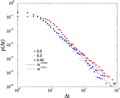
FIGURE A1. Avalanche duration distributions on the KKI-113 connectome for different forces, shown by the legends and at K = 1, without noise. Dashed lines are PL fits for Δt > 20.

Similarly, in case of the FF with the application of force in the synchronized phase, i.e., K = 2 the PL tails fitted for t > 20 do not differ to much, they can be characterized by an exponent −2.21(1) as one can see on Appendix figure A2. The inset shows the rapid drop of the SK order parameter as the function of the force and the maximum both of σ(R), σ(Ω) are at F ≃ 0. Plotting the F dependence of σ(R) on log.-log. scale a PL tail arises, characterized by the exponent −1.34(1), which can be regarded a susceptibilty exponent of the Kuramoto equations. However, σ(Ω) falls exponentially fast as the function of F.

FIGURE A2

FIGURE A2. Avalanche duration distributions on the fruit-fly connectome for different forces, shown by the legends and at K = 2, ϵ = 0.01. Dashed lines are PL fits for Δt > 100. The inset shows σ(R) by increasing F on log. log. scale. The line corresponds to a PL fit.