 M. Lapenna1
 R. Fioresi
- 1DIFA, University of Bologna, Bologna, Italy
- 2Dipartimento di Scienze Chimiche e Geologiche, University of Modena and Reggio Emilia, Modena, Italy
- 3FaBiT, University of Bologna, Bologna, Italy
We analyse the dynamics of convolutional filters’ parameters of a convolutional neural networks during and after training, via a thermodynamic analogy which allows for a sound definition of temperature. We show that removing high temperature filters has a minor effect on the performance of the model, while removing low temperature filters influences majorly both accuracy and loss decay. This result could be exploited to implement a temperature-based pruning technique for the filters and to determine efficiently the crucial filters for an effective learning.
1 Introduction
Deep Learning and neural networks [2–4] are among the most successful tools in machine learning. In recent years, the research was mainly driven by a practical point of view, mostly towards the improvement of the performance of the networks, without making a general effort towards a comprehensive theory to interpret and explain the results. Neural networks have largely been used as black boxes, deep and complex models able to adapt more and more precisely to data, making it more and more difficult to understand how this learning occurs. The problem of explainability of deep learning algorithms has now become an important issue to deal with in order to understand and guide the usage of this technology ([5, 6]). In this work, we would like to provide a physically inspired description of the functioning of convolutional neural networks (CNN), continuing a study we initiated in [1], where the thermodynamics language was successfully employed to establish a more stringent analogy between thermodynamic systems and neural networks. Indeed, starting from the visionary work by Jaynes [7] and Hopfield [8], the powerful machinery of thermodynamics was already, from the very beginning, a driving force in trying to interpret the mechanism of functioning of neural networks. Later on, after the interlude and successes of Boltzmann machines, Hinton proposed a CNN version in [9]. More work on the interpretation of neural networks via thermodynamics appears in [10, 11], where a modeling via the Fokker-Planck equation is introduced and the steady states of two distributions are analyzed in connection with the stochastic gradient descent (SGD) optimization. Along the same vein, in [12, 13] more mathematical modeling on SGD comes via the Langevin equation and gravity formalisms, in the weak field approximation, respectively. Also, a notable attempt to a more geometrical modeling in machine learning via thermodynamic concepts appears in the Lie group thermodynamic approach originally due to Souriau, see [14] and refs. therein.
Besides theoretical interest, we exploit the thermodynamic analogy to reduce the computational and storage cost of the network by introducing a temperature-based pruning technique for the filters. Pruning of CNN filter weights is a common practice, since such layers carry the major computational cost in the training of a CNN architecture. In particular, compared to pruning weights across the network, filter pruning is a naturally structured way of pruning without introducing sparsity ([15, 16]). In Sec. 2, we will make a comparison between our temperature-based pruning technique for the filters and the magnitude-based pruning of [16].
In the present paper, we look at a neural network as a dynamical system and we want to understand the dynamics of its parameters during and after the training. We model the set of parameters as non-quantum and non-relativistic particles and we link the time evolution of the trajectories to concepts from thermodynamics and molecular dynamics. In our experiments we focus on CNNs and we study the behaviour of the parameters of each filter of the CNN separately. Our experiments show how the physical interpretation sheds light on the behaviour of this system and forms the basis for future improvements of our understanding of it.
In Sec. 1 we give some physical interpretation of stochastic gradient descent during training and we introduce the analogy with thermodynamics, in particular the concept of temperature (see also [1, 10]).
In Sec. 2 we describe our key experiment, where we remove filters depending on their temperature and look at the resulting metrics of the model (accuracy and loss). We discover that “hot” filters can be pruned without affecting the performance.
Inspired by this first result, in Sec. 3 we further deepen our understanding through experiments regarding the dynamics of the parameters at equilibrium. We discover that higher temperature for the filter is due to weights oscillating more and reaching more distant positions. Furthermore, we are also interested in discovering the general characteristics of the dynamics under SGD and we find out a double component dynamics for the weights.
Finally, in Sec. 5, we draw conclusions and we mention further directions for the future.
1.1 Deep learning and thermodynamics
We review, compare and deepen the study of the thermodynamic analysis of SGD in [1, 10].
1.1.1 Stochastic gradient descent (SGD)
In a problem of optimization, a standard technique to minimize the loss function L is the gradient descent (GD) with respect to the weights w, that are the parameters defining our model. The update step in the space of parameters has the form:
where η is the learning rate and it is an hyperparameter of the model, i.e., chosen during validation.
The gradient descent minimization technique is guaranteed to reach a suitable minimum of the loss function only if such function is convex. Since in real experiments involving neural networks the loss function is usually a non-convex function, it is necessary to use a variation of GD, namely, stochastic gradient descent (SGD). In SGD, we do not compute the gradient of the loss function summing over all training data, but only on a randomly chosen subset of training samples, called minibatch,
where M is the size of the dataset, while
In SGD the samples are extracted randomly and the same sample can be extracted more than once in subsequent steps. This stochastic technique of learning allows to explore the landscape of the loss function with a noisy movement around the direction of steepest descent and this prevents the training dynamics from being trapped in an inconvenient local minimum of the loss function. We define as epoch the number of steps of training necessary to cover a number of samples equal to the size of the entire training set.
1.1.2 Stochastic differential equations and SGD
We briefly review the work [10], since we want to generalize some concepts appearing there and make a comparison with our work. In [10], Chaudhari and Soatto propose a model for the discrete SGD updates via a stochastic differential equation (SDE). The continuous time limit of SGD is expressed as the equation:
where W(t) is introduced to take into account the stochasticity of the descent. In the original treatment by Ito ([17] and refs. therein), W is modeling a Wiener process, as Brownian motion, and D(w), the diffusion matrix, controls the anisotropy of the diffusivity in the process. In our setting, it is the covariance matrix of the gradient of the loss and, in the experiments with SGD, it shows a very low rank: this is due to the highly non-isotropic nature of the gradient of the loss functions typically chosen in CNNs (see also [13]).
In [10], ζ is called the temperature and it is defined as
Due to the anisotropy of the SGD, in [10], the authors argue that what is effectively minimized during the training of the neural network is not the original loss function L, but an implicit potential ϕ exhibiting different critical points. The distribution ρ of the weights is stated to evolve according to the following Fokker-Planck equation, which is a deterministic partial differential equation:
with a unique steady-state distribution which satisfies
where Z(ζ) is a normalizing function, which resembles the partition function from statistical mechanics. SGD hence implicitly minimizes a combination of two terms: one “energetic” and the other “entropic”. The steady-state of SGD dynamics is such that it places most of its probability in regions of the parameter space with small values of ϕ(w), while maximizing the entropy of the distribution ρss(w). The entropic term captures the non-equilibrium behaviour of SGD, which, precisely because of this, is able to obtain a good generalization performance. We will make an analogy between this double component potential and the double component dynamics of the weights we find out in Sec. 3. As found in [19], solutions of discrete learning problems providing good generalization belong to dense clusters in the parameters space, rather than to sharp local minima. Chaudhari and Soatto exploit this observation and construct a loss that is a smoothed version of the original loss. Instead of relying on non-isotropic gradient noise to obtain out-of-equilibrium behavior, these well-generalizable solutions are found by construction. That is the same aim of [20], where a local-entropy-based objective function is proposed, in order to favoring well-generalizable solutions lying in large flat regions of the energy landscape, while avoiding poorly-generalizable solutions located in the sharp valleys.
1.1.3 Temperature of a neural network
In [1], Fioresi, Faglioni, Morri and Squadrani introduce a parallelism between the SGD dynamics of the weights and the kinetic theory of a gas of particles. Indeed, it is not difficult to imagine the large number of weights of the network as particles interacting with each other. They compute the temperature ζ for different layers of a convolutional architecture, by proposing an operational definition of it through a thermodynamic analogy. First of all, each parameter is thought as a particle with unitary mass and its scalar value is considered as its position. The instantaneous velocity of the parameter is defined as the difference between the value of the parameter at one step of training and its value at the previous step:
The authors define the instantaneous temperature of the system as the mean kinetic energy of the particles:
where N is the number of particles, or of degrees of freedom, and kB is a constant to match the desired units. The thermodynamic temperature at equilibrium, i.e., at the equilibrium of accuracy and loss, is then defined as the time average of T(t) over the time steps:
where
Given this definition of temperature, the authors measure it directly on the layers of a modified LeNet architecture consisting of two convolutional layers followed by two linear ones. Specifically, they compute the temperature on the last epoch of training by averaging over the time steps inside the epoch. Despite in the literature the concept of temperature is introduced as proportional to these parameters, the behaviour with respect to this new measure of temperature is quite different. Different layers exhibit significantly different behaviours in the dependence of η and
Furthermore, the authors compute the temperature of the filters for the first convolutional layer and find out that the weights of different filters have significantly different mean squared velocities. Some filters keep a high and very dispersed distribution of their parameter velocities, while other filters show an average low velocity with a concentrated distribution (Figure 1). A possible interpretation of this difference is the following. The filters which show a more stable behaviour, the “colder” ones, are learning better, hence they are most effective for the classification task, since, once the optimal configuration of their parameters is discovered, they do not change anymore. The filters which are less stable, the “hotter” ones, are not learning: their weights do not contribute significantly to the classification task. We plan to test the validity of our analysis in the next section.
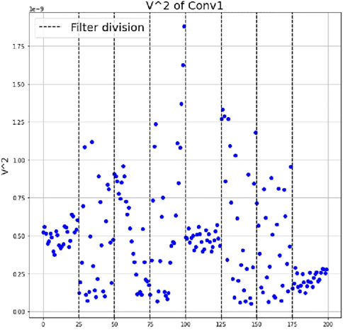
FIGURE 1. Temperature at equilibrium of the filters’ weights from the first convolutional layer, after training on MNIST. The vertical dashed lines divide one filter from the other. (See [1]).
The concept of temperature is necessarily an abstraction in the case of neural networks, but it leads to the analysis of the velocities of the weights and this allows to do interesting reasonings about the architecture, beyond the analogy. In the following, we exploit this theoretical framework to investigate the behaviour of the weights of the filters during and after the training.
2 Pruning experiment
In this section we describe our main experiment and we interpret it in the light of the treatment of our previous section.
2.1 The architecture
The architecture we use is quite simple and consists of 4 convolutional layers, separated by a dropout and a 2 × 2 max pooling layers (Figure 2).
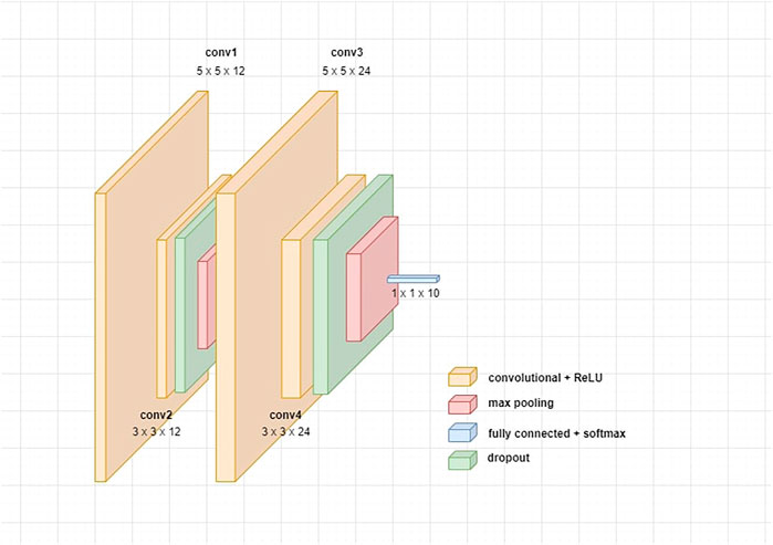
FIGURE 2. Architecture of our model.
Differently from [1, 10], we decide not to apply batch normalization to the ReLU activations of the convolutional layers, since it influences the distribution of the weights by normalizing them and we do not want this bias in our experiments. We optimize the network with SGD and, in particular, we use Adam optimizer with a starting learning rate of 0.001 and a dropout percentage of 0.1. We also make a comparison between trainings with a regularization decay of 0.001 and without it. Essentially, for both cases we draw the same conclusions on the dynamics of the weights: the only difference is due to the fact that the regularization confines the dynamics of the weights and lowers their velocities, with no considerable effects on performance.
We train this simple model on MNIST for 200 epochs, by maintaining the default split between train and test provided by Keras, and we consider the last 150 epochs as the equilibrium ones. As we can see from Figure 3, after 50 epochs accuracy and loss have reached their optimal values and continue slightly oscillating around them.
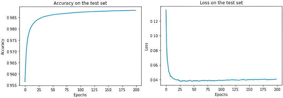
FIGURE 3. Accuracy and loss on the test set of MNIST, with regularization.
In Table 1, we show the final accuracy and loss on both the training and the test set, with or without regularization (accuracy and loss are obtained by averaging on 10 different trainings of the same model and computing standard deviation).
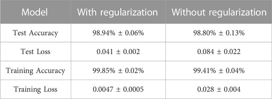
TABLE 1. Accuracy and loss on the test set with or without regularization.
We also train the same model on CIFAR10 with worse performance. This is due to the fact that CIFAR10 dataset is more heterogeneous than MNIST, hence our simple algorithm is not suitable for the more complex classification task. Then, we shall focus on the results obtained on MNIST; however, we will also make a comparison with the CIFAR10 experiments in Sec. 4, which confirm our findings.
2.2 Temperature-based pruning technique
The first experiment consists in looking at how the accuracy and the loss of the model get modified if we remove some filters, i.e., set their weights and biases equal to zero, depending on their temperature at equilibrium. We present the results obtained from the training on MNIST, in presence of regularization. To measure the equilibrium temperature of the filters, we take the squared velocities of the weights over the last 150 epochs and for each weight we compute the time average on the epochs. Then, for each filter, we compute the mean on the total number of weights of those average velocities. Instead of focusing on the time steps inside the last epoch of training, as in [1], we think that it is more representative to work between equilibrium epochs. Indeed, due to the SGD mechanism, the evolution of the velocities between time steps could be influenced by the fact we are looking at a different batch of data at each step. In Figure 4, we show the distribution of temperature for the 12 filters of the first convolutional layer, resulting from one of the 10 trainings. The distribution of hot and cold filters changes from training to training but it is qualitatively the same.
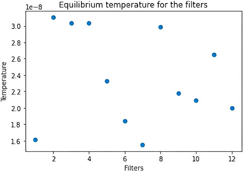
FIGURE 4. Distribution of the filters’ equilibrium temperature for the first layer, after training with regularization on MNIST. This is the result for one of the 10 trainings.
We now proceed with a description of our experiment, whose results are summarized in Table 2. If we set to zero the weights and biases of the two “hottest” filters, we get small variations of accuracy and loss, which respectively become 96.87% ± 2.77% and 0.12 ± 0.12. If, instead, we set to zero the parameters of the two “coldest” filters, accuracy and loss become respectively 75.70% ± 11.44% and 2.00 ± 1.01. We conclude that the removal of the two “coldest” filters leads to a bad performance, while removing the two “hottest” ones does not cause a significant drop in the accuracy.
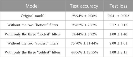
TABLE 2. Accuracy and loss on the test set after cropping different filters from the first CNN on MNIST, in case of regularization. Average and standard deviation are computed for 10 trainings.
We now perform a different experiment: we remove all the filters except the three “hottest” ones. We obtain that the performance of the model gets drastically worse: the accuracy is 24.44% ± 8.72% while the loss is 4.00 ± 1.40. Then, we also look at the metrics after removing all the filters except for the three “coldest” ones. The accuracy becomes 44.06% ± 18.55% and the loss becomes 4.00 ± 2.15. In this case, the performance of the model gets clearly worse since we are evaluating a model with only 3 filters in the first layer, but it is generally better than the one resulting from the evaluation of the model with only the three “hottest” ones, thus reinforcing the conclusions from our previous experiment.
In Table 2, we present the performance of the model, removing filters depending on their temperature.
We then repeated our experiments without regularization, obtaining the Table 3.
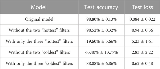
TABLE 3. Accuracy and loss on the test set after cropping different filters from the first CNN on MNIST, in absence of regularization.
We discover that “cold” filters have now an even greater role in the performance of the model, as “hot” filters, on the other hand, are of negligible importance. Hence, in absence of regularization, we have a more marked distinction between “cold” and “hot” filters, than in the regularization case. We will further discuss this difference and its interpretation in our next section.
It is interesting to compare our pruning technique to the one proposed in [16]. The authors in [16] prune filters depending on the sum of the absolute kernel weights, i.e., their l1-norm. The filters with the smallest norms are pruned, together with the resulting feature maps and with the filters in the next convolutional layer corresponding to those feature maps. This pruning technique is based on the fact that the smaller is the sum of the absolute values of the weights, the weaker are their activations compared to the other filters in that layer. All convolutional layers of the architecture are pruned by directly eliminating the weights of the filters with the smallest norms and then the model is retrained. The final performance after retraining the pruned model is better with respect to the initial one before pruning. Differently from them, we stress that we evaluate the performance of the model after pruning but we do not further train the pruned model to obtain the initial performance back. Indeed, by now, our study simply wanted to attest the validity of our reasoning about temperature as a pruning criterion, but next step is to effectively eliminate the pruned filters from every layer of the architecture and try both further training the model and training it from scratch without the pruned filters. What is more, as we will largely show in the next Section, “cold” filters are generally characterized by smaller l1-norm with respect to “hot” filters and they are precisely the ones we maintain and do not prune away. This is a major difference with the work in [16] and it is worth to further investigate it in the future. By now, we possibly link this difference to the fact that we are working on a much simpler architecture. However, our two pruning methods both follow from the observation of a disparity among the filters of the same CNN, either in the magnitude or in the temperature.
3 Analysis of the dynamics
In this section, we provide some insight into the result described in the previous section by linking the temperature of the filters to the dynamics of their weights. We first examine the trajectories of the weights and the behaviour of their velocities, then we establish a parallel of our findings with the work [10], as described in the first section.
3.1 Trajectories of the weights
In Figure 5, we show the trajectory for the 25 weights of the “coldest” and “hottest” filters of the first convolutional layer, for one of the trainings with regularization. Due to the presence of the regularization decay, which is the same for each filter, the weights remain stable along the epochs. However, if we look at the behaviour of their velocities at equilibrium (Figure 6), we notice that the weights vary from epoch to epoch in a noisy way and this is linked to the stochasticity of the training. In particular, differently from the “coldest” filter, we see that the “hottest” filter shows quite a large oscillation behaviour just after equilibrium is reached, which does not allow it to converge to a stable pattern soon. This means that the “hottest” filter employs more time to stabilize its weights to low velocities and, even when the metrics of the model have reached equilibrium, its weights continue to vary considerably. This is a way to see in which sense “hotter” filters influence less the total performance of the model: even when their weights highly oscillate, loss and accuracy remain stable around their equilibrium values and seem not being affected by that oscillation. This suggests that the 12 filters are not all necessary to the learning and this is confirmed in fact by our temperature pruning based experiments: the removal of the “hottest” filters will not produce a significant change in accuracy and loss.
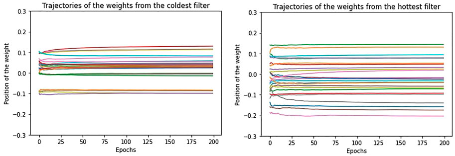
FIGURE 5. The trajectory of the weights from the “coldest” (on the left) and the “hottest” (on the right) filters in case of regularization.
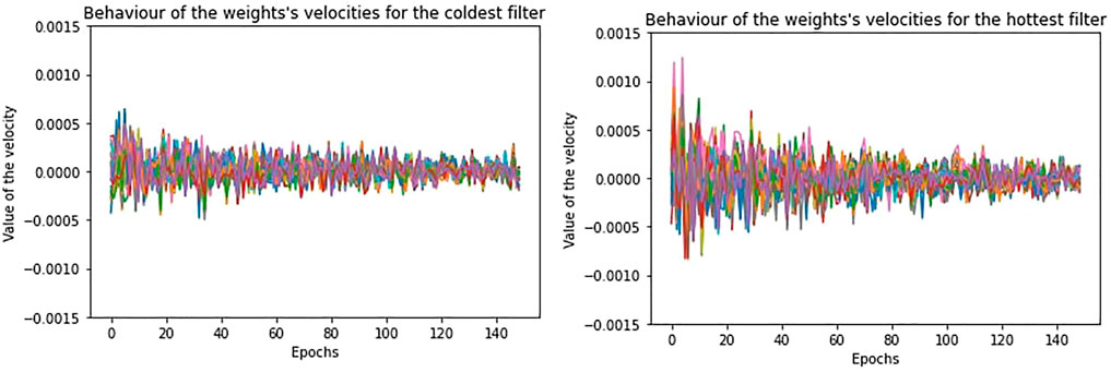
FIGURE 6. The behaviour at equilibrium for the velocities of the “coldest” (on the left) and “hottest” (on the right) filters, in case of regularization.
We discover that high temperature, which means high mean squared velocity, is not simply associated to a drift preventing weights from stabilizing, but it is also linked to a larger oscillation of the weights around their stable configuration. The dynamics of the weights is indeed characterized by two components: a drift and an oscillation, remembering the double component potential introduced in [10] we recalled in Sec. 1. However, in case of regularization, since the velocities are very low, the oscillation is very small.
If we repeat the same study on a training without regularization, the movement of the weights is less confined and shows greater oscillation, but we encounter the same relation between temperature and performance, as for the regularization case. In Figure 7 and Figure 8, we show the trajectories and velocities of the weights from the “coldest” and “hottest” filters of the first layer. As a consequence of what we have just said, without regularization, the temperature for the filters is generally higher and, differently from Figure 4, its distribution covers a larger range (Figure 9).
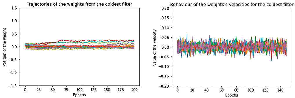
FIGURE 7. The trajectory of the weights and the behaviour of the velocities at equilibrium from the “coldest” filter, in absence of regularization.
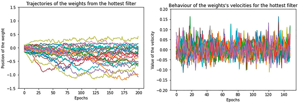
FIGURE 8. The trajectory of the weights and the behaviour of the velocities at equilibrium from the “hottest” filter, in absence of regularization.
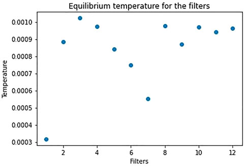
FIGURE 9. Distribution of the filters’ equilibrium temperature for the first layer, after training without regularization on MNIST. This distribution comes from one of the 10 trainings.
Indeed, with respect to the regularization case, now the filters differ much more in the trajectories of their weights. Some filters stabilize and reach low equilibrium temperature, even if higher with respect to the “cold” filters of the regularization case, while the others maintain high temperature, since most weights continue to diffuse or highly oscillate. What is more, since there is no regularization decay, the velocities of the weights do not exponentially decay along the equilibrium epochs as in Figure 6, but they remain the same.
3.2 Pattern of filters
We now look at the pattern learnt by the filters by simply printing their values at the last epoch. We can see that, in case of regularization, the filters are qualitative similar in the sense that they share a similar pattern, which is a mix of colours (Figure 10). This is due to the confinement of the dynamics. On the contrary, in absence of regularization, some filters are characterized by a clear contrast in colour, while others exhibit a mixed pattern (Figure 11). Without regularization, the difference between the filters is more pronounced; since the weights are not confined, the filters are free to reach different final configurations. Indeed, with respect to the regularization case, each filter covers a different range of values for the weights. As a consequence, we see an higher difference in temperature among the filters. Moreover, the three “coldest” filters contribute more to the performance of the model with respect to the three “coldest” of the regularized training (Tables 2, 3). With regularization, indeed, the weights can not move as much and the temperature of the filters is restricted to a smaller range. Hence, the weights necessary to optimally learn are distributed among a greater number of “cold” filters.
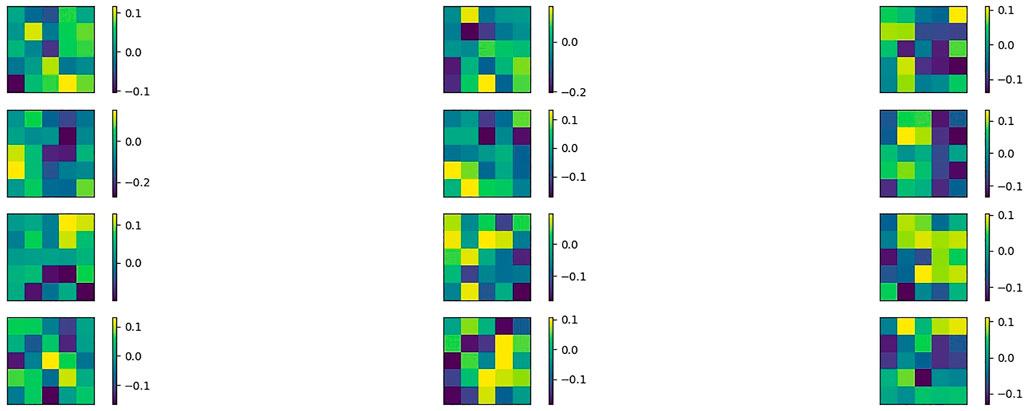
FIGURE 10. The patterns of the filters from the first convolutional layer on MNIST, in presence of regularization.
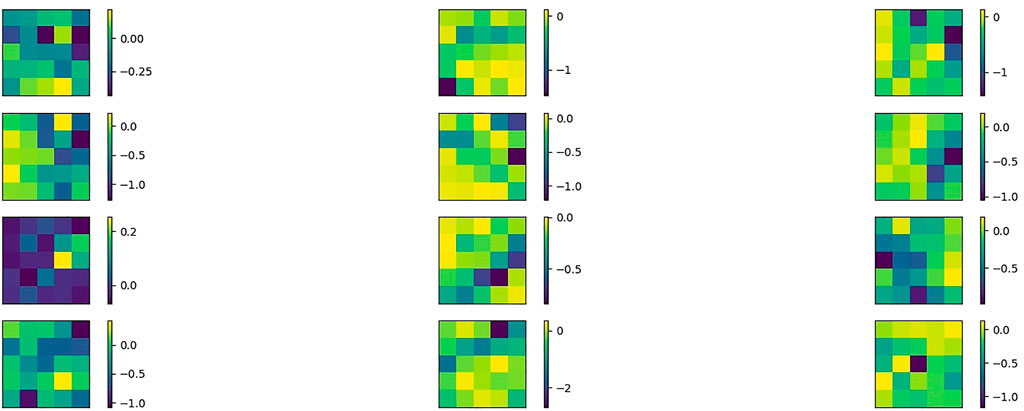
FIGURE 11. The patterns of the filters from the first convolutional layer on MNIST, in absence of regularization.
However, our general conclusions apply to both cases, with and without regularization. Cold filters reach their stable configuration and those are useful to the classification tasks, as our Tables 2, 3 show. Hot filters either are still moving or show a more oscillating behaviour, hence they do not reach a stable configuration when instead the macroscopic quantities of accuracy and loss do: those are the filters that can be safely removed without changing the accuracy of our model.
Overall, this study shows that, given the dataset and the model, only a certain number of filters per layer is really necessary to the learning process. Then, we can treat the number of filters as an hyperparameter of the model and we can use the temperature as a criterion to decide what is the minimum number of filters needed for the classification task.
3.3 The two components of the dynamics
As we briefly stated in the last section, we discover that the dynamics of the weights is characterized by two components, one takes into account the drift or translation and the other one the oscillation. In accordance with the introduction of a two terms potential by Chaudhari and Soatto in [10], we could link the component of the dynamics describing the translation (or drift) to the minimization of the “energetic” term of the potential, while the other component captures the noisy movement due to the “entropic” term. We stress again that the noisy movement is due to the stochasticity of the descent.
We study the dynamics of the weights by computing their mean squared displacement in time.
For each shift of epochs, we measure how much each weight has displaced in average from its initial position. We compute the MSD (mean square displacement) for the weights of each filter separately and we concentrate on the last 150 equilibrium epochs. As in [10], we would initially expect that, when convergence is reached, because of the noisy oscillations, the weights are characterized by Brownian motion around their stable position. However, we find out that, even at equilibrium, the weights are characterized by a slow drift.
In the theory of Brownian motion, the MSD is linked to time through the following expression:
where d is the dimensionality of the system and D is the diffusion constant. In our case, the dimensionality of the system is just 1, since every weight can be seen as a random walk in 1 dimension. In the case of Brownian motion, the mean squared displacement is linearly proportional to time and this is valid asymptotically, while at the beginning of the dynamics the relation is quadratic. In our case, the random walk is not a simple random walk, since the displacement at each step is not necessarily unitary and there is no equal probability to go in a direction or in the other. The dynamics of the weights is indeed subject to the minimization of a potential depending on all the other weights and, at every step of training, the update of the weight also depends on where it is located in the parameters’ space. Nevertheless, the same relation links the MSD to time and we have a different diffusion constant for each weight.
In Figure 12, we show the log plot of the mean squared displacement for the 25 weights of a filter of the first layer, in case of regularization. We also show the log plot of the mean displacement as an additional study of the dynamics of the weights. To better observe the behaviour of the displacement in time, we superimpose a linear and a quadratic trends in dashed black lines. We can see that, for large shifts in time, log (MSD) and log (epochs) are connected by a quadratic relation, that is, the mean squared displacement is quadratic in time. Accordingly, we can see that the mean displacement is linear in time. The oscillatory behaviour of the curve for some of the weights arises when the weight displaces only of a small quantity along the 150 epochs.
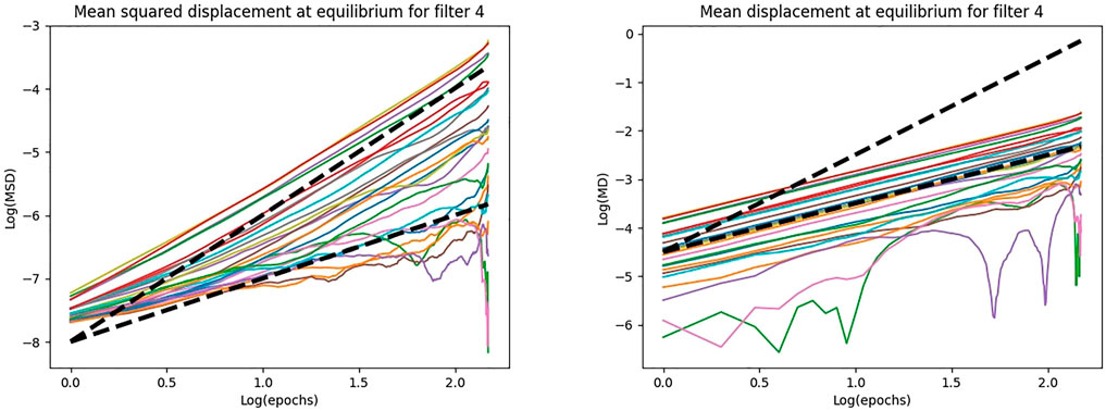
FIGURE 12. The log plot of the MSD and MD as function of the epochs for a filter of the first layer, in case of training with regularization on MNIST.
Then, at equilibrium, the weights do not exhibit pure Brownian motion, but they are characterized by a drift and this occurs for both “cold” and “hot” filters. Indeed, the linearity in time of the mean displacement indicates a translational dynamics. However, this drift is small and it is not detectable by simply looking at the trajectory of the weights over the epochs (Figure 5).
Exactly as Chaudhari and Soatto claim in [10], it seems that, at equilibrium, the weights do not simply move noisily around the final stable configuration, but their dynamics has a deterministic component that makes them move in a certain direction. However, differently from [10], we are not modeling the overall dynamics of all the weights of the network, but we concentrate only on the study of the weights of each filter.
Obviously, the drift occurs in a noisy way, since the descent is stochastic and the weights oscillate. If we discard the drift and only observe the mean squared displacement due to the noisy component of the dynamics, we discover that it is linear in time as for Brownian motion. In Figure 13, we show the MSD after subtracting the square of the mean displacement due to the drift. The mean displacement due to the drift is computed as
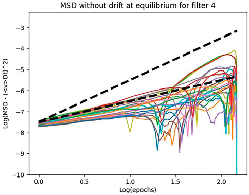
FIGURE 13. The log plot of the MSD due to only the noisy component of the dynamics.
The distinction between a drift and an oscillation component leads us to defining a new and more precise temperature for the filters, which is proportional to the mean kinetic energy due to only the noisy dynamics. We obtain the new mean kinetic energy by subtracting the mean of
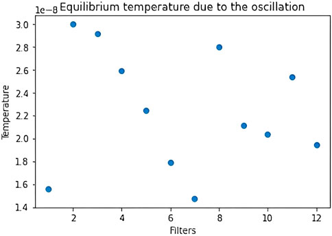
FIGURE 14. Distribution of the filters’ equilibrium temperature after subtracting the drift component from the dynamics. The filters are the ones of the first layer after training with regularization on MNIST and this distribution comes from one of the 10 trainings.
We obtain similar results on the training without regularization. In this case, the weights which reach a stable value have a very small drift, whereas the weights which do not stabilize show a larger drift. These findings confirm our pruning technique based on the temperature on the filters.
4 Results on CIFAR10
In this section we report some results on CIFAR10 dataset to validate our conclusions on the MNIST dataset. We train the model on CIFAR10 for 1000 epochs and we consider the last 700 as the equilibrium ones. We get essentially the same results as before for the dynamics of the weights of the filters. With regularization, the weights do not displace much from the initial position. At equilibrium, they slightly oscillate around their stable position and slowly drift. Without regularization, this also applies, but the oscillation is higher and some of the weights, usually from “hot” filters, diffuse to distant positions.
If we remove filters depending on their temperature, we obtain again that “hot” filters contribute less to the performance with respect to the “cold” ones (Tables 4, 5). However, with respect to the experiments on MNIST, in case of regularization the elimination of the “hot” filters causes now a considerable drop in the performance. This proves that all 12 filters are now necessary to the learning. This is reasonable, since the images in CIFAR10 show much more variety than those in MNIST, but we are training the same model on it. As described in the previous sections, regularization allows to maintain all filters more or less stable. If all filters are needed for the classification, regularization makes them all learning a pattern. Without regularization, instead, some filters (the “coldest”) learn a pattern, while others do not (the “hottest”). In fact, if we remove the “hottest” filters, the performance is nearly the same, as for MNIST.
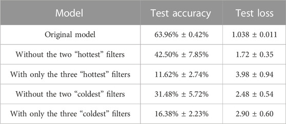
TABLE 4. Accuracy and loss on the test set after cropping different filters from the first CNN on CIFAR10, in case of regularization. Average and standard deviation are computed for 10 trainings.
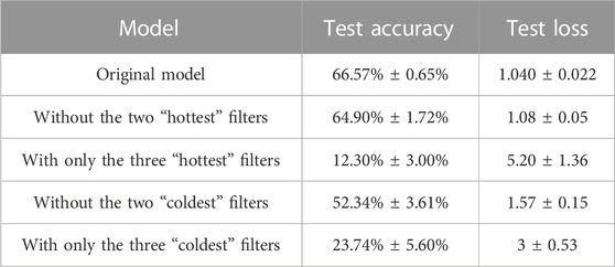
TABLE 5. Accuracy and loss on the test set after cropping different filters from the first CNN on CIFAR10, in absence of regularization.
5 Conclusion
We present a stringent thermodynamic analogy for SGD modeling in Deep Learning algorithms for classification tasks and a comparison with the literature. Our physically-guided understanding of neural networks allows us to present a temperature-based pruning technique on CNNs filters. Removing “hottest” filters does not significantly change the performance of the model, while removing “coldest” filters results in a significant drop in accuracy. Furthermore, for the future, we can also think of an additional training loop which supervises the temperature of the filters and stops optimizing the filters whose velocities do not decrease.
We show that physical reasoning based on thermodynamics, condensed matter physics and molecular dynamics can greatly improve our understanding of neural networks and allows us to propose new techniques, like temperature pruning filters, that we believe can improve the performance of machine learning algorithms.
Data availability statement
The original contributions presented in the study are included in the article/supplementary material, further inquiries can be directed to the corresponding author.
Author contributions
All authors listed have made a substantial, direct, and intellectual contribution to the work and approved it for publication.
Funding
This research was carried out under the grant COST Action CaLISTA, CA21109 and grant HE-MSCA-SE-2021-101086123-CaLIGOLA.
Acknowledgments
RF and ML would like to thank the DIFA at University of Bologna for the kind hospitality during the completion of this work.
Conflict of interest
The authors declare that the research was conducted in the absence of any commercial or financial relationships that could be construed as a potential conflict of interest.
Publisher’s note
All claims expressed in this article are solely those of the authors and do not necessarily represent those of their affiliated organizations, or those of the publisher, the editors and the reviewers. Any product that may be evaluated in this article, or claim that may be made by its manufacturer, is not guaranteed or endorsed by the publisher.
References
1. Fioresi R, Faglioni F, Morri F, Squadrani L. On the thermodynamic interpretation of deep learning systems. Geometric Science of Information: 5th International Conference (2021).
2. Krizhevsky A, Sutskever I, Hinton GE. Imagenet classification with deep convolutional neural networks. Adv Neural Inf Process Syst (2012) 25:1097–105.
3. LeCun Y, Bengio Y, Hinton G. Deep learning. nature (2015) 521(7553):436–44. doi:10.1038/nature14539
4. LeCun Y, Bottou L, Bengio Y, Haffner P. Gradient-based learning applied to document recognition. Proc IEEE (1998) 86(11):2278–324. doi:10.1109/5.726791
5. James Murdoch W, Singh C, Kumbier K, Abbasi-Asl R, Yu B. Interpretable machine learning: Definitions, methods, and applications. PNAS (2019) 116(44):22071–80. doi:10.1073/pnas.1900654116
6. Belle V, Papantonis I. Principles and practice of explainable machine learning. Front Big Data (2021) 4:688969. doi:10.3389/fdata.2021.688969
7. Jaynes ET. Information theory and statistical mechanics. Phys Rev (1957) 106(4):620–30. doi:10.1103/physrev.106.620
8. Hopfield J J Neurons with graded response have collective computational properties like those of two-state neurons. PNAS (1984) 81(10):3088–92. doi:10.1073/pnas.81.10.3088
9. Ackley DH, Hinton GE, TerrenceSejnowski J. A learning algorithm for Boltzmann machines. Cogn Sci (1985) 9(1):147–69. doi:10.1207/s15516709cog0901_7
10. Chaudhari P, Soatto S. Stochastic gradient descent performs variational inference, converges to limit cycles for deep networks. In: International Conference on Learning Representations ICLR 2018 (2018).
11. Chaudhari P, Anna C, Soatto S, LeCun Y, Baldassi C, Borgs C, et al. Entropy-sgd: Biasing gradient descent into wide valleys. J Stat Mech Theor Exp (2019) 2016.
12. Welling M, Yee W. Bayesian learning via stochastic gradient Langevin dynamics. In: International Conference on Machine Learning (2011).
13. Fioresi R, Chaudhari P, Soatto S. A geometric interpretation of stochastic gradient descent using diffusion metrics (2019).Entropy
14. Charles-Michel M. From tools in symplectic and Poisson geometry to j. m. souriau’s theories of statistical mechanics and thermodynamics. Entropy (2016) 18(10):370. doi:10.3390/e18100370
15. Anwar S, Hwang K, Sung W. Structured pruning of deep convolutional neural networks. ACM J Emerging Tech Comput Syst (2017) 13(3):1–18. doi:10.1145/3005348
16. Li H, Kadav A, Durdanovic I, Samet H, Graf HP. Pruning filters for efficient convnets. In: International Conference on Learning Representations ICLR 2017 (2017).
17. Li Q, Cheng T, Weinan E. Stochastic modified equations and adaptive stochastic gradient algorithms. In: Proceedings of the 34th International Conference on Machine Learning (2017).
18. Ma Y-A, Chen T, Emily B, Fox . A complete recipe for stochastic gradient mcmc. Neural Information Processing Systems (2015).
19. Baldassi C, Ingrosso A, Lucibello C, Saglietti L, Zecchina R. Subdominant dense clusters allow for simple learning and high computational performance in neural networks with discrete synapses. Phys Rev Lett (2015) 115:128101. doi:10.1103/physrevlett.115.128101
Keywords: deep learning, thermodynamics, machine learning, condensed matter physics, statistical mechanics, molecular dynamics
Citation: Lapenna M, Faglioni F and Fioresi R (2023) Thermodynamics modeling of deep learning systems for a temperature based filter pruning technique. Front. Phys. 11:1145156. doi: 10.3389/fphy.2023.1145156
Received: 15 January 2023; Accepted: 02 May 2023;
Published: 17 May 2023.
Edited by:
Florio M. Ciaglia, Universidad Carlos III de Madrid de Madrid, SpainReviewed by:
Domenico Pomarico, University of Bari Aldo Moro, ItalyRoberto Cilli, University of Bari Aldo Moro, Italy
Copyright © 2023 Lapenna, Faglioni and Fioresi. This is an open-access article distributed under the terms of the Creative Commons Attribution License (CC BY). The use, distribution or reproduction in other forums is permitted, provided the original author(s) and the copyright owner(s) are credited and that the original publication in this journal is cited, in accordance with accepted academic practice. No use, distribution or reproduction is permitted which does not comply with these terms.
*Correspondence: R. Fioresi, cml0YS5maW9yZXNpQHVuaWJvLml0