Interface transmittance and interface waves in acoustic Willis media

Acoustics Willis media, known as bianisotropic acoustic media, incorporate additional coupling between pressure and velocity and between momentum and volumetric strain in their constitutive equation. The extra coupling terms have a significant influence on acoustic wave behavior. In this paper, the unusual wave phenomena relevant to interfaces between homogeneous acoustic Willis media are theoretically studied. We show that Willis media offer more flexible control in wave front and energy flow when waves are transmitted through an interface. Different from traditional acoustic fluid, Willis acoustic media support edge and interface waves, for which the existence conditions and corresponding wave features are systematically investigated. The study unveils more possibilities for manipulating acoustic waves and may inspire new functional designs with acoustic Willis metamaterials.

1 Introduction

In the past 20 years, with the emergence and development of metamaterials, the design space of wave devices and other functionality structures has been enlarged unprecedentedly. Metamaterials often exhibit abnormal material properties that natural materials usually do not have, which can lead to many novel wave phenomena, such as negative refraction [1, 2], super lens [3, 4], and wave cloaking [5–7], providing broad application prospects and meanwhile appealing more sophisticated homogenization for the characterization of the dynamic effective properties. In this background, the theory of Willis materials, initially proposed by Willis [8] in the 1980s for the dynamic behavior of solid composite materials, has regained much attention [9–12].

Acoustic Willis media (known as acoustic bianisotropic media) incorporate coupling between pressure and velocity and between momentum and volumetric strain. It has been found that the local Willis coupling is directly related to the local asymmetry of unit cells [12]. Accordingly, different designs of acoustic Willis meta-atoms have been proposed, such as the membrane unit [13, 14], folded channel [15], and Helmholtz resonators [16, 17]. The extra degree of design freedom offered by the Willis coupling is utilized to realize various novel wave functionalities. Several studies have observed asymmetric reflection [11, 18–20] when waves are incident from different directions, based on which the unidirectional absorber may be realized [21–23]. When Willis meta-atoms are used in metasurfaces [13, 24–26] or metagratings [15, 27, 28] for anomalous refraction or reflections, independent and more efficient control of transmission and reflection can be realized. In addition, active mechanisms can be introduced to enhance the significance and flexibility of the coupling effect [29, 30], with which many non-reciprocal phenomena are demonstrated [30, 31]. Although remarkable progress has been made in recent years, most of the research on acoustic Willis coupling concentrates on the physical origin and design of Willis meta-atoms. Extended wave functionalities are usually demonstrated in reduced dimensionality, such as metasurfaces. Relatively, systematic theoretical study of wave behaviors in continuous Willis media has not received much attention. In recent works, some phenomena, such as sound scattering [32], sound focusing [33], and the topological phase transition [34] in Willis acoustic media, have been investigated.

In this paper, the unusual wave phenomena relevant to interfaces between homogeneous acoustic Willis media are theoretically studied. Section 2 discusses the general properties of bulk waves in Willis media, such as slowness curves, wave modes, and impedance. Section 3 explains the interface transmittance when a wave is incident into a Willis medium, which exhibits more flexible control in wave front and energy flow through material parameters. Section 4 considers the edge and interface waves in Willis media, partly demonstrated in [35]. Here, we present a more systematical examination considering other possibilities along with the corresponding parameter conditions and wave modes. Finally, conclusions are drawn in Section 5.

2 General bulk wave properties

Assuming harmonic motion with circular frequency ω and time convention $e^{-i\omega t}$, the momentum and continuity equations of Willis media are, respectively, as follows:

$\begin{array}{ccc}i\omega \mathbf{\mu }=\nabla p& \mathrm{a}\mathrm{n}\mathrm{d}& -i\omega \epsilon =\nabla \cdot \mathbf{v}\end{array},(1)$

where p is the acoustic pressure, ε the volumetric strain, v the particle velocity, and μ the momentum density. Distinct from traditional acoustic fluid, the constitutive relations of Willis media are characterized by

$\left\{\begin{array}{l}-p=\kappa \epsilon +\mathbf{S}\cdot \mathbf{v},\\ \mathbf{\mu }=\mathbf{\rho }\cdot \mathbf{v}+\mathbf{S}\epsilon ,\end{array}\right.(2)$

where κ and ρ are the bulk modulus and mass density, respectively. The density is in tensorial form and can be anisotropic. The vector S represents the acoustic Willis coupling term, whose fundamental physics originates from the locally monopolar–dipolar coupling and non-local phase effects of acoustic scatterers [12]. Here, we assume that the non-local effects could be ignored; hence, S is purely imaginary.

Combining Eqs 1, 2 gives the wave equation of Willis acoustic media:

${\left(\kappa -{\mathbf{S}}^{\mathrm{T}}{\mathbf{\rho }}^{-1}\mathbf{S}\right)}^{-1}\ddot{p}=\nabla \cdot \left(\left({\mathbf{\rho }}^{-1}+{\left(\kappa -{\mathbf{S}}^{\mathrm{T}}{\mathbf{\rho }}^{-1}\mathbf{S}\right)}^{-1}\left({\mathbf{\rho }}^{-1}\mathbf{S}\right)\otimes \left({\mathbf{\rho }}^{-1}\mathbf{S}\right)\right)\cdot \nabla p\right).(3)$

The wave equation is quite complex, and to simplify the analysis and highlight the Willis coupling effect, we consider in this section the isotropic density ρ, i.e., $\mathbf{\rho }=\rho \mathbf{I}$. According to [32], a dimensionless real vector $\mathbf{W}=i\mathbf{S}/\sqrt{\kappa \rho }$ is introduced for the Willis coupling for the sake of convenience. For a plane wave $p=\widehat{p}\exp \left(i\mathbf{k}\cdot \mathbf{r}\right)$ with $\widehat{p}$ and k being the complex amplitude and the wave vector, respectively, the dispersion equation is

$\left(1+W^2\right)k^2-{\left(\mathbf{W}\cdot \mathbf{k}\right)}^2=\frac{\rho }{\kappa }{\omega }^2,(4)$

where W = |W| and k = |k|. Eq. 4 has been formulated by [32]. In a two-dimensional (2D) case, the scenario of involved directions regarding the bulk wave propagation is depicted in Figure 1A, where ϕ is the azimuthal angle of W and ϕ′ is the angle between W and k.

FIGURE 1

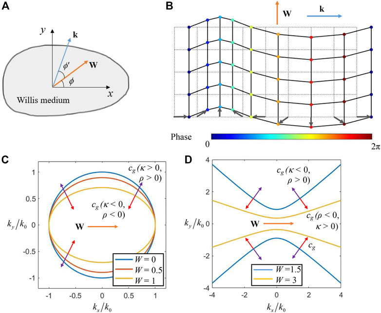
FIGURE 1. (A) Schematic representation of directions of the coupling vector and wave vector in the Willis acoustic medium. (B) Particle motion of a plane wave in the Willis acoustic medium. (C) Slowness curve of the positive or double negative Willis medium, $k_0=\omega \sqrt{\rho /\kappa }$. The purple arrows denote the group velocity of the medium with ρ > 0 and κ > 0, and the red arrows denote the group velocity of the medium with ρ < 0 and κ < 0. (D) Slowness curve of a single negative Willis medium, $k_0=\omega \sqrt{-\rho /\kappa }$. The red arrows denote the group velocity of the medium with ρ < 0 and κ > 0, and the purple arrows denote the group velocity of the medium with ρ > 0 and κ < 0.

Eq. 4 clearly shows that the slowness curve is an ellipse because of W. This is a natural consequence because the coupling vector brings directionality. Without loss of generality, align the x-axis with W, then Eq. 4 is simplified as

${k_x}^2+\left(1+W^2\right){k_y}^2=\frac{\rho }{\kappa }{\omega }^2.(5)$

Figure 1C shows the slowness curves of Willis media with different values of W. The major axis of the ellipse is collinear with the direction of W, and the ellipse tends to be flatter as W becomes larger. Compared with ordinary medium (W = 0), the phase velocity parallel to W remains unchanged, whereas the phase velocity perpendicular to W increases.

To further characterize the particle movements in Willis media, we investigate the velocity field of plane waves. Expressing the velocity field in the medium as $\mathbf{v}=\widehat{\mathbf{v}}\exp \left(i\mathbf{k}\cdot \mathbf{r}\right)$, the complex amplitude $\widehat{\mathbf{v}}$ can be derived as

$\widehat{\mathbf{v}}=\left(\begin{array}{l}{v}_{\parallel }\\ v_{\perp }\end{array}\right)=\frac{1}{\omega \rho }\left[k\left(\begin{array}{l}1\\ 0\end{array}\right)-\frac{W^2}{1+W^2}k\cos {\varphi }^{\prime }\left(\begin{array}{l}\cos {\varphi }^{\prime }\\ \sin {\varphi }^{\prime }\end{array}\right)-i\sqrt{\frac{\rho }{\kappa }}\omega \frac{W}{1+W^2}\left(\begin{array}{l}\cos {\varphi }^{\prime }\\ \sin {\varphi }^{\prime }\end{array}\right)\right]\widehat{p},(6)$

where the velocity components are decomposed in directions parallel to and perpendicular to the wave vector, represented by subscripts “$\parallel$” and “$\perp$,” respectively. Eq. 6 reveals that waves in the Willis acoustic medium are generally elliptically polarized, and because $\left|v_{\perp }\right|\ge \left|v_{\parallel }\right|$, the long axis of the ellipse is collinear with the wave vector direction. This is a typical feature different from the traditional acoustic media that only supports the longitudinal wave. A pure longitudinal wave ($v_{\perp }=0$) only happens when the coupling vector is collinear with the wave vector (${\varphi }^{\prime }=0\mathrm{o}\mathrm{r}\pi$). A typical wave picture is shown in Figure 1B, where the grid points of solid lines represent the real-time positions of particles, different colors represent their phases, and the dotted grid points represent their initial positions. For a wave propagating to the right, particles rotate clockwise around their equilibrium position in an elliptical orbit.

In the aforementioned discussion, ρ and κ are assumed to have positive values. As the Willis medium is often used to characterize metamaterials, it is reasonable to allow the negative values as well. If one of ρ and κ is negative, the definition of W should be modified as $\mathbf{W}=i\mathbf{S}/\sqrt{-\kappa \rho }$. As a result, Eq. 5 changes to

$k_x^2+\left(1-W^2\right)k_y^2=\frac{\rho }{\kappa }{\omega }^2.(7)$

In Eq. 7, if W ≤ 1, the medium does not support any traveling waves as no real solution of k exists. However, if W > 1, it is possible to find a real solution of k. In that case, the media have hyperbolic slowness curves, as shown in Figure 1D. The real axis of the hyperbola is perpendicular to W, and its eccentricity increases with W.

The group velocity can be determined by calculating the time-averaged intensity of power flow $\mathbf{I}=\mathrm{R}\mathrm{e}\left(p^{†}\mathbf{v}\right)/2$. For different sign combinations of ρ and κ, from Eqs 5, 7, respectively, they are expressed as

$\begin{array}{l}\left(\begin{array}{l}{I}_x\\ I_y\end{array}\right)=\frac{{\left|\widehat{p}\right|}^2}{2\omega \rho }\left(\begin{array}{c}\frac{k_x}{1+W^2}\\ k_y\end{array}\right),\mathrm{f}\mathrm{o}\mathrm{r}\left(\rho >0,\kappa >0\right)\mathrm{o}\mathrm{r}\left(\rho <0,\kappa <0\right),\\ \left(\begin{array}{l}{I}_x\\ I_y\end{array}\right)=\frac{{\left|\widehat{p}\right|}^2}{2\omega \rho }\left(\begin{array}{c}\frac{k_x}{1-W^2}\\ k_y\end{array}\right),\mathrm{f}\mathrm{o}\mathrm{r}\left(\rho >0,\kappa <0\right)\mathrm{o}\mathrm{r}\left(\rho <0,\kappa >0\right).\end{array}(8)$

The corresponding directions of group velocity are also plotted in Figures 1C,D for elliptic and hyperbolic slowness curves. For a medium with ρ < 0 and κ > 0, the group velocity points to the outer normal of the hyperbola, whereas for a medium with ρ > 0 and κ < 0, the group velocity points to the inner normal, as depicted in Figure 1D. If both ρ and κ are negative, Eq. 5 remains unchanged, so the slowness curve is elliptic. However, v changes in the opposite direction, as well as I. Hence, the group velocity points to the inner normal of the ellipse, as depicted in Figure 1C. The directions of group velocity can also be derived from the gradient of Eq. 5 or Eq. 7, but the causality constraint must be considered as in [36]. Further analysis shows that allowing the density to be anisotropic only changes the eccentricity of the ellipse or hyperbola (see Supplementary Material S1).

3 Interface transmittance and abnormal refraction

Having been acquainted with the wave properties, we consider in this section the transmittance of acoustic waves through the interface between an ordinary acoustic medium (Medium I) and a Willis medium (Medium II), as presented in Figure 2A. A plane wave is incident from the left side, and the incident, reflection, and refraction angles are θ_i, θ_r, and θ_t, respectively. The parameters on both sides are marked in the figure.

FIGURE 2

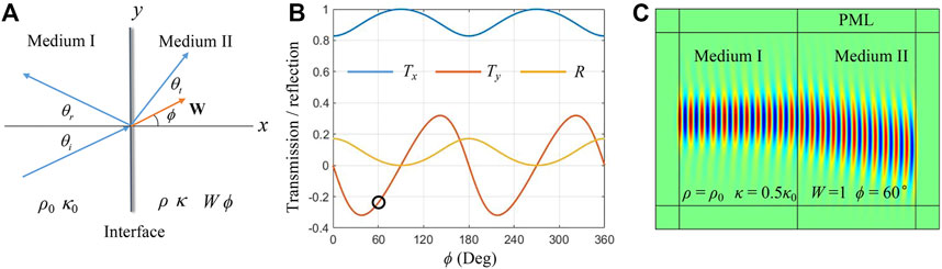
FIGURE 2. (A) Problem setup of the wave transmission across an interface between ordinary acoustic and Willis media. (B) Transmission and reflection power vary with ϕ for normal incidence. (C) FEM simulation of a normal incident Gaussian beam, corresponding to the dot in (B).

The reflected wave is on the side of the ordinary medium, and the reflection angle follows ${\theta }_r={\theta }_i$. On the other hand, the refraction angle in the Willis medium can be determined by the continuity of the tangential wave vector on the interface ($k^{\mathrm{I}\mathrm{I}}\sin {\theta }_t=k^{\mathrm{I}}\sin {\theta }_i$) as well as Eq. 4, where k^I and k^II are wave numbers on both sides, respectively. The refraction angle ${\theta }_t$ is ruled by

$\sqrt{\left(1+W^2-W^2(\cos ({\theta }_t-\varphi ){)}^2\right)}\sin {\theta }_i=\sqrt{\frac{{\kappa }_0\rho }{\kappa {\rho }_0}}\sin {\theta }_t.(9)$

As it is a transcendental equation, in general, θ_t can only be calculated numerically. However, for normal incidence (θ_i = 0), it is obvious that θ_t = 0, regardless of the magnitude and direction of the Willis coupling vector. In this case, the impedance of the Willis medium in the normal direction of the interface is $Z_n=p/v_{\parallel }$. Substituting Eq. 6 and noting that ϕ′ = ϕ, we get

$Z_n=\pm \sqrt{\kappa \rho }\left(\sqrt{1+W^2{\sin }^2\varphi }\pm iW\cos \varphi \right).(10)$

Therein, “±” represents the different signs when propagating to the positive or negative direction of the x-axis. In comparison to traditional acoustic fluid, an extra factor $\left(\sqrt{1+W^2{\sin }^2\varphi }\pm iW\cos \varphi \right)$ is added to the impedance. As the absolute value of this factor is greater than 1, the presence of Willis coupling will always increase the impedance, regardless of its azimuthal angle. The impedance matching condition at the interface is

$\begin{array}{ccc}\sqrt{{\kappa }_0{\rho }_0}=\sqrt{\kappa \rho \left(1+W^2\right)}& \mathrm{a}\mathrm{n}\mathrm{d}& \cos \varphi =0\end{array},(11)$

which indicates that the direction of the coupling vector must be perpendicular to the wave vector if the full transmission is required.

We learn in Section 2 that the direction of energy transmission may differ from the wave vector in the Willis medium. Even for the normal incidence, the energy flow direction may still deviate. Using Eq. 4, the reflection power ($R=\left|{\mathbf{I}}_r\right|/\left|{\mathbf{I}}_i\right|$) and the two components of the transmitted power flux ($T_x=I_{tx}/\left|{\mathbf{I}}_i\right|$; $T_y=I_{ty}/\left|{\mathbf{I}}_i\right|$) are calculated. Figure 2B presents the variation of transmission and reflection power versus the azimuthal angle ϕ under normal incidence. Other parameters are set as ρ = ρ₀, κ = 0.5κ₀ (ρ₀ = 1.2 kg/m³, κ₀ = 1.4 × 10⁵Pa, here and after), and W = 1 so that when ϕ = 90° or ϕ = 270°, the impedance matching conditions are satisfied. The calculated frequency is 7,000 Hz. Figure 2B shows that at these two points, the full transmission happens. When W points to other directions, there will be energy flow in the y direction and reflection. In Figure 2C, the deflected energy propagation for the case of Willis coupling with ϕ = 60° (as indicated by the dot in Figure 2B) is verified by finite element method (FEM) simulation considering the normal Gaussian beam incidence. All FEM simulations in this paper study are carried out via COMSOL software. The energy flux component in the y-direction corresponding to ϕ = 60° is negative. Correspondingly, it is observed that the wave beam deflects downward after passing through the interface.

For oblique incidence and considering negative parameters, more interesting phenomena can be obtained, as exemplified in Figure 3, wherein panels in the first row are the refractive patterns drawn from the slowness curve analysis, whereas the second row presents the results of FEM simulations of wave beams with 7,000 Hz. As shown in Figures 3A,D, we use a Willis medium with ρ > 0 and κ < 0, whereas in Figures 3B,E, we use a Willis medium with ρ < 0 and κ > 0. The used material parameters are given in Figures 3D,E. Because of the hyperbolic slowness curve, the wave number k_y of the incident wave cannot be less than a certain critical value to get a real wave number for the refraction wave, which is opposite to the case of positive parameters. Taking the 60° incident angle as an example, as indicated by the k_i arrow, the refractive k_r is determined from Figures 3A,B. The group velocity must have a positive x component to ensure energy always goes forward. For κ < 0 cases, as the group velocity points to the inner normal of the hyperbolic, negative refraction of phase velocity and positive refraction of group velocity are predicted, as shown in Figure 3A. Conversely, for the ρ < 0 case, as shown in Figure 3B, group velocity points to the outer normal of the hyperbolic. Thus, positive refraction of phase velocity and negative refraction of energy flow are predicted. From the FEM simulations in Figures 3D,E, the aforementioned analysis is confirmed by observing the refracted wave beam and wave front. As shown in Figures 3C,F, we use a Willis medium with ρ < 0 and κ < 0. The typical negative refraction is realized like the double ordinary doubly negative medium.

FIGURE 3

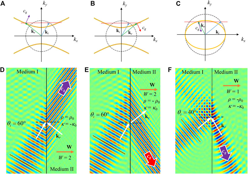
FIGURE 3. Interface refraction of Willis media with negative parameters. (A), (B), and (C) Slowness curves of the medium on the incident side (the gray dashed) and the refractive side (yellow solid). Blue and green arrows are the incident and refractive wave vectors, with equal tangential components indicated by the red dotted line. The red or purple arrows indicate the direction of group velocities. (D), (E), and (F) Corresponding FEM simulations of the cases of (A), (B), and (C), respectively, (pressure field).

4 Edge and interface waves

When boundary condition is considered in solving the wave equation, it is possible to find surface modes, for example, the well-known Rayleigh surface wave for solids. For an ordinary acoustic fluid, surface modes are not supported. However, in the realm of acoustic metamaterials, surface modes can be found in acoustic media with negative parameters [3, 37] or with gyrotropic mass [38]. In [35], we have partly demonstrated the existence of interface waves at the interface of two Willis media. Here, we present a more systematic examination of the edge and interface waves of Willis media.

4.1 Edge waves with sound hard boundary

As sketched in Figure 4A, we consider a semi-infinite of Willis acoustic medium, and the Cartesian coordinate system is established to make the open edge along the y-axis. Considering acoustic field explicitly expressed by $p=\widehat{p}\exp \left(i{k}_{x}x+i{k}_{y}y\right)$, for a possible edge mode, the field is traveling along the y-direction and attenuated away from the surface. Thus, k_y must be real, and k_x must have a positive (negative) imaginary part when the surface is on the left (right).

FIGURE 4

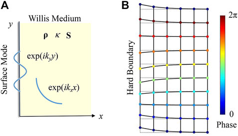
FIGURE 4. (A) Schematic representation of the surface mode of a semi-infinite Willis medium. (B) Typical wave pattern of edge mode for Willis acoustic media with isotropic density.

For sound soft (free) boundary, the requisite boundary condition is p (x = 0) = 0, which holds only for $\widehat{p}$ = 0. Then, the velocity $\widehat{\mathbf{v}}$ vanishes at the same time, and it is concluded that no edge mode is supported on the sound soft boundary. For sound hard boundary, it is required that the normal velocity on the boundary vanishes, that is, v_x (x = 0) = 0. Combining the boundary condition and the requirements of the wave vectors, we can conclude that surface waves may exist on the hard boundaries, and the parameter conditions for their existence are (Supplementary Material S2)

$\begin{array}{l}\frac{{\rho }_{yy}}{\kappa }>0\mathrm{a}\mathrm{n}\mathrm{d}i\left(S_x{\rho }_{yy}-S_y{\rho }_{xy}\right)>0,\mathrm{w}\mathrm{h}\mathrm{e}\mathrm{n}\mathrm{t}\mathrm{h}\mathrm{e}\mathrm{s}\mathrm{u}\mathrm{r}\mathrm{f}\mathrm{a}\mathrm{c}\mathrm{e}\mathrm{i}\mathrm{s}\mathrm{o}\mathrm{n}\mathrm{t}\mathrm{h}\mathrm{e}\mathrm{l}\mathrm{e}\mathrm{f}\mathrm{t},\\ \frac{{\rho }_{yy}}{\kappa }>0\mathrm{a}\mathrm{n}\mathrm{d}i\left(S_x{\rho }_{yy}-S_y{\rho }_{xy}\right)<0,\mathrm{w}\mathrm{h}\mathrm{e}\mathrm{n}\mathrm{t}\mathrm{h}\mathrm{e}\mathrm{s}\mathrm{u}\mathrm{r}\mathrm{f}\mathrm{a}\mathrm{c}\mathrm{e}\mathrm{i}\mathrm{s}\mathrm{o}\mathrm{n}\mathrm{t}\mathrm{h}\mathrm{e}\mathrm{r}\mathrm{i}\mathrm{g}\mathrm{h}\mathrm{t}.\end{array}(12)$

The wave number along the surface is $k_y=\pm \omega \sqrt{{\rho }_{yy}/\kappa }$. For the case of isotropic density and ρ > 0, κ > 0, the aforementioned condition reduces to be simply

$\begin{array}{l}{W}_x>0,\mathrm{w}\mathrm{h}\mathrm{e}\mathrm{n}\mathrm{t}\mathrm{h}\mathrm{e}\mathrm{s}\mathrm{u}\mathrm{r}\mathrm{f}\mathrm{a}\mathrm{c}\mathrm{e}\mathrm{i}\mathrm{s}\mathrm{o}\mathrm{n}\mathrm{t}\mathrm{h}\mathrm{e}\mathrm{l}\mathrm{e}\mathrm{f}\mathrm{t},\\ W_x<0,\mathrm{w}\mathrm{h}\mathrm{e}\mathrm{n}\mathrm{t}\mathrm{h}\mathrm{e}\mathrm{s}\mathrm{u}\mathrm{r}\mathrm{f}\mathrm{a}\mathrm{c}\mathrm{e}\mathrm{i}\mathrm{s}\mathrm{o}\mathrm{n}\mathrm{t}\mathrm{h}\mathrm{e}\mathrm{r}\mathrm{i}\mathrm{g}\mathrm{h}\mathrm{t}.\end{array}(13)$

Eq. 13 has an obvious geometric meaning that the vector W has to point away from the edge to find the edge wave. In this case, the wave mode can be analytically expressed as

$\begin{array}{l}p=\widehat{p}\exp \left(i{k}_{x}x+i{k}_{y}y\right),\\ v_y=\left[\pm \frac{1}{\sqrt{\kappa \rho }\left(1+W_y^2\right)}-\frac{i{W}_y}{\sqrt{\kappa \rho }\left(1+W_y^2\right)}\right]\widehat{p}\exp \left(i{k}_{x}x+i{k}_{y}y\right),\\ k_x=\pm \frac{W_x{W}_y}{\left(1+W_y^2\right)}\omega \sqrt{\rho /\kappa }+\frac{i{W}_x}{\left(1+W_y^2\right)}\omega \sqrt{\rho /\kappa },k_y=\pm \omega \sqrt{\rho /\kappa }.\end{array}(14)$

In Eq. 14, k_x is purely imaginary only when W is perpendicular to the boundary (W_y = 0), and the wave is exponentially attenuated away from the boundary. In other cases, k_x has both real and imaginary parts, which means that the edge wave is oscillatory attenuated away from the boundary (see Supplementary Material S3). In addition, non-zero W_y will make the imaginary part of k_x smaller. Hence, the attenuation will slow down further. It is also noticed that, unlike the bulk wave, the edge wave is linearly polarized, and particle velocity possesses only components along the interface. The wave pattern of the edge mode is shown in Figure 4B. The grid points on the solid lines represent the real-time position of particles, and the colors represent their phases. The dotted lines represent their initial positions.

FEM simulations are performed to verify the surface wave on the hard boundaries, as shown in Figure 5. Material parameters of the Willis medium are ρ = ρ₀, κ = κ₀, and W = 1. Two directions of the coupling vector, ϕ = 0° (Figure 5A) and ϕ = 180° (Figure 5B), are used here. The calculated frequency is 5,000 Hz. A pair of point sources with a half wavelength distance and opposite phases is set on the hard boundary to form a dipole, which can stimulate the surface mode more efficiently. In Figure 5A, the condition that W points away from the surface is satisfied. Correspondingly, the edge wave is observed along the y-axis. When W points to the surface, as in Figure 5B, no surface mode exists, and only the bulk mode is excited. Figure 5A shows that, for large W perpendicular to the edge, the wave vectors of edge mode and bulk mode differ much, so they are not easily coupled with each other. For edge waveguides having corners not so sharp, the edge wave can pass through without obvious scattering into the bulk, showing some robustness, as depicted in Figure 5C.

FIGURE 5

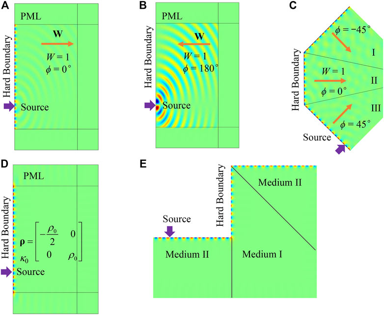
FIGURE 5. FEM simulations of surface waves on hard boundaries of Willis media (pressure field). (A) W points away from the surface. (B) W points to the surface. (C) Waveguide for the edge wave with possible leaking into bulk. (D) Edge wave without bulk leaking using an anisotropic density. (E) Robust edge waveguide with sharper corners using an anisotropic density.

To design a waveguide with more robustness, we can utilize a medium supporting edge wave that does not allow bulk waves. A simple choice is to use a single negative medium with isotropic density. However, such a medium does not possess edge mode because Eq. 12 cannot be satisfied, so we seek the possibility in the Willis medium with anisotropic density. The derived condition for the Willis medium that does not support bulk waves is (see Supplementary Material S4)

$\begin{array}{l}\frac{\kappa }{S_y^2{\rho }_{xx}-2S_x{S}_y{\rho }_{xy}+S_x^2{\rho }_{yy}+\kappa \left({\rho }_{xy}^2-{\rho }_{xx}{\rho }_{yy}\right)}<0\mathrm{a}\mathrm{n}\mathrm{d}\\ \left({\rho }_{xx}{\rho }_{yy}-{\rho }_{xy}^2\right)\left(S_y^2+S_x^2-\kappa {\rho }_{xx}-\kappa {\rho }_{yy}\right)>0.\end{array}(15)$

If a set of material parameters can satisfy Eq. 12 and 15 at the same time, the edge wave transmission would be very stable. In the example in Figure 5D, we choose a set of parameters as ρ_xx = – ρ₀/2, ρ_yy = ρ₀, ρ_xy = 0, κ = κ₀, $S_x=-i\sqrt{{\kappa }_0{\rho }_0}$, and S_y = 0 so that Eqs 12, 15 are simultaneously met for the edge on the left. All energy is concentrated at the boundary without any bulk waves. Moreover, in this exclusively edge-mode medium, a single monopole source is enough to excite the edge wave without matching its mode. In Figure 5E, a waveguide containing corners with the right angle is established using two different Willis media to meet the corresponding parameter requirements on the boundary of different orientations. Therein, Medium I is the same as that in Figure 5D, and Medium II is simply obtained by rotation from Medium I. The edge wave transmits through the designed route without energy leaking into the bulk.

4.2 Interface waves between two media

In practice, if the impedance of the Willis and adjacent media significantly differs, their interface can be treated as an ideal soft or hard boundary. For other cases, further analysis is required to estimate whether interface modes exist.

Consider the problem shown in Figure 6A. The ordinary acoustic medium (Medium I) on the left side and the Willis medium (Medium II) on the right side form an interface along the y-axis. In order to simplify the problem, the discussion is limited to Willis media with isotropic density and ρ > 0, κ > 0. The density and bulk modulus of the ordinary medium are ρ₀ and κ₀, respectively. The parameters of the Willis medium are ρ, κ, and W. For an interface wave, the pressure fields on the two sides can be written as $p^{\mathrm{I}}=\widehat{p}\exp \left(i{k}_x^{\mathrm{I}}x+i{k}_{s}y\right)$ and $p^{\mathrm{I}\mathrm{I}}=\widehat{p}\exp \left(i{k}_x^{\mathrm{I}\mathrm{I}}x+i{k}_{s}y\right)$, respectively, where k_s is the tangential wave vector along the interface. It must be continuous and real on both sides. $k_x^{\mathrm{I}}$ and $k_x^{\mathrm{I}\mathrm{I}}$ are normal wave vectors, which should satisfy $\mathrm{I}\mathrm{m}\left(k_x^{\mathrm{I}}\right)<0$ and $\mathrm{I}\mathrm{m}\left(k_x^{\mathrm{I}\mathrm{I}}\right)>0$ to ensure attenuation in the direction away from the interface. The conditions for the existence of interfacial waves are as follows (see Supplementary Material S5):

$W_x>0,\frac{\overline{\rho }}{\overline{\kappa }}>1,\frac{W_x^2}{{\overline{\kappa }}^2}+\frac{\overline{\rho }}{\overline{\kappa }}\left(1+W^2\right)>{\left(\frac{\overline{\rho }}{\overline{\kappa }}\right)}^2\left(1+W^2\right)\left(1+W_y^2\right),(16)$

where $\overline{\rho }=\rho /{\rho }_0$ and $\overline{\kappa }=\kappa /{\kappa }_0$. The interface mode is difficult to be expressed analytically, so we demonstrate it with a specific numerical example in Figure 6B. The parameters are set as $\overline{\rho }=0.2,\overline{\kappa }=0.1$, W = 1, and ϕ = 0°. The grid points in Figure 6B represent the real-time positions of the particle. Due to the non-zero normal velocity, particles near the interface rotate in an elliptical trajectory around their equilibrium positions, which is very different from the edge mode. At the interface, only the normal velocity maintains continuity. The two media have a relative slip in the tangential direction. The FEM simulation of the interface wave is shown in Figure 7A with the same parameters. The influence of the material parameters on the robustness of interface waves is analyzed in Supplementary Materials S6.

FIGURE 6

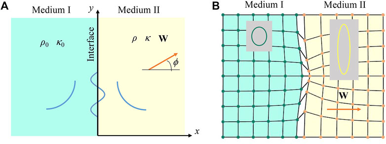
FIGURE 6. (A) Schematic representation of the interface mode between an ordinary medium (Medium I) and a Willis medium (Medium II). The interface mode is a traveling mode along the surface and evanescent away from the interface. (B) Wave mode of the interface wave, where the interface expands at a finite width to clearly display the particle motion on both sides. The insets show typical particle orbits on each side.

FIGURE 7

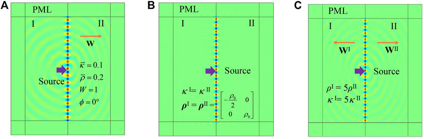
FIGURE 7. FEM simulations of interface waves (pressure field). (A) Medium I, an ordinary medium; Medium II, a Willis medium. (B) Both sides are Willis media with parameters that satisfy Eq. 17. (C) Both sides are Willis media with parameters that satisfy Eq. 18. In (A), (B), and (C), the sources are 5,000-Hz dipoles marked by arrows.

In the problem setup shown in Figure 6A, if the two domains are both Willis media, the analysis of the interface wave is more complex, so the general situation is not studied. However, if the two media meet some specific conditions, the problem will become intuitive. In Section 4.1, we use the boundary condition that the normal velocity is zero to derive the existence condition Eq. 12 for edge waves and the corresponding edge wave number $k_y=\pm \omega \sqrt{{\rho }_{yy}/\kappa }$. The derivation is reversible; that is, if $k_y=\pm \omega \sqrt{{\rho }_{yy}/\kappa }$ and Eq. 12 holds, the normal velocity on the boundary must be zero. Thus, we conclude that, in the current problem of two Willis domains, if the tangential wave numbers on both sides of the interface are the same and Eq. 12 holds for each side, the continuity condition of the interface will always be met. In this situation, the media on both sides are mutually sound hard boundaries to each other, so the interface wave can be supported. On the premise that ${\rho }_{yy}^{\mathrm{I}}/{\kappa }^{\mathrm{I}}={\rho }_{yy}^{\mathrm{I}\mathrm{I}}/{\kappa }^{\mathrm{I}\mathrm{I}}$, an existence condition for the interface wave reads

${\rho }_{yy}^{\mathrm{I}}/{\kappa }^{\mathrm{I}}={\rho }_{yy}^{\mathrm{I}\mathrm{I}}/{\kappa }^{\mathrm{I}\mathrm{I}}>0,i\left(S_x^{\mathrm{I}}{\rho }_{yy}^{\mathrm{I}}-S_y^{\mathrm{I}}{\rho }_{xy}^{\mathrm{I}}\right)<0,i\left(S_x^{\mathrm{I}\mathrm{I}}{\rho }_{yy}^{\mathrm{I}\mathrm{I}}-S_y^{\mathrm{I}\mathrm{I}}{\rho }_{xy}^{\mathrm{I}\mathrm{I}}\right)>0.(17)$

An FEM example is shown in Figure 7B. For convenience, the parameters of Medium II are obtained by the mirror symmetry operation of Medium I about the y-axis, so if Eq. 17 holds on one side, it also holds on the other side. The parameters are ρ^I = ρ^II (components are marked in Figure 7B), κ^I = κ^II = κ₀, $S_x^{\mathrm{I}}=i\sqrt{{\kappa }_0{\rho }_0}$, $S_x^{\mathrm{I}\mathrm{I}}=-i\sqrt{{\kappa }_0{\rho }_0}$, and $S_y^{\mathrm{I}}=S_y^{\mathrm{I}\mathrm{I}}=0$. Additionally, the parameters in Figure 7B satisfy Eq. 15, so a pure interface wave is excited without bulk leaking.

When the density is isotropic, ρ > 0, and κ > 0, Eq. 17 reduces to

${\rho }^{\mathrm{I}}/{\kappa }^{\mathrm{I}}={\rho }^{\mathrm{I}\mathrm{I}}/{\kappa }^{\mathrm{I}\mathrm{I}},W_x^{\mathrm{I}}<0,W_x^{\mathrm{I}\mathrm{I}}>0.(18)$

Similarly, Eq. 18 implies that vectors W on both sides point away from the interface. An example is shown in Figure 7C. The parameters in Medium I are ρ^I = 5ρ₀, κ^I = 5κ₀, W^I = 1, and ϕ^I = 180°, and those in Medium II are ρ^II = ρ₀, κ^II = κ₀, W^II = 1, and ϕ^II = 0°_. The density and bulk modulus of the Willis medium on the left side are both five times those on the right side, so the tangential wave vector is continuous on the interface. The coupling vector point away from the interface on both sides. An interface wave is observed as Eq. 18 is satisfied.

5 Conclusion

In this study, unusual wave phenomena relevant to interfaces in the homogeneous acoustic Willis media are studied theoretically. We show that the media exhibit anisotropic features due to the Willis coupling vector terms, and the slowness curve can be tuned between elliptical and hyperbolic shapes. The interface transmittance can be adjusted by the magnitude and direction of the coupling vector, which offers more flexible control in the compared with the traditional acoustic fluids. The Willis acoustic media support edge waves at acoustic hard boundaries and interface waves at interfaces between an ordinary acoustic fluid and a Willis medium or between two Willis media. Particularly, the edge modes may also exist in certain Willis media that do not support bulk modes, in which case they can achieve high transmission.

The study unveils more possibilities for manipulating acoustic waves and may inspire new functional designs with acoustic Willis metamaterials. It should be noted that this theoretical study assumes continuous acoustic media already with Willis coupling. On the experimental side, designing metamaterials with the wanted coupling effect is still an ongoing and challenging task. Especially for those wave phenomena calling for a strong S vector and negative density or modulus, the experimental demonstration may necessitate a more sophisticated design.

Data availability statement

The original contributions presented in the study are included in the article/Supplementary Material. Further inquiries can be directed to the corresponding author.

Author contributions

HQ wrote the original draft. XL and AZ reviewed and revised the manuscript. XL supervised the work. All authors contributed to the article and approved the submitted version.

Funding

This work was supported by the National Natural Science Foundation of China (Grant no. 11972080) and the Innovation Foundation of Maritime Defense Technologies Innovation Center (Grant no. JJ-2021-719-06). HQ acknowledges the support of the research start-up fund from Shijiazhuang Tiedao University.

Conflict of interest

The authors declare that the research was conducted in the absence of any commercial or financial relationships that could be construed as a potential conflict of interest.

Publisher’s note

All claims expressed in this article are solely those of the authors and do not necessarily represent those of their affiliated organizations, or those of the publisher, the editors, and the reviewers. Any product that may be evaluated in this article, or claim that may be made by its manufacturer, is not guaranteed or endorsed by the publisher.

Supplementary material

The Supplementary Material for this article can be found online at: https://www.frontiersin.org/articles/10.3389/fphy.2023.1141129/full#supplementary-material

References

1. Zhang XD, Liu ZY. Negative refraction of acoustic waves in two-dimensional phononic crystals. Appl Phys Lett (2004) 85:341–3. doi:10.1063/1.1772854

CrossRef Full Text | Google Scholar

2. Zhu R, Liu XN, Hu GK, Sun CT, Huang GL. Negative refraction of elastic waves at the deep-subwavelength scale in a single-phase metamaterial. Nat Commun (2014) 5:5510–8. doi:10.1038/ncomms6510

PubMed Abstract | CrossRef Full Text | Google Scholar

3. Ambati M, Fang N, Sun C, Zhang X. Surface resonant states and superlensing in acoustic metamaterials. Phys Rev B (2007) 75:195447. doi:10.1103/physrevb.75.195447

CrossRef Full Text | Google Scholar

4. Zhang HK, Zhou XM, Hu GK. Shape-adaptable hyperlens for acoustic magnifying imaging. Appl Phys Lett (2016) 109:224103. doi:10.1063/1.4971364

CrossRef Full Text | Google Scholar

5. Chen HY, Chan CT. Acoustic cloaking in three dimensions using acoustic metamaterials. Appl Phys Lett (2007) 91:183518. doi:10.1063/1.2803315

CrossRef Full Text | Google Scholar

6. Chen Y, Liu XN, Hu GK. Latticed pentamode acoustic cloak. Sci Rep (2015) 5:15745. doi:10.1038/srep15745

PubMed Abstract | CrossRef Full Text | Google Scholar

7. Zhang HK, Chen Y, Liu XN, Hu GK. An asymmetric elastic metamaterial model for elastic wave cloaking. J Mech Phys Sol (2020) 135:103796. doi:10.1016/j.jmps.2019.103796

CrossRef Full Text | Google Scholar

8. Willis JR. Variational principles for dynamic problems for inhomogeneous elastic media. Wave Motion (1981) 3:1–11. doi:10.1016/0165-2125(81)90008-1

CrossRef Full Text | Google Scholar

9. Milton GW, Briane M, Willis JR. On cloaking for elasticity and physical equations with a transformation invariant form. New J Phys (2006) 8:248. doi:10.1088/1367-2630/8/10/248

CrossRef Full Text | Google Scholar

10. Milton GW, Willis JR. On modifications of Newton's second law and linear continuum elastodynamics. P Roy Soc A (2007) 463:855–80. doi:10.1098/rspa.2006.1795

CrossRef Full Text | Google Scholar

11. Muhlestein MB, Sieck CF, Alu A, Haberman MR. Reciprocity, passivity and causality in Willis materials. P Roy Soc A (2016) 472:20160604. doi:10.1098/rspa.2016.0604

CrossRef Full Text | Google Scholar

12. Sieck F, Alù A, Haberman MR. Origins of Willis coupling and acoustic bianisotropy in acoustic metamaterials through source-driven homogenization. Phys Rev B (2017) 96:104303. doi:10.1103/physrevb.96.104303

CrossRef Full Text | Google Scholar

13. Koo S, Cho C, Jeong JH, Park N. Acoustic omni meta-atom for decoupled access to all octants of a wave parameter space. Nat Commun (2016) 7:13012. doi:10.1038/ncomms13012

PubMed Abstract | CrossRef Full Text | Google Scholar

14. Muhlestein MB, Sieck CF, Wilson PS, Haberman MR. Experimental evidence of Willis coupling in a one-dimensional effective material element. Nat Commun (2017) 8:15625. doi:10.1038/ncomms15625

PubMed Abstract | CrossRef Full Text | Google Scholar

15. Quan L, Ra'di Y, Sounas DL, Alu A. Maximum Willis coupling in acoustic scatterers. Phys Rev Lett (2018) 120:254301. doi:10.1103/physrevlett.120.254301

PubMed Abstract | CrossRef Full Text | Google Scholar

16. Melnikov A, Chiang YK, Quan L, Oberst S, Alù A, Marburg S, et al. Acoustic meta-atom with experimentally verified maximum Willis coupling. Nat Commun (2019) 10:3148. doi:10.1038/s41467-019-10915-5

PubMed Abstract | CrossRef Full Text | Google Scholar

17. Groby JP, Malléjac M, Merkel A, Romero-García V, Tournat V, Torrent D, et al. Analytical modeling of one-dimensional resonant asymmetric and reciprocal acoustic structures as Willis materials. New J Phys (2021) 23:053020. doi:10.1088/1367-2630/abfab0

CrossRef Full Text | Google Scholar

18. Liu Y, Liang Z, Zhu J, Xia L, Mondain-Monval O, Brunet T, et al. Willis metamaterial on a structured beam. Phys Rev X (2019) 9:011040. doi:10.1103/physrevx.9.011040

CrossRef Full Text | Google Scholar

19. Meng Y, Hao Y, Guenneau S, Wang S, Li J. Willis coupling in water waves. New J Phys (2021) 23:073004. doi:10.1088/1367-2630/ac0b7d

CrossRef Full Text | Google Scholar

20. Qu HF, Liu XN, Hu GK. Mass-spring model of elastic media with customizable Willis coupling. Int J Mech Sci (2022) 224:107325. doi:10.1016/j.ijmecsci.2022.107325

CrossRef Full Text | Google Scholar

21. Merkel A, Romero-García V, Groby JP, Li J, Christensen J. Unidirectional zero sonic reflection in passive PT-symmetric Willis media. Phys Rev B (2018) 98:201102. doi:10.1103/physrevb.98.201102

CrossRef Full Text | Google Scholar

22. Esfahlani H, Mazor Y, Alù A. Homogenization and design of acoustic Willis metasurfaces. Phys Rev B (2021) 103:054306. doi:10.1103/physrevb.103.054306

CrossRef Full Text | Google Scholar

23. Wiest T, Seepersad CC, Haberman MR. Robust design of an asymmetrically absorbing Willis acoustic metasurface subject to manufacturing-induced dimensional variations. J Acoust Soc Am (2022) 151:216–31. doi:10.1121/10.0009162

PubMed Abstract | CrossRef Full Text | Google Scholar

24. Díaz-Rubio A, Tretyakov SA. Acoustic metasurfaces for scattering-free anomalous reflection and refraction. Phys Rev B (2017) 96:125409. doi:10.1103/physrevb.96.125409

CrossRef Full Text | Google Scholar

25. Li J, Shen C, Diaz-Rubio A, Tretyakov SA, Cummer SA. Systematic design and experimental demonstration of bianisotropic metasurfaces for scattering-free manipulation of acoustic wavefronts. Nat Commun (2018) 9:1342. doi:10.1038/s41467-018-03778-9

PubMed Abstract | CrossRef Full Text | Google Scholar

26. Chen Y, Li X, Hu G, Haberman MR, Huang G. An active mechanical Willis meta-layer with asymmetric polarizabilities. Nat Commun (2020) 11:3681–8. doi:10.1038/s41467-020-17529-2

PubMed Abstract | CrossRef Full Text | Google Scholar

27. Craig SR, Su X, Norris A, Shi C. Experimental realization of acoustic bianisotropic gratings. Phys Rev Appl (2019) 11:061002. doi:10.1103/physrevapplied.11.061002

CrossRef Full Text | Google Scholar

28. Quan L, Yves S, Peng Y, Esfahlani H, Alù A. Odd Willis coupling induced by broken time-reversal symmetry. Nat Commun (2021) 12:2615–9. doi:10.1038/s41467-021-22745-5

PubMed Abstract | CrossRef Full Text | Google Scholar

29. Cho C, Wen X, Park N, Li J. Acoustic Willis meta-atom beyond the bounds of passivity and reciprocity. Commun Phys (2021) 4:82–8. doi:10.1038/s42005-021-00584-6

CrossRef Full Text | Google Scholar

30. Zhai Y, Kwon HS, Popa BI. Active Willis metamaterials for ultracompact nonreciprocal linear acoustic devices. Phys Rev B (2019) 99:220301. doi:10.1103/physrevb.99.220301

CrossRef Full Text | Google Scholar

31. Popa BI, Zhai Y, Kwon HS. Broadband sound barriers with bianisotropic metasurfaces. Nat Commun (2018) 9:5299. doi:10.1038/s41467-018-07809-3

PubMed Abstract | CrossRef Full Text | Google Scholar

32. Muhlestein MB, Goldsberry BM, Norris AN, Haberman MR. Acoustic scattering from a fluid cylinder with Willis constitutive properties. P Roy Soc A (2018) 474:20180571. doi:10.1098/rspa.2018.0571

CrossRef Full Text | Google Scholar

33. Lawrence AJ, Goldsberry BM, Wallen SP, Haberman MR. Numerical study of acoustic focusing using a bianisotropic acoustic lens. J Acoust Soc Am (2020) 148:EL365–9. doi:10.1121/10.0002137

PubMed Abstract | CrossRef Full Text | Google Scholar

34. Qu HF, Liu XN, Hu GK. Topological valley states in sonic crystals with Willis coupling. Appl Phys Lett (2021) 119:051903. doi:10.1063/5.0055789

CrossRef Full Text | Google Scholar

35. Li ZY, Qu HF, Zhang HK, Liu XN, Hu GK. Interfacial wave between acoustic media with Willis coupling. Wave Motion (2022) 112:102922. doi:10.1016/j.wavemoti.2022.102922

CrossRef Full Text | Google Scholar

36. Smith DR, Schurig D. Electromagnetic wave propagation in media with indefinite permittivity and permeability tensors. Phys Rev Lett (2003) 90:077405. doi:10.1103/physrevlett.90.077405

PubMed Abstract | CrossRef Full Text | Google Scholar

37. Bobrovnitskii YI. A Rayleigh-type wave at the plane interface of two homogeneous fluid half-spaces. Acoust Phys (2011) 57:595–7. doi:10.1134/s1063771011050046

CrossRef Full Text | Google Scholar

38. Zhou X, Zhao Y. Unusual one-way edge state in acoustic gyroscopic continuum. Sci China Phys Mech (2018) 62:14612–7. doi:10.1007/s11433-018-9268-9

CrossRef Full Text | Google Scholar