 Peng Dong1
 Zheng-Yi Ma
94% of researchers rate our articles as excellent or good
Learn more about the work of our research integrity team to safeguard the quality of each article we publish.
Find out more
ORIGINAL RESEARCH article
Front. Phys., 09 March 2023
Sec. Interdisciplinary Physics
Volume 11 - 2023 | https://doi.org/10.3389/fphy.2023.1137999
This article is part of the Research TopicNonlocal Integrable System and Nonlinear WavesView all 8 articles
The integrable Alice–Bob system with the shifted parity and delayed time reversal is presented through the Lax pair for the (1 + 1)-dimensional Boussinesq equation. After introducing an extended Bäcklund transformation, this system shows abundant exact solutions with the auxiliary functions consisting of hyperbolic functions or rational functions. The corresponding soliton structures contain line solitons, breathers, and lumps, all which satisfied the shifted parity and delayed time-reversal symmetry for the states of Alice A and Bob B. In particular, some lower-order circumstances can be expressed through their explicit solutions and their dynamic structures.
For one (1 + 1)-dimensional model, except for identity transformation, there are the shifted parity
with x0 and t0 being arbitrary constants [1, 2]. However, the Alice–Bob system, which can be successively used to describe two-place physical problems, may be entangled with each other through the following relation:
with the state of Alice A ≡ A(x, t) and the Bob’s state B ≡ B(x′, t′);
For an illustrated model, the (1 + 1)-dimensional Boussinesq equation has the following form:
or
where
and its adjoint version is as follows:
where I is an imaginary unit.
In non-linear science, this equation is one of the important prototypic models. It can be used to study the dynamics of thin inviscid layers with a free surface, the non-linear string, and the propagation of waves in elastic rods and in the continuum limit of lattice dynamics or coupled electrical circuits. Multiple complex soliton solutions through multiple exponential function schemes, interactions between solitons and cnoidal periodic waves using the truncated Painlevé expansion method, and soliton solutions by the extended Kudryashov’s approach can all be presented [8–10].
Except for the former works where the physical quantity
After adopting the
The corresponding Lax pairs of Eqs 5, 6areas follows:
with
and we can obtain the following coupled equations:
when σ = 0. After letting w = A+ B and v = A− B, the non-local systems (9) and (10) are a direct result from Eqs 14, 15.
Another method to derive the non-local systems (9) and (10) is the dark parameterization approach [14–17]. For the coupling Boussinesq system,
w0 is the usual solution of Eq. 3; when taking w = u + vα (α is a dark parameter) and n = 1, the coupled equations are as follows:
and
These equations can directly derive the non-local systems (9) and (10) through u = A+ B and v = A− B.
The rest of this paper is organized as follows: in Section 2, after introducing an extended Bäcklund transformation, the Hirota bilinear form is presented through an undetermined function f, which may contain some soliton solutions for the Alice–Bob systems (9) and (10) of the (1 + 1)-dimensional Boussinesq Eq. 3. Then, the hyperbolic function solution and the rational solution for this system are shown subsequently. In order to illustrate more clearly, three kinds of explicit solutions and their corresponding soliton structures are given for the lower-order circumstances. All of these results satisfy the symmetry of
We first introduce an extended Bäcklund transformation:
with b and c being two constants; f ≡ f (x, t) is an undetermined function and satisfies the following conditions:
By substituting Eq. 19 into the non-local systems (9) and (10), we obtain the following bilinear form:
where Hirota’s bilinear derivative operators
Eq. 21 also has the following explicit expression:
Through the bilinear form (21) or Eq. 23, the function f exists in the following form of the hyperbolic function for the Boussinesq Eq. 3 [4–6].
where {ν} = {νi = ±1} and ki(i = 1, 2, ⋅⋅⋅, N) are arbitrary constants, and
where (i, j = 1, 2, ⋅⋅⋅, N, i ≠ j).
When N = 1, Eq. 24 has the following simple form:
After substituting this form into the Bäcklund transformation (19), the non-local solution of Eqs 9, 10 can be derived as follows:
This single-soliton solution satisfies the condition of
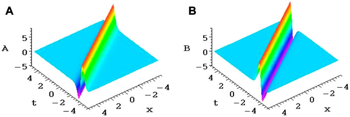
FIGURE 1. (A,B) are single soliton structures of Eqs 27, 28, respectively, when the parameters taken as Eq. 29.
When N = 2, Eq. 24 becomes as follows:
with
The corresponding two-soliton solution can be obtained by substituting Eq. 30 with Eqs 31, 32 into Eq. 19. From the perspective of algebra, it is natural to consider the simplification of the function of Eq. 30 by quantifying the double variables of the hyperbolic function into single variables, that is, k1 = ±k2, ω1 = ±ω2. These four cases may produce the corresponding soliton or breather solutions for the Alice–Bob system, respectively. Two typical cases are presented here for N = 2. Figure 2 presents this structure when the related parameters are taken through the real constants as follows:
Therefore,
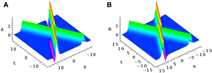
FIGURE 2. (A,B) are the two-soliton structures of the Alice-Bob systems (9) and (10), respectively through Eq. 19 after selecting the conditions are Eqs 33, 34.
It is not difficult to find that Eq. 34 is coupled by two hyperbolic functions similar to Eq. 26, and its image also shows this phenomenon.
On the other hand, by restricting the parameters k1, k2 to the assumed units on the two-soliton solution, the breather can be obtained. For example, by setting the following parameters
the following equation can be derived:
Here, the cosine part of Eq. 36 makes the Alice–Bob system periodic, and the corresponding breather structure is obtained, as shown in Figure 3.
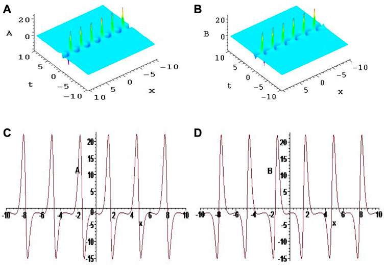
FIGURE 3. Breather structures of the Alice–Bob system (9) and (10) through Eq. 19 after selecting the conditions are Eqs 35, 36. (C,D) are the corresponding sectional plots of (A,B) at t =0, respectively.
When N = 3, Eq. 24 has the following more complicated situation:
with
and
Based on the selecting parameters b, c, k1, k2, δ1, and δ2 of Eqs 33, 35, two kinds of interactions for the solitons can be constructed by considering the following equation:
and
For this time, K{i}(i = 0, 1, 2, 3) are expressed as follows:
and
The corresponding functions of Eq. 37 are expressed as follows:
and
Figure 4 and Figure 5 show two interaction structures of the Alice–Bob systems (9) and (10) through Eqs 42, 43.
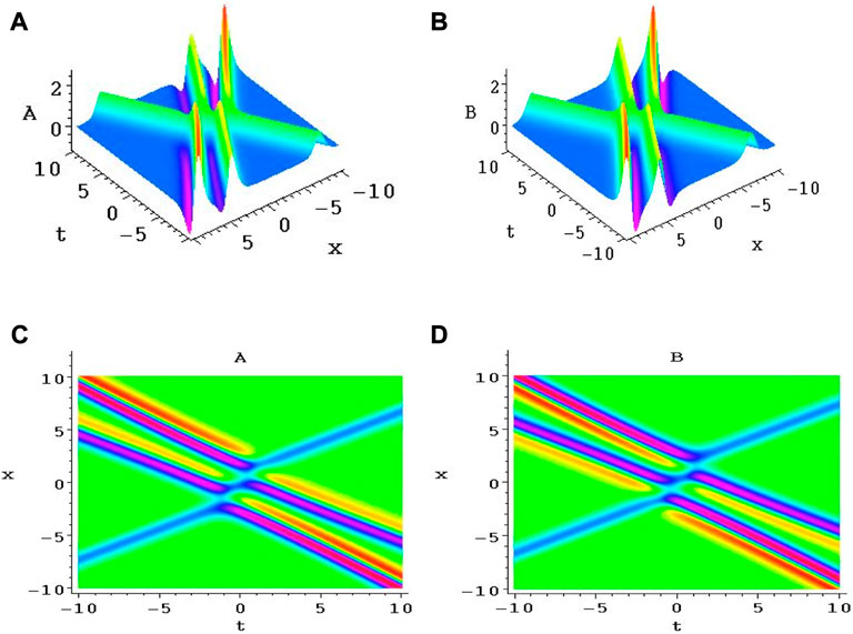
FIGURE 4. (A,B) are the interaction structures of three solitons for the Alice–Bob systems (9) and (10) through Eq. 42. (C,D) are the corresponding density plots of (A,B), respectively.
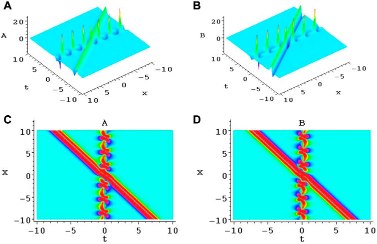
FIGURE 5. (A,B) are the interaction structures between the breather and one-soliton structures for the Alice–Bob systems (9) and (10) through Eq. 43. (C,D) are the corresponding density plots of (A,B), respectively.
The Alice–Bob systems (9) and (10) have a series of rational solutions and hence contain the corresponding lump structures. For this purpose, we introduce the following polynomial function:
where
When N = 1, Eq. 44 has the following simple form:
When
the lump solution of the Alice–Bob systems (9) and (10) has the following rational form:
which is obtained through the Bäcklund transformation (19) (Figure 6).
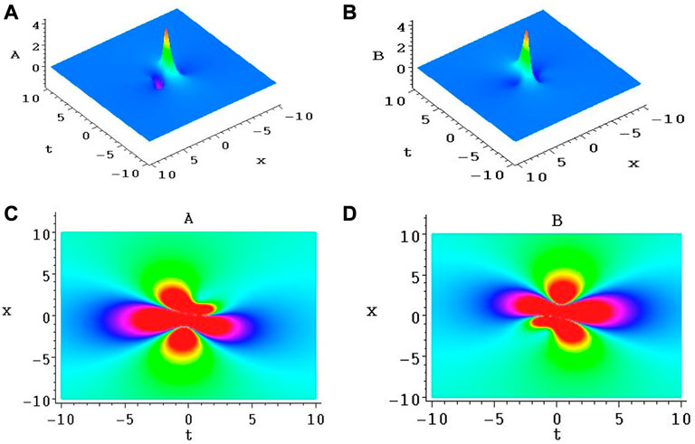
FIGURE 6. (A,B) are two lump structures of A and B from Eqs 47, 48. (C,D) are the corresponding density plots of (A,B), respectively.
When N = 2, Eq. 44 has the following function form:
A pair of lumps of A and B for the Alice–Bob systems (9) and (10) can be shown after the constants are taken as b = c = a0,0 = 1, just as Eq. 46, while
These two pairs of lumps for the Alice–Bob systems (9) and (10) through Eq. 19, Eq. 49, and Eq. 50 are shown in Figure 7.
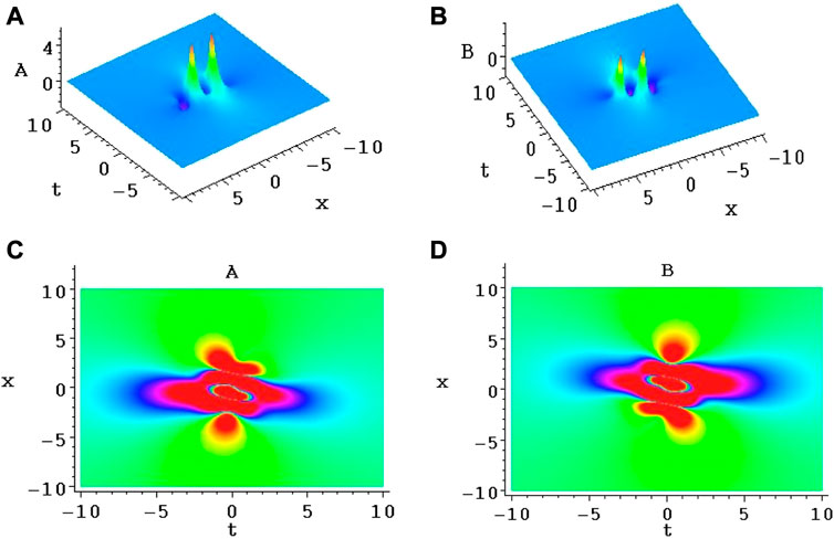
FIGURE 7. (A,B) are two pairs of lumps for the Alice–Bob systems (9) and (10) through Eqs 19, 49, 50. (C,D) are the corresponding density plots of (A,B), respectively.
When N = 3, Eq. 44 has the more complicated function form:
The lumps of A and B for the Alice–Bob systems (9) and (10) can also be constructed after the constants b = c = a0,0 = 1; therefore, the following equations are obtained:
These lump structures of the Alice–Bob systems (9) and (10) obtained through Eqs 19, 51, and 52 are shown in Figure 8.
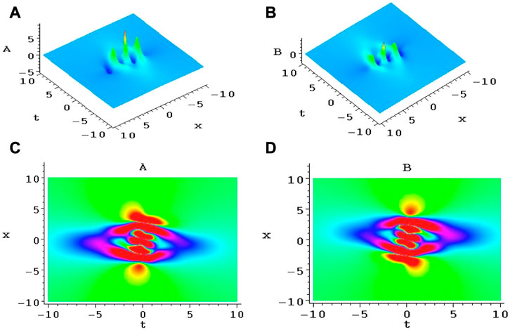
FIGURE 8. (A,B) are lump structures of A and B from Eqs 9, 10 through Eqs 19, 51, and 52. (C,D) are the corresponding density plots of (A,B), respectively.
In this paper, according to the (1 + 1)-dimensional Boussinesq Eq. 3, the Alice–Bob systems (9) and (10) for this equation are first derived through the Lax pair and the dark parameterization approach. This non-local system owns the bilinear form and may exist in the explicit solution. Therefore, the N-soliton solutions of the Alice–Bob systems (9) and (10) are presented with the aid of an undetermined function f after introducing an extended Bäcklund transformation. Typically, the auxiliary function can be taken as the hyperbolic function or rational function. These two kinds of functions induce the system having solutions that satisfy
The original contributions presented in the study are included in the article/Supplementary Material; further inquiries can be directed to the corresponding author.
PD: writing—original draft and software. Z-YM: supervision and funding acquisition. J-XF: conceptualization and software. W-PC: formal analysis and investigation.
This work was supported by the National Natural Science Foundation of China (11775104) and the Zhejiang Province Natural Science Foundation of China (2022SJGYZC01).
The authors declare that the research was conducted in the absence of any commercial or financial relationships that could be construed as a potential conflict of interest.
All claims expressed in this article are solely those of the authors and do not necessarily represent those of their affiliated organizations, or those of the publisher, the editors, and the reviewers. Any product that may be evaluated in this article, or claim that may be made by its manufacturer, is not guaranteed or endorsed by the publisher.
1. Bender CM, Boettcher S. Real spectra in non-hermitian Hamiltonians HavingPTSymmetry. Phys Rev Lett (1998) 80:5243–6. doi:10.1103/physrevlett.80.5243
2. Ablowitz MJ, Musslimani ZH. Integrable nonlocal nonlinear Schrödinger equation. Phys Rev Lett (2013) 110:064105–5. doi:10.1103/physrevlett.110.064105
3. Lou SY. Alice-Bob systems,
4. Lou SY. Prohibitions caused by nonlocality for nonlocal Boussinesq-KdV type systems. Stud Appl Math (2019) 142:1–16. doi:10.1111/sapm.12265
5. Li H, Lou SY. Multiple soliton solutions of Alice-Bob Boussinesq equations. Chin Phys Lett (2019) 36:050501–5. doi:10.1088/0256-307x/36/5/050501
6. Zhao QL, Lou SY, Jia M. Solitons and soliton molecules in two nonlocal Alice-Bob Sawada-Kotera systems. Commun Theor Phys (2020) 72:085005–7. doi:10.1088/1572-9494/ab8a0e
7. Jia M, Lou SY. Exact PsTd invariant and PsTd symmetric breaking solutions, symmetry reductions and Bäcklund transformations for an AB-KdV system. Phys Lett A (2018) 382:1157–66. doi:10.1016/j.physleta.2018.02.036
8. Wazwaz AM. Multiple soliton solutions and multiple complex soliton solutions for two distinct Boussinesq equations. Nonlinear Dyn (2016) 85:731–7. doi:10.1007/s11071-016-2718-0
9. Yang D, Lou SY, Yu WF. Interactions between solitons and cnoidal periodic waves of the Boussinesq equation. Commun Theor Phys (2013) 60:387–90. doi:10.1088/0253-6102/60/4/01
10. Adem AR, Yildirim Y, Yasar E. Soliton solutions to the non-local Boussinesq equation by multiple exp-function scheme and extended Kudryashov’s approach. Pramana-j Phys (2019) 92:24–11. doi:10.1007/s12043-018-1679-x
11. Fei JX, Ma ZY, Cao WP. Controllable symmetry breaking solutions for a nonlocal Boussinesq system. Sci Rep-uk (2019) 9:19667–14. doi:10.1038/s41598-019-56093-8
12. Cao WP, Fei JX, Li JY. Symmetry breaking solutions to nonlocal Alice-Bob Kadomtsev-Petviashivili system. Chaos Soliton Fract (2021) 144:110653–8. doi:10.1016/j.chaos.2021.110653
13. Wu WB, Lou SY. Exact solutions of an Alice-Bob KP equation. Commun Theor Phys (2019) 71:629–32. doi:10.1088/0253-6102/71/6/629
14. Lou SY. Dark parameterizations, equivalent partner fields and integrable systems. Commun Theor Phys (2011) 55:743–6. doi:10.1088/0253-6102/55/5/02
15. Peng L, Yang XD, Lou SY. Integrable KP coupling and its exact solution. Commun Theor Phys (2012) 58:1–4. doi:10.1088/0253-6102/58/1/01
16. Cao WP, Fei JX, Ma ZY, Liu Q. Bosonization and new interaction solutions for the coupled Korteweg-de Vries system. Wave Random Complex (2020) 30:130–41. doi:10.1080/17455030.2018.1489565
17. Fei JX, Cao WP, Ma ZY. Dark parameterization approach to the Benjamin Ono equation. Int J Mod Phys B (2020) 34:2050247–8. doi:10.1142/s0217979220502471
18. Hirota R. Exact solution of the Korteweg-de Vries equation for multiple collisions of solitons. Phys Rev Lett (1971) 27:1192–4. doi:10.1103/physrevlett.27.1192
20. Clarkson PA, Dowie E. Rational solutions of the Boussinesq equation and applications to rogue waves. Trans Math Appl (2017) 1:1–26. doi:10.1093/imatrm/tnx003
Keywords: (1+1)-dimensional Alice–Bob Boussinesq equation, Lax pair, Bäcklund transformation, PsTd symmetry-breaking solution, hybrid structure
Citation: Dong P, Ma Z-Y, Fei J-X and Cao W-P (2023) The shifted parity and delayed time-reversal symmetry-breaking solutions for the (1+1)-dimensional Alice–Bob Boussinesq equation. Front. Phys. 11:1137999. doi: 10.3389/fphy.2023.1137999
Received: 05 January 2023; Accepted: 16 February 2023;
Published: 09 March 2023.
Edited by:
Yunqing Yang, Zhejiang Ocean University, ChinaReviewed by:
Sakkaravarthi Karuppaiya, Asia Pacific Center for Theoretical Physics (APCTP), Republic of KoreaCopyright © 2023 Dong, Ma, Fei and Cao. This is an open-access article distributed under the terms of the Creative Commons Attribution License (CC BY). The use, distribution or reproduction in other forums is permitted, provided the original author(s) and the copyright owner(s) are credited and that the original publication in this journal is cited, in accordance with accepted academic practice. No use, distribution or reproduction is permitted which does not comply with these terms.
*Correspondence: Zheng-Yi Ma, bWEtemhlbmd5aUAxNjMuY29t
Disclaimer: All claims expressed in this article are solely those of the authors and do not necessarily represent those of their affiliated organizations, or those of the publisher, the editors and the reviewers. Any product that may be evaluated in this article or claim that may be made by its manufacturer is not guaranteed or endorsed by the publisher.
Research integrity at Frontiers
Learn more about the work of our research integrity team to safeguard the quality of each article we publish.