A novel zeroing neural network for dynamic sylvester equation solving and robot trajectory tracking

To solve the theoretical solution of dynamic Sylvester equation (DSE), we use a fast convergence zeroing neural network (ZNN) system to solve the time-varying problem. In this paper, a new activation function (AF) is proposed to ensure fast convergence in predefined times, as well as its robustness in the presence of external noise perturbations. The effectiveness and robustness of this zeroing neural network system is analyzed theoretically and verified by simulation results. It was further verified by the application of robotic trajectory tracking.

1 Introduction

Recurrent neural networks (RNN) have been extensively studied and applied in many scientific and engineering fields in the past two decades, such as automatic control theory [1], image processing [2, 3], data processing [4], and matrix equations solving [5–7]. The Sylvester equation plays a very important role in mathematics and control fields, and it will be involved in many practical applications [8–12].

The theoretical solution of the general Sylvester equation can be obtained through the conventional gradient descent method [13]. Using the norm of the error matrix as a performance indicator, a neural network is evolved along the gradient descent direction so that the error norm in the fixed-constant case vanishes to zero over time [14]. However, in the time-varying case, due to the lack of velocity compensation for the time-varying parameters, the error norm may not converge to zero, even after an infinitely long time. To solve the problem of solving the dynamic Sylvester equations, a design method based on zeroing neural network system is adopted. Zeroing neural network is a special recurrent neural network proposed by Zhang et al. [6, 15], and plays a crucial role in solving various dynamic problem fields. Generally speaking, zeroing neural networks have better accuracy and higher efficiency than recurrent neural networks based on gradient descent in solving time-varying problems [16, 17]. In recent years, ZNN has been studied more and more, and many new models have been developed. For example, the VP-CZNN in Ref. [5] and the FT-VP-CZNN in Ref. [18] realize super exponential convergence, and the ZNN model activated by SBPAF in Ref. [19] realizes finite-time convergence.

There are often many kinds of external noise interference in real life, and most neural network systems do not consider the tolerance problem of noise, which reduces the effect of dynamic systems. Through the above discussion analysis, a new activation function can be introduced to improve the performance of the whole system. At the same time, it can also ensure the predefined time convergence and noise resistance.

The rest of this paper is organized as follows. In Section 2, we introduce zeroing neural network model and dynamic Sylvester equation. In Section 3, we review some activation functions and propose a new activation function with predefined time convergence under noise interference. In Section 4, we focus on the predefined-time convergence and anti-noise capability of the model that we established. In Section 5, we verify the theory through simulation experiments of solving the dynamic Sylvester equations and the trajectory tracking problem of the robotic arm. Finally, we give a brief conclusion to the paper in Section 6. In addition, all the abbreviations used in this work are listed in the following Table 1.

TABLE 1

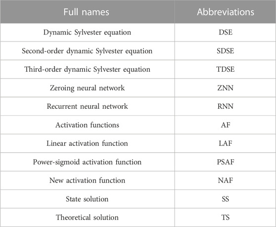
TABLE 1. All the abbreviations used in this work.

2 ZNN model and dynamic sylvester equation

In this work, we are concerned with the Sylvester equation, and its general expression is directly given as:

$A\left(t\right)X\left(t\right)-X\left(t\right)B\left(t\right)=-C\left(t\right)\in R^{n\times n}(1)$

where $A\left(t\right)\in R^{n\times n},B\left(t\right)\in R^{n\times n},C\left(t\right)\in R^{n\times n}$ stand for known coefficient matrices, and $X\left(t\right)\in R^{n\times n}$ stands for an unknown matrix we need to solve.

To solve the Sylvester equation, we define an error function:

$E\left(t\right)=A\left(t\right)X\left(t\right)-X\left(t\right)B\left(t\right)+C\left(t\right)\in R^{n\times n}(2)$

If each elements of the error function E(t) converges to 0, we can obtain the theoretical solution X(t). To make the error function converge to 0, the ZNN design formula is designed by the following derivative equation:

$\frac{d\left(E\left(t\right)\right)}{d\left(t\right)}=-\gamma \phi \left(E\left(t\right)\right)(3)$

where $\phi \left(\cdot \right)\in R^{n\times n}$ stands for an array of the activation function, and $\gamma >0$ are a known adjustable parameter which adjust the convergence rate.

The time derivative of the error function is defined as:

$\stackrel{•}{E}\left(t\right)=A\left(t\right)\stackrel{•}{X}\left(t\right)+\stackrel{•}{A}\left(t\right)X\left(t\right)-\stackrel{•}{X}\left(t\right)B\left(t\right)-X\left(t\right)\stackrel{•}{B}\left(t\right)+\stackrel{•}{C}\left(t\right)(4)$

Then, by substituting error function into the ZNN design formula and considering that the time derivative of the error function, the following ZNN model for Sylvester equation is derived:

$A\left(t\right)\stackrel{•}{X}\left(t\right)-\stackrel{•}{X}\left(t\right)B\left(t\right)=-\stackrel{•}{A}\left(t\right)X\left(t\right)+X\left(t\right)\stackrel{•}{B}\left(t\right)-\stackrel{•}{C}\left(t\right)-\gamma \phi \left(A\left(t\right)X\left(t\right)-X\left(t\right)B\left(t\right)+C\left(t\right)\right)(5)$

3 Activation function

The activation function is a monotonically increasing odd function and is a key component of the ZNN model. It has important implications for the convergence and robustness of the ZNN models. Especially in the presence of noise interference, the selection of an appropriate activation function can play a great positive role in the ZNN model. In the past decade, many activation functions have been proposed to improve the performance of neural networks, and different activation functions can be found to have different performance through comparison [20–22].

Several common activation functions.

1) Linear activation function (LAF)

$\varphi \left(x\right)=x(6)$

2) Power activation function

$\varphi \left(x\right)=x^p(7)$

with $p\ge 3$ indicating an odd integer.

3) Power-sigmoid activation function (PSAF)

$\varphi \left(x\right)=\left\{\begin{array}{cc}{x}^p& ,\left|x\right|\ge 1\\ \frac{1+\exp \left(-\xi \right)}{1-\exp \left(-\xi \right)}\frac{1-\exp \left(-\xi x\right)}{1+\exp \left(-\xi x\right)}& ,\left|x\right|<1\end{array}\right.(8)$

4) Sign-bi-power activation function

$\varphi \left(x\right)=\frac{1}{2}{\mathrm{s}\mathrm{g}\mathrm{n}}^{{\xi }_1}\left(x\right)+\frac{1}{2}{\mathrm{s}\mathrm{g}\mathrm{n}}^{{\xi }_2}\left(x\right)(9)$

where ${\xi }_1\in \left(\mathrm{0,1}\right)$ and ${\xi }_2>1$, $\mathrm{s}\mathrm{g}\mathrm{n}\left(\cdot \right)$ is defined as:

${\mathrm{s}\mathrm{g}\mathrm{n}}^n\left(x\right)=\left\{\begin{array}{c}{\left|x\right|}^n,x>0\\ 0,x=0\\ -{\left|x\right|}^n,x<0\end{array}\right.(10)$

Different activation functions have different convergence performance, and non-linear activation function generally possesses better performance than the linear activation function in the rate of the accelerated ZNN model convergence. All of the above activation functions can effectively improve the convergence rate, but they do not consider the noise factor. The convergence performance is greatly reduced in the presence of noise interference. Considering this factor, we propose a new activation function (NAF) with predefined time convergence under noise interference:

$\varphi \left(x\right)=\left(k_1{\left|x\right|}^p+k_2{\left|x\right|}^{\raisebox{1ex}{$1$}\!\left/ \!\raisebox{-1ex}{$p$}\right.}+k_3\right)\mathrm{s}\mathrm{g}\mathrm{n}\left(x\right)+k_4{x}^{2\lambda -1}(11)$

where $0<p<1,k_1>0,k_2>0,k_3>0,k_4>0,\lambda \in N+$, and $\mathrm{s}\mathrm{g}\mathrm{n}\left(\cdot \right)$ is defined as described above.

4 Network model and theoretical analysis

Before the main theoretical results of the ZNN are given, the following lemma is first presented as a basis for further discussion [5].

Lemma. There is a non-linear dynamical system such as $\stackrel{•}{X}\left(t\right)=g\left(x\left(t\right),t\right)$, $t\in \left[0,+\infty \right.)$, where g(t) is a non-linear function. If a continuous radial unbounded function $V:R^n\to R_{+}\cup \left\{0\right\}$ exists, making $U\left(\zeta \right)=0$ and any solution satisfied:

$\stackrel{•}{U}\left(t\right)\le -\tau U^{\varsigma }\left(\zeta \left(t\right)\right)-\rho U^{\mu }\left(\zeta \left(t\right)\right)(12)$

where $\tau >0,\rho >\mathrm{0,0}<\varsigma <1,\mu >0$ all are constants.

The predefined convergence time is:

$T_{\max }=\frac{1}{\tau \left(1-\varsigma \right)}+\frac{1}{\rho \left(\mu -1\right)}(13)$

Theorem 1. Starting with the random initial matrix, the exact solution of the ZNN model predefined convergence is as:

$t_c\le \frac{1}{\gamma k_1\left(1-p\right)}+\frac{1}{\gamma k_2\left(\raisebox{1ex}{$1$}\!\left/ \!\raisebox{-1ex}{$p$}\right.-1\right)}(14)$

where $\gamma ,k_1,k_2,p$ stand for the preset parameters.

Proof of Theorem 1. The ZNN model can be represented as $\stackrel{•}{E}\left(t\right)=-\gamma \varphi \left(E\left(t\right)\right)$, where $E\left(t\right)$ represents error function, and subsystem (i, j) can be expressed as:

$\stackrel{•}{e_{i,j}}\left(t\right)=-\gamma \varphi \left(e_{i,j}\left(t\right)\right)(15)$

with $i,j\in \left\{\mathrm{1,2},...,n\right\}$. If the subsystem possesses predefined time stability, the ZNN model also possesses it. To prove the stability of the predefined time, we define a Lyapunov function as:

$u\left(t\right)=\left|e_{i,j}\left(t\right)\right|(16)$

The time derivative is:

$\begin{array}{l}\stackrel{•}{u}\left(t\right)=-\stackrel{•}{e_{i,j}}\left(t\right)\mathrm{s}\mathrm{g}\mathrm{n}\left(e_{i,j}\left(t\right)\right)=-\gamma \varphi \left(e_{i,j}\left(t\right)\right)\mathrm{s}\mathrm{g}\mathrm{n}\left(e_{i,j}\left(t\right)\right)\\ =-\gamma \left(k_1{\left|e_{i,j}\left(t\right)\right|}^p+k_2{\left|e_{i,j}\left(t\right)\right|}^{\raisebox{1ex}{$1$}\!\left/ \!\raisebox{-1ex}{$p$}\right.}+k_4{\left|e_{i,j}\left(t\right)\right|}^{2\lambda -1}+k_3\right)\\ \le -\gamma \left(k_1{\left|e_{i,j}\left(t\right)\right|}^p+k_2{\left|e_{i,j}\left(t\right)\right|}^{\raisebox{1ex}{$1$}\!\left/ \!\raisebox{-1ex}{$p$}\right.}\right)\\ =-\gamma \left(k_1{u}^p\left(t\right)+k_2{u}^{\raisebox{1ex}{$1$}\!\left/ \!\raisebox{-1ex}{$p$}\right.}\left(t\right)\right)\end{array}(17)$

Comparing with the lemma, predefined convergence time is available:

$t_c\le \frac{1}{\gamma k_1\left(1-p\right)}+\frac{1}{\gamma k_2\left(\raisebox{1ex}{$1$}\!\left/ \!\raisebox{-1ex}{$p$}\right.-1\right)}(18)$

Because there may be various disturbances in reality, the following ZNN model perturbed by noise is studied:

$A\left(t\right)\stackrel{•}{X}\left(t\right)-\stackrel{•}{X}\left(t\right)B\left(t\right)=-\stackrel{•}{A}\left(t\right)X\left(t\right)+X\left(t\right)\stackrel{•}{B}\left(t\right)-\stackrel{•}{C}\left(t\right)-\gamma \phi \left(A\left(t\right)X\left(t\right)-X\left(t\right)B\left(t\right)+C\left(t\right)\right)+Y\left(t\right)(19)$

where Y(t) represents an additional noise.

Case 1. Dynamic bounded vanishing noise.

Theorem 2. There is a dynamically bounded vanishing noise, where its elements (i, j) satisfy $\left|y_{i,j}\left(t\right)\right|\le \delta \left|e_{i,j}\left(t\right)\right|$ and $\delta \in \left(0,+\infty \right),\left|e_{i,j}\left(t\right)\right|$ is the absolute value of the element (i, j) in the error function E (t). Starting with a random initial matrix $X\left(0\right)\in R^{n\times n}$, If it satisfy $\gamma k_4\ge \delta$, it will output exact solutions of the time-varying Sylvester equation at the predefined time $t_c$.

$t_c\le \frac{1}{\gamma k_1\left(1-p\right)}+\frac{1}{\gamma k_2\left(\raisebox{1ex}{$1$}\!\left/ \!\raisebox{-1ex}{$p$}\right.-1\right)}(20)$

Proof of Theoreim 2. The ZNN model which is perturbed by noise can be reduced to $\stackrel{•}{E}\left(t\right)=-\gamma \varphi \left(E\left(t\right)\right)+Y\left(t\right)$, The subsystem (i, j) is expressed as:

${\stackrel{•}{e}}_{i,j}\left(t\right)=-\gamma \varphi \left(e_{i,j}\left(t\right)\right)+y_{i,j}\left(t\right)(21)$

where $y_{i,j}\left(t\right)$ stands for the element (i, j) of matrix Y(t).

To prove the predefined time stability of the subsystem subject to noise perturbation, we define a Lyapunov function as:

$u\left(t\right)={\left[e_{i,j}\left(t\right)\right]}^2(22)$

The time derivative is:

$\begin{array}{l}\stackrel{•}{u}\left(t\right)=2e_{i,j}\left(t\right){\stackrel{•}{e}}_{i,j}\left(t\right)=2e_{i,j}\left(t\right)(-\gamma \varphi (e_{i,j}\left(t\right))+y_{i,j}\left(t\right))\\ =-2\gamma \left(k_1{\left|e_{i,j}\left(t\right)\right|}^{p+1}+k_2{\left|e_{i,j}\left(t\right)\right|}^{\raisebox{1ex}{$1$}\!\left/ \!\raisebox{-1ex}{$p$}\right.+1}\right)-2\gamma k_3\left|e_{i,j}\left(t\right)\right|+2\left(e_{i,j}\left(t\right)y_{i,j}\left(t\right)-\gamma k_4{\left|e_{i,j}\left(t\right)\right|}^{2\left(2\lambda -1\right)}\right)\\ \le -2\gamma \left(k_1{\left|e_{i,j}\left(t\right)\right|}^{p+1}+k_2{\left|e_{i,j}\left(t\right)\right|}^{\raisebox{1ex}{$1$}\!\left/ \!\raisebox{-1ex}{$p$}\right.+1}\right)+2\left(\delta {\left|e_{i,j}\left(t\right)\right|}^2-\gamma k_4{\left|e_{i,j}\left(t\right)\right|}^{2\left(2\lambda -1\right)}\right)\\ \le -2\gamma \left(k_1{\left|e_{i,j}\left(t\right)\right|}^{p+1}+k_2{\left|e_{i,j}\left(t\right)\right|}^{\raisebox{1ex}{$1$}\!\left/ \!\raisebox{-1ex}{$p$}\right.+1}\right)\\ =-2\gamma \left(k_1{u}^{\left(p+1\right)/2}\left(t\right)+k_2{u}^{\left(\raisebox{1ex}{$1$}\!\left/ \!\raisebox{-1ex}{$p$}\right.+1\right)/2}\left(t\right)\right)\end{array}(23)$

with $\lambda$ is positive integer. Therefore, $2\left(2\lambda -1\right)$ is certainly greater than or equal to 2. If it satisfy $\gamma k_4\ge \delta$, the upper formula must hold.

Comparing with the lemma, predefined convergence time is available:

$t_c\le \frac{1}{\gamma k_1\left(1-p\right)}+\frac{1}{\gamma k_2\left(\raisebox{1ex}{$1$}\!\left/ \!\raisebox{-1ex}{$p$}\right.-1\right)}(24)$

Case 2. Dynamic bounded non-vanishing noise.

Theorem 3. There exists a dynamically bounded non-vanishing noise, where its elements (i, j) satisfy $\left|y_{i,j}\left(t\right)\right|\le \delta$, and $\delta \in \left(0,+\infty \right)$. Starting with a random initial matrix, if it satisfy $\gamma k_3\ge \delta$, it will output exact solutions of the time-varying Sylvester equation at the predefined time $t_c$.

$t_c\le \frac{1}{\gamma k_1\left(1-p\right)}+\frac{1}{\gamma k_2\left(\raisebox{1ex}{$1$}\!\left/ \!\raisebox{-1ex}{$p$}\right.-1\right)}(25)$

Proof of Theorem 3. The additive noise is just different, comparing with Theorem 2. Therefore, we still choose the following Lyapunov function:

$u\left(t\right)={\left[e_{i,j}\left(t\right)\right]}^2(26)$

The time derivative is:

$\begin{array}{l}\stackrel{•}{u}\left(t\right)=2e_{i,j}\left(t\right){\stackrel{•}{e}}_{i,j}\left(t\right)=2e_{i,j}\left(t\right)\left(-\gamma \varphi \left(e_{i,j}\left(t\right)\right)+y_{i,j}\left(t\right)\right)\\ =-2\gamma \left(k_1{\left|e_{i,j}\left(t\right)\right|}^{p+1}+k_2{\left|e_{i,j}\left(t\right)\right|}^{\raisebox{1ex}{$1$}\!\left/ \!\raisebox{-1ex}{$p$}\right.+1}\right)-2\gamma k_4{\left|e_{i,j}\left(t\right)\right|}^{2\left(2\lambda -1\right)}+2\left(e_{i,j}\left(t\right)y_{i,j}\left(t\right)-\gamma k_3\left|e_{i,j}\left(t\right)\right|\right)\\ \le -2\gamma \left(k_1{\left|e_{i,j}\left(t\right)\right|}^{p+1}+k_2{\left|e_{i,j}\left(t\right)\right|}^{\raisebox{1ex}{$1$}\!\left/ \!\raisebox{-1ex}{$p$}\right.+1}\right)+2\left(\delta \left|e_{i,j}\left(t\right)\right|-\gamma k_3\left|e_{i,j}\left(t\right)\right|\right)\\ \le -2\gamma \left(k_1{\left|e_{i,j}\left(t\right)\right|}^{p+1}+k_2{\left|e_{i,j}\left(t\right)\right|}^{\raisebox{1ex}{$1$}\!\left/ \!\raisebox{-1ex}{$p$}\right.+1}\right)\\ =-2\gamma \left(k_1{u}^{\left(p+1\right)/2}\left(t\right)+k_2{u}^{\left(\raisebox{1ex}{$1$}\!\left/ \!\raisebox{-1ex}{$p$}\right.+1\right)/2}\left(t\right)\right)\end{array}(27)$

If it satisfy $\gamma k_3\ge \delta$, the above formula is established.

Comparing with the lemma, predefined convergence time is available:

$t_c\le \frac{1}{\gamma k_1\left(1-p\right)}+\frac{1}{\gamma k_2\left(\raisebox{1ex}{$1$}\!\left/ \!\raisebox{-1ex}{$p$}\right.-1\right)}(28)$

According to the above discussion and analysis, it can be concluded that the proposed network model can effectively achieve the predefined time convergence, and can attain better performance in environments where noise disturbance exists.

5 Simulation effect verification

A network model based on a novel activation function is proposed above. Unlike the common activation function, this activation function can achieve predefined time convergence in a noisy environment. And we perform a convergence analysis for different types of noise. Then we will verify the convergence effect and compare it with the simulation effect of other common activation functions. Firstly, we apply the contrast by simulations of time-varying Sylvester equations.

5.1 Simulation 1: second order coefficient matrix

Generally, coefficient matrix A(t), B(t) and C(t) can be chosen randomly, as long as A(t) and B(t) are both invertible matrix. For no loss of generality, the following second-order matrices are selected:

$A\left(t\right)=\left(\begin{array}{l}\sin \left(2t\right)\cos \left(4t\right)\\ -\cos \left(4t\right)\sin \left(3t\right)\end{array}\right),B\left(t\right)=\left(\begin{array}{l}30\\ 12\end{array}\right),C\left(t\right)=\left(\begin{array}{l}\sin \left(4t\right)\cos \left(4t\right)\\ -\cos \left(4t\right)\sin \left(4t\right)\end{array}\right)$

For random initial state $X\left(0\right)\in {\left[\mathrm{2,2}\right]}^{2\times 2}$, the network model with the classical linear activation function, the power-sigmoid activation function, and the proposed activation function is simulated in a noise-free environment.

The results are presented in Figure 1. The following figures are the comparison of the state solution (SS) and the theoretical solution (TS) of the three activation functions in a noiseless environment, where the red dashed line represents the theoretical solution, and the blue solid line indicates the state solution. Each group of status figure is composed of four components, representing the four elements $\left(x_{11}{x}_{12};x_{21}{x}_{22}\right)$ in the matrix in turn.

FIGURE 1

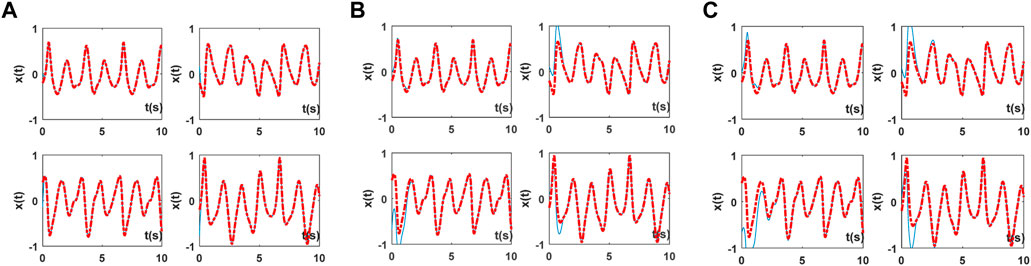
FIGURE 1. The comparison of the state solution and the theoretical solution: (A) SS of NAF for solving SDSE; (B) SS of PSAF for solving SDSE; (C) SS of LAF for solving SDSE.

The first set of graphs shows a comparison of the state solution produced by the newly proposed activation function with the theoretical solution. And the second and third sets of graphs represent the state contrast figures which are produced by the power-sigmoid activation function and linear activation function. It is obvious from the three groups that the state solutions produced by the newly proposed activation function are closer to the theoretical values.

The following sets of graphs in Figure 2 show the residual graphs generated by the three activation functions in different noise environments, where the blue line represents the newly proposed activation function, the red line represents the power-sigmoid activation function, and the yellow line represents the linear activation function. The first figure shows the residual figure in a noiseless environment; the remaining two figures are the residual figures in the presence of an external noise of y(t) = 0.3t and y (t) = cos (t). Obviously, the newly proposed activation function can achieve faster convergence and possesses a better anti-noise interference ability.

FIGURE 2

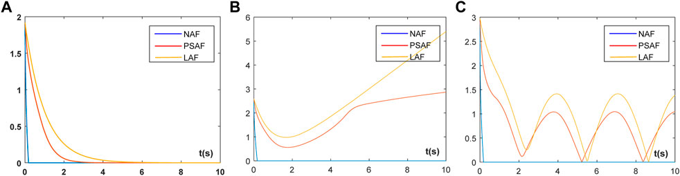
FIGURE 2. Residual graphs generated by the three activation function: (A) Simulated residual errors of ZNN for solving SDSE without noise; (B) Simulated residual errors of ZNN for solving SDSE with y(t) = 0.3t; (C) Simulated residual errors of ZNN for solving SDSE with y(t) = cos(t).

5.2 Simulation 2: Third order coefficient matrix

The principle as above, coefficient matrix A(t), B(t) and C(t) are chosen randomly, as long as A(t) and B(t) are both invertible matrix. For no loss of generality, select following random third-order matrices:

$A\left(t\right)=\left(\begin{array}{l}\sin \left(2t\right)\sin \left(2t\right)\cos \left(t\right)\\ \cos \left(3t\right)\sin \left(2t\right)-\sin \left(2t\right)\\ \sin \left(t\right)\cos \left(2t\right)\sin \left(2t\right)\end{array}\right),B\left(t\right)=\left(\begin{array}{lll}10& 0& 5\\ 0& 20& 10\\ 0& 15& 20\end{array}\right)C\left(t\right)=\left(\begin{array}{l}\sin \left(2t\right)\sin \left(2t\right)\cos \left(3t\right)\\ \cos \left(3t\right)\sin \left(2t\right)-\sin \left(3t\right)\\ -\sin \left(t\right)\cos \left(3t\right)\sin \left(2t\right)\end{array}\right)$

For random initial state $X\left(0\right)\in {\left[\mathrm{1,1}\right]}^{3\times 3}$, the network model with the classical linear activation function, the power-sigmoid activation function, and the proposed activation function is simulated in the presence of noise (Y(t) = 0.5t) environment.

The results are presented in Figure 3. The figure shows the comparison of the state solutions and the theoretical solutions of the three activation functions in this environment, where the red dashed line represents the theoretical solution, and the blue solid line indicates the state solution. Each group of status figure is composed of nine components, representing the nine elements $\left(x_{11}{x}_{12}{x}_{13};x_{21}{x}_{22}{x}_{23};x_{31}{x}_{32}{x}_{33}\right)$ in the matrix in turn.

FIGURE 3

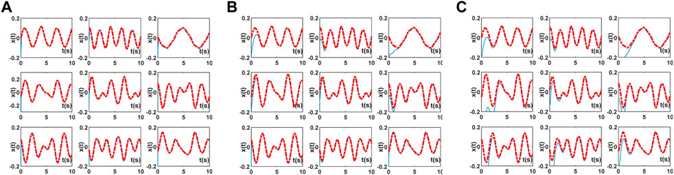
FIGURE 3. The comparison of the state solution and the theoretical solution: (A) SS of NAF for solving TDSE; (B) SS of PSAF for solving TDSE; (C) SS of LAF for solving TDSE.

The first set of graphs shows a comparison of the state solution produced by the newly proposed activation function with the theoretical solution. The second and third sets of graphs represent the state contrast figures which are produced by the power-sigmoid activation function and linear activation function. It is obvious from the three groups that the state solutions produced by the newly proposed activation function are closer to the theoretical values.

The supra sets of graphs in Figure 4 show the residual graphs generated by the three activation functions in different noise environments, where the blue line represents the newly proposed activation function, the red line represents the power-sigmoid activation function, and the yellow line represents the linear activation function. The first figure shows the residual figure in a noiseless environment; the remaining two figures are the residual figures in the presence of an external noise of y(t) = 0.3t and y (t) = cos(t). Obviously, the newly proposed activation function can achieve faster convergence and possesses better anti-noise interference ability.

FIGURE 4

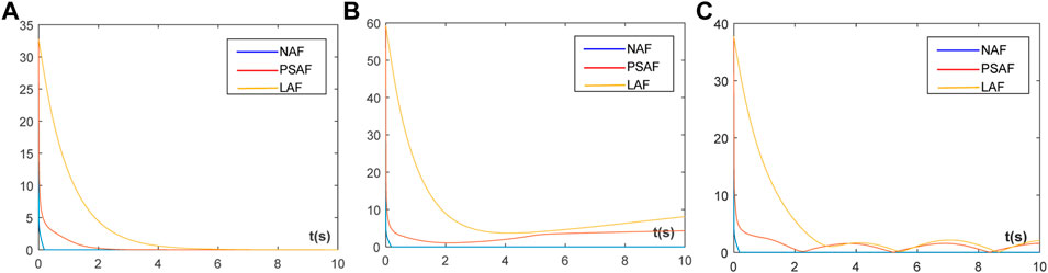
FIGURE 4. Residual graphs generated by the three activation function: (A) Simulated residual errors of ZNN for solving TDSE without noise; (B) Simulated residual errors of ZNN for solving TDSE with y(t) = 0.3t; (C) Simulated residual errors of ZNN for solving TDSE with y(t) = cos(t).

5.3 Simulation 3: Mechanical arm trajectory tracking

The joint angle vector θ of the robotic arm and the actual trajectory L of the end actuator are related to:

$L=f\left(\theta \right)(29)$

where $f\left(\cdot \right)$ is a known non-linear one-to-many function between the joint angle and the actual trajectory of end-effector. Given the movement path L of the end-effector, the motion change of the corresponding joint angle vector θ can be determined.

From the time-varying view, the equations of motion of the robotic arm can be expressed as:

$L\left(t\right)=f\left(\theta \left(t\right)\right)(30)$

The track-tracking problem eventually turns into a speed problem. Therefore, the two sides of the above equation are guided to obtain the motion equation of the mechanical arm at the velocity level:

$\stackrel{•}{L}\left(t\right)=J\left(\theta \right)\stackrel{•}{\theta }\left(t\right)(31)$

where $J\left(\theta \right)$ represents a Jacobian matrix $J\left(\theta \right)=\partial f\left(\theta \right)/\partial \theta$. After introducing the Jacobian matrix, the time-varying joint angular velocity $\stackrel{•}{\theta }\left(t\right)$ and the mechanical arm end time-varying velocity $\stackrel{•}{L}\left(t\right)$ can be regarded as a linear relationship. Generally, $\stackrel{•}{L}\left(t\right)$ is known quantity and $\stackrel{•}{\theta }\left(t\right)$ is unknown quantity. Thus, the upper equation belongs to an inversion equation of motion and we can consider the trajectory tracking problem as a problem of solving a time-varying linear matrix equation.

The proposed network model is used to solve the time-varying problem and to construct the corresponding model:

$J\left(\theta \right)\stackrel{•}{\theta }\left(t\right)=\stackrel{•}{L}\left(t\right)-\gamma \varphi \left(L\left(t\right)-J\left(\theta \right)\theta \left(t\right)\right)+y\left(t\right)(32)$

where y(t) is additive noise and set to y(t) = 0.1t.

The expected tracking trajectory of the mechanical arm is a four-pointed star type, and the simulations in noisy environments are shown in Figure 5. The first graph in Figure 5 depicts the whole track schematic of the mechanical arm, and the second figure illustrates traced trajectory of it from the top perspective. The movement trajectory of the mobile platform is described in (c). Furthermore, a contrast drawing between expected path and actual trajectory is exhibited subsequently. Finally, the tracking error of this test in three dimensions is captured in (e). Therefore, the novel neural network model can accurately complete the trajectory tracking with small error under the noise polluted environment.

FIGURE 5

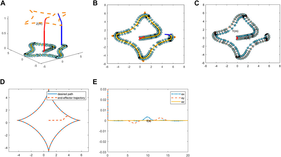
FIGURE 5. Simulations of mechanical arm tracking trajectory: (A) The whole track schematic; (B) Top plot of the traced trajectory; (C) Movement trajectory of the mobile platform; (D) Expected path and actual trajectory contrast; (E) Tracking error.

6 Conclusion

In this paper, we propose a zeroing neural network model by introducing a novel activation function. Through the theoretical analysis and simulation verification, the network model possesses the characteristics of predefined time convergence and strong noise resistance. In dealing with the problem of solving the dynamical Sylvester equations, it has faster convergence rate, higher accuracy and better robustness, comparing with several classical network models constructed with the activation functions. Moreover, the effectiveness and reliability of the network model have been validated by theoretical analysis and simulation in the robotic arm trajectory tracking problem.

In addition, there are some difficulties in future research. On the one hand, in the interest of improving the effectiveness of ZNN model, the structure require further optimized, such as designing other new outstanding activation functions and convergence factor. On the other hand, for the sake of improving the practicality of the ZNN model, it is necessary to expand the practical application scope of the model to other scientific and engineering fields, such as applying it to time-varying electronic circuits, chaotic systems, multi-agent research, chaotic systems.

Data availability statement

The original contributions presented in the study are included in the article/Supplementary Material, further inquiries can be directed to the corresponding authors.

Author contributions

Conceptualization, LZ and HS; methodology, HS; validation, LZ, XL, and XY; formal analysis, LZ; writing—original draft preparation, HS; writing—review and editing, LZ and XL; visualization, XY; supervision, ZT and HL. All authors have read and agreed to the published version of the manuscript.

Funding

This research was funded by National Natural Science Foundation of China, grant number 61875054; Natural Science Foundation of Hunan Province, grant number 2020JJ4315 and 2020JJ5199; Scientific Research Fund of Hunan Provincial Education Department, grant number 20B216 and 20C0786.

Conflict of interest

The authors declare that the research was conducted in the absence of any commercial or financial relationships that could be construed as a potential conflict of interest.

Publisher’s note

All claims expressed in this article are solely those of the authors and do not necessarily represent those of their affiliated organizations, or those of the publisher, the editors and the reviewers. Any product that may be evaluated in this article, or claim that may be made by its manufacturer, is not guaranteed or endorsed by the publisher.

References

1. Li S, Zhang Y, Jin L. Kinematic control of redundant manipulators using neural networks. IEEE Trans Neural Netw Learn Syst (2017) 28:2243–54. doi:10.1109/tnnls.2016.2574363

PubMed Abstract | CrossRef Full Text | Google Scholar

2. Nazemi A. A capable neural network framework for solving degenerate quadratic optimization problems with an application in image fusion. Neural Process Lett (2017) 47:167–92. doi:10.1007/s11063-017-9640-4

CrossRef Full Text | Google Scholar

3. Yu. F, Kong X, Mokbel AAM, Yao. W, Cai S. Complex dynamics, hardware implementation and image encryption application of multiscroll memeristive Hopfield neural network with a novel local active memeristor. IEEE Trans Circuits Systems--II: Express Briefs. (2023) 70:326–30. doi:10.1109/tcsii.2022.3218468

CrossRef Full Text | Google Scholar

4. Yu. F, She H, Yu. Q, Kong X, Sharma PK, Cai S. Privacy protection of medical data based on multi-scroll memristive Hopfield neural network. In: IEEE Transactions on Network Science and Engineering; 23 November 2022 (2022). doi:10.1109/TNSE.2022.3223930

CrossRef Full Text | Google Scholar

5. Li W, Liao B, Xiao L, A recurrent neural network with predefined-time convergence and improved noise tolerance for dynamic matrix square root finding. Neurocomputing (2019) 337:262–73. doi:10.1016/j.neucom.2019.01.072

CrossRef Full Text | Google Scholar

6. Zhao L, Jin J, Gong J. Robust zeroing neural network for fixed-time kinematic control of wheeled mobile robot in noise-polluted environment. Math Comput Simul (2021) 185:289–307. doi:10.1016/j.matcom.2020.12.030

CrossRef Full Text | Google Scholar

7. Jin J, Chen W, Chen C, Chen Z, Tang L, Chen L, et al. A predefined fixed-time convergence ZNN and its applications to time-varying quadratic programming solving and dual-arm manipulator cooperative trajectory tracking. IEEE Trans. Ind. Inform. (2022). doi:10.1109/TII.2022.3220873

CrossRef Full Text | Google Scholar

8. Jian Z, Xiao L, Li K, Zuo Q, Zhang Y. Adaptive coefficient designs for nonlinear activation function and its application to zeroing neural network for solving time-varying Sylvester equation. J Frankl Inst.-Eng Appl Math (2020) 357:9909–29. doi:10.1016/j.jfranklin.2020.06.029

CrossRef Full Text | Google Scholar

9. Zhang Z, Zheng L, Weng. J, Mao. Y, Lu W, Xiao L. A new varying-parameter recurrent neural-network for online solution of timevarying Sylvester equation. IEEE Trans Cybern (2018) 48:3135–48. doi:10.1109/tcyb.2017.2760883

PubMed Abstract | CrossRef Full Text | Google Scholar

10. Song C, Feng J, Wang. X, Zhao J. Finite iterative method for solving coupled Sylvester-transpose matrix equations. J Appl Math Comput (2014) 46:351–72. doi:10.1007/s12190-014-0753-x

CrossRef Full Text | Google Scholar

11. Jin J, Xiao L, Lu M, Li J. Design and analysis of two FTRNN models with application to time-varying Sylvester equation. IEEE Access (2019) 7:58945–50. doi:10.1109/access.2019.2911130

CrossRef Full Text | Google Scholar

12. Jin J, Zhao L, Chen L, Chen W. A robust zeroing neural network and its applications to dynamic complex matrix equation solving and robotic manipulator trajectory tracking. Front. in Neurorobotics (2022) 16:1065256.

PubMed Abstract | CrossRef Full Text | Google Scholar

13. Jin J, Zhu J, Zhao L, Chen L, Chen L, Gong J. A robust predefined-time convergence zeroing neural network for dynamic matrix inversion. IEEE T Cybern (2022) 2022:1–14. doi:10.1109/TCYB.2022.3179312

CrossRef Full Text | Google Scholar

14. Zhang H. Gradient-based iteration for a class of matrix equations. In: The 26th Chinese Control and Decision Conference (2014 CCDC); 31 May 2014 - 02 June 2014; Changsha (2014). p. 1201–5.

CrossRef Full Text | Google Scholar

15. Zhao L, Jin J, Gong J. A novel robust fixed-time convergent zeroing neural network for solving time-varying noise-polluted nonlinear equations. Int J Comput Math (2021) 98:2514–32. doi:10.1080/00207160.2021.1902512

CrossRef Full Text | Google Scholar

16. Jin J, Zhao L, Li M, Yu. F Improved zeroing neural networks for finite time solving nonlinear equations. Neural Comput Appl (2020) 32:4151–60. doi:10.1007/s00521-019-04622-x

CrossRef Full Text | Google Scholar

17. Yu. F, Liu L, Xiao L, Li K, Cai S. A robust and fixed-time zeroing neural dynamics for computing time-variant nonlinear equation using a novel nonlinear activation function. Neurocomputing (2019) 350:108–16. doi:10.1016/j.neucom.2019.03.053

CrossRef Full Text | Google Scholar

18. Zhang Z, Lu Y, Zheng L, Li S, Yu. Z, Li Y. A new varying-parameter convergent-differential neural-network for solving time-varying convex QP problem constrained by linear-equality. IEEE Trans Automatic Control (2018) 63:4110–25. doi:10.1109/tac.2018.2810039

CrossRef Full Text | Google Scholar

19. Jin J, Chen W, Qiu L, Zhu H, Liu H. A noise tolerant parameter-variable zeroing neural network and its applications. Mathematics and Computers in Simulation (2023) 207:482–498.

CrossRef Full Text | Google Scholar

20. Shen Y, Miao P, Huang Y, Shen Y. Finite-time stability and its application for solving time-varying Sylvester equation by recurrent neural network. Neural Process Lett (2015) 42:763–84. doi:10.1007/s11063-014-9397-y

CrossRef Full Text | Google Scholar

21. Qiu B, Zhang Y, Yang Z. New discrete-time ZNN models for least-squares solution of dynamic linear equation system with time-varying rank-deficient coefficient. IEEE Trans Neural Netw Learn Syst. (2018) 29:5767–76. doi:10.1109/tnnls.2018.2805810

PubMed Abstract | CrossRef Full Text | Google Scholar

22. Xiao L. Design and analysis of robust nonlinear neural dynamics for solving dynamic nonlinear equation within finite time. Nonlin Dyn (2019) 96:2437–47. doi:10.1007/s11071-019-04932-8

CrossRef Full Text | Google Scholar