A survey of GNSS interference monitoring technologies

With the increasing economic and strategic significance of the global navigation satellite systems (GNSS), interference events also occur frequently. Interference monitoring technologies aim to monitor the interference that may affect the regular operation of the GNSS. Interference monitoring technologies can be divided into three parts: interference detection and recognition, interference source direction finding, and interference source location and tracking. Interference detection aims to determine whether interference exists. This paper introduces the classification of interference and the corresponding detection methods. The purpose of interference recognition is to recognize and classify interference. It is often combined with pattern recognition and machine learning algorithms. Interference source direction finding aims to estimate the direction of the interference signal. There are three kinds of methods: amplitude, phase, and spatial spectrum estimation. Interference source location aims to estimate the position of the interference signal. It is usually based on the received signal strength (RSS), time difference of arrival (TDOA), frequency difference of arrival (FDOA), angle of arrival (AOA) or direction of arrival (DOA). Interference source tracking aims to track moving interference sources, and it is generally based on Kalman filter theory. This paper summarizes the interference monitoring technologies and their latest progress. Finally, prospects for interference monitoring technologies are offered.

1 Introduction

1.1 Global navigation satellite system

The principle of a global navigation satellite system is that satellites are launched into space to form a constellation around the surface of the Earth. The relative distance between satellites and receivers can be calculated by measuring the time delay between the transmission from multiple satellites and the reception at the receivers on the ground. Then, the three-dimensional coordinates of receivers can be solved [1]. In October 1957, the Soviet Union launched the first artificial satellite into space. In 1958, the United States Navy decided to research and develop the Navy Navigation Satellite System (NNSS) based on the Doppler frequency shift and launched the first satellite of the system in April 1960. The system was called Transit because all six satellites orbited about the poles of the Earth. The NNSS was the first successfully operating satellite navigation system in the world [2]. In 1973, the U.S. Department of Defense proposed a plan to develop a new generation of satellite navigation systems, which led to what is now known as the Global Positioning System (GPS). The system launched its first experimental satellite in February 1978 and entered complete operation in 1995 [3]. Subsequently, to eliminate dependence, some countries and organizations have established their own satellite navigation systems. Currently, the Global Navigation Satellite System (GNSS) is roughly divided into four systems, including GPS in the U.S., the Galileo Navigation Satellite System (Galileo) in the European Union [4], the Global Navigation Satellite System (GLONASS) in Russia [5] and the Beidou Navigation Satellite System (BDS) in China [6]. In addition, India and Japan have established their own regional navigation systems, the Indian Regional Navigational Satellite System (IRNSS) in India [7] and the Quasi-Zenith Satellite System (QZSS) in Japan [8]. Since their birth and development, navigation systems have played an essential role in both military and civil fields. In the military field, they provide precise guidance information for weapons. In the civil field, they provide positioning and navigation services for aircraft, fishing boats and vehicles and are widely used for the location information of mobile devices. Therefore, the strategic significance is remarkable, and the economic benefits cannot be underestimated.

1.2 Occurrences of interference

A satellite navigation system is vulnerable to radio frequency interference because the signal transmitted from the satellite to the ground is feeble. Because of the weak signal strength, the sensitivity of a navigation receiver is important, and interference with the satellite navigation receiver is the main interference mode at present. In addition, the broadcasting frequency band and data format of satellite navigation signals are relatively fixed, so it is easy to receive intentional or unintended interference of similar signals, such as multipath interference or spoofing interference that mimics real signals [9].

When a satellite navigation receiver is interfered with, its performance will degrade, and the navigation and positioning function will fail. Many incidents of interference and deception against satellite navigation have occurred. In December 2011, Iran managed to take control of a U.S. RQ-170 Sentry drone and land it unharmed inside Iran by making it believe it was at a base in Afghanistan. The incident has been described as a successful example of spoofing GPS navigation systems. In June 2012, Todd Humphreys, an assistant professor at the University of Texas at Austin, and his students successfully captured a drone, demonstrating that spoofing against GPS systems could happen again [10]. In 2016, the United States conducted a large-scale GPS interference experiment. The tests were centered in Nevada’s 1.1-million-acre China Lake installation, but it affected ten different states and regions of GPS systems, including Oregon, Idaho, California, Nevada, Utah, Arizona, New Mexico, Colorado, Wyoming, and Sonora (Mexico) [11].

1.3 Interference monitoring system

GNSS interference monitoring technologies are developed based on radio monitoring. Aviation authorities first raised the need for radio monitoring. The Federal Aviation Administration (FAA) established a civil aviation radio interference monitoring detection system (IMDS) covering the mainland United States. This system consists of dozens of fixed stations, movable stations, mobile stations, airborne interference monitoring systems, and a monitoring center data communication network. It monitors radio interference signals for civil aviation airports in the United States [12]. With the wide application of radio technology in communication, radar, and navigation, the electromagnetic environment has become increasingly complex. To address the influence of the worsening electromagnetic environment on radio systems, radio interference monitoring systems have developed rapidly, and extensive research has been done in the field of radio interference detection, direction finding, positioning, and so on. On the basis of radio interference monitoring, some achievements have also been made in the research of interference monitoring systems in the field of satellite navigation.

The research on these interference monitoring systems can be divided into three categories: spaceborne, airborne, and ground platforms. The ultimate purpose of these interference monitoring systems is to locate an interference source [13].

Ground platform monitoring equipment, such as fixed ground monitoring stations and handheld or vehicle-mounted portable monitoring equipment, can monitor the interference signals around it. A joint network with multiple stations can realize the accurate positioning of interference sources and electromagnetic signal monitoring for the whole satellite navigation system working environment. The interference monitoring equipment is greatly affected by the ground environment. Sometimes, handheld or vehicle-mounted portable monitoring devices cannot be close to interference sources for monitoring because of the impact of the ground environment. In 2020, Li H. et al. designed a ground interference monitoring platform composed of ground monitoring stations and monitoring vehicles. The system can effectively measure the direction of the interference signal and locate the interference source [14].

Airborne platform monitoring equipment, which is monitoring equipment carried on planes, can sometimes be carried on unmanned aerial vehicles (UAVs). Planes or UAVs can take the edge off the terrain effects. Airborne satellite monitoring equipment can approach an interference source more effectively for monitoring to a certain extent. Another advantage of UAV monitoring equipment is that after locating an interference source using a localization algorithm, it can directly approach the interference source, and an image of the interference source can be transmitted back by the camera. Wu G. researched interference source localization based on UAVs [15]. Then, he considered a case where multiple UAVs cooperate in locating interference sources [16]. Sun X. designed and implemented UAV-based direction finding and positioning of interference sources, whose direction finding accuracy can reach 3° [17].

Spaceborne platform monitoring equipment generally refers to electronic reconnaissance satellites. Monitoring equipment based on ground or airborne platforms covers a limited area, while spaceborne platform monitoring equipment can monitor interference over a wide range. Among them, the principle of triple-satellite positioning systems is mostly a single method based on the time difference of arrival (TDOA) or frequency difference of arrival (FDOA). The TDOA method is a relatively mature positioning technology among many positioning methods and generally has better positioning accuracy and performance than the FDOA [18]. The principle of dual-satellite positioning systems is mainly based on the joint positioning technology of the TDOA and FDOA. This technology combines the TDOA with the FDOA to reduce the number of positioning satellites needed. Compared with a triple-satellite positioning system, a dual-satellite positioning mode reduces the number of satellites, simplifies the system complexity and reduces the launch cost. The advantage of this method is that it can effectively save orbit resources. However, this method uses the FDOA, which requires high Doppler frequency shift measurement accuracy. For a satellite with a slight Doppler frequency shift, it will cause a significant positioning error [19].

The principle of a single satellite positioning system is to reduce the number of satellites by combining an ellipsoidal model of the Earth’s surface. In this way, only one measurement information is needed to locate an interference source. A common method is based on the angle of arrival (AOA) of the interference signal. Although this positioning method has no requirement for Doppler shift, its disadvantage is that it also needs high measurement accuracy, which brings difficulties to single-satellite positioning [20]. Generally, an interference monitoring system based on a spaceborne platform has a broader monitoring range, and the more satellites used, the better the monitoring system performs.

Many interference monitoring systems have been produced and applied based on these principles. LOCO GPSI, which began in 1997, is a development project directed by the Congress of the United States. LOCO GPSI is based on a short baseline interferometer to find the direction of the interference source and can determine the location of the interference source. The Space and Naval Warfare Systems Center (SSC) subsequently developed the LOCO GPSI Mini Lite, a miniaturized interference monitoring system. The LOCO GPSI interference monitoring system was first created on an airborne platform. Its technology can be adapted to ground platform equipment, such as vehicle-mounted or handheld equipment [21]. Interference monitoring systems based on a spaceborne platform include the SatID interference positioning system in Britain and the TLS Model 2000 interference positioning system in the U.S., both of which can achieve a positioning accuracy of 10–20 km. The first satellite-based commercial system that sought to provide comprehensive and near-real-time monitoring on a global scale was a constellation of small satellites called Hawkeye 360. The plan was for a group of three satellites to eventually lead to a worldwide radio monitoring system. On 3 Dec 2018, the first three satellites were launched. The initial plan was to launch 18 satellites, gradually increasing to 30. Although the three satellites were in a group, a TDOA/FDOA joint positioning method is used. As long as two of the three satellites are within the visual range, the interference source can be located [22].

1.4 Organization of this paper

Because a satellite navigation system is of great strategic and economic significance, easily interfered with, and the damage caused by the interference is great, interference monitoring technology in a satellite navigation system is crucial. Interference monitoring technologies can be divided into the following parts:

Interference detection, which aims to determine whether there is interference in a specific area;

Interference recognition, based on the time or frequency characteristics of interference, to identify the type of interference;

Interference source direction finding, to estimate the incoming direction of the interference signal;

Interference source location, to estimate the location of an interference source;

Interference source tracking, to estimate the speed and acceleration of an interference source, track it, and predict its trajectory.

Interference monitoring technologies aim to comprehensively perceive and continuously monitor interference in a particular area. Although there is no direct interference processing at the receiver, interference monitoring technologies actually provide considerable prior information for interference suppression. For example, if the direction of an interference source is known, the signal received by an array antenna can be processed using spatial filtering [23]. Interference monitoring technologies improve the pertinence of interference suppression algorithms, which can suppress interference more effectively and retain more useful signals [24]. In addition, knowing the location of an interference source can enable a receiver to avoid the interference source to ensure stable receiver operation.

This review is structured as follows. In Section 2, Section 3, and Section 4, interference monitoring technologies are introduced in the order of interference detection and recognition, interference source direction finding, interference source location and tracking. In Section 2, interference detection technology is the main technology, and interference recognition is introduced briefly. In Section 3, interference source direction finding technology is introduced completely. In Section 4, interference source location technology is introduced, and interference tracking is briefly introduced. In Section 5, the challenges faced by interference monitoring technologies are summarized and possible development directions for interference monitoring technologies in the future are proposed.

2 Interference detection and recognition

The purpose of interference detection is to determine whether n interference signal exists. Interference detection is the first step of interference monitoring. The first step in any anti-interference or interference monitoring technology is to determine whether an interference signal exists. If there is interference in an area, the operational performance of satellite navigation receivers, such as their sensitivity and positioning accuracy, will be affected. When interference is detected in an area, it is often necessary to take further interference suppression measures. However, interference suppression measures such as frequency domain filtering tend to have an effect on both the interference and the signal [25]. To avoid the misjudgment of interference when there is no interference and carry out interference suppression measures, the misjudgment situation is usually limited to a small probability. This is where detection theory is applied.

The main purpose of interference recognition is to identify the characteristics of interference so that a more effective and targeted interference suppression algorithm can be adopted. The general process of interference detection and recognition is shown in Figure 1, which is mainly divided into interference detection, interference characteristic analysis, and interference recognition.

FIGURE 1

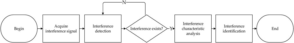
FIGURE 1. The interference detection and recognition process.

In fact, in the process of interference detection, faced with different types of interference, the detection effect is also vastly different. Therefore, different interference detection algorithms are often designed in the face of different interferences. Therefore, the division of interference detection and recognition technologies is not obvious. Interference detection has been widely considered and has relatively complete theory and research. Interference recognition has been developed in recent years and is briefly introduced at the end of this section.

2.1 Classification of interference

Due to the functionality of satellite navigation systems, different from other radio systems, it is necessary to consider intentional interference. The types of navigation signal interference mainly include blanket interference and spoofing interference [26]. Compound interference, a combination of blanket interference and spoofing interference, is also common. Generally, in the GNSS domain, jamming refers to intentional suppression interference, and spoofing refers to intentional deception interference. Blanket interference can be interpreted as radio frequency interference (RFI). Its purpose is to suppress the navigation signal from the time domain or frequency domain using a high-power interference signal to prevent a navigation receiver from working normally [27]. The RFI usually referred to may be unintentional interference in the electromagnetic environment. Spoofing refers to the use of signals similar to navigation signals as interference signals to affect satellite navigation receivers, thereby causing the navigation system to deviate from the correct positioning and navigation and provide incorrect navigation information. Since satellite navigation systems are also used for timing services, there is also deception in the timing services [28]. On the other hand, a multipath interference signal in a satellite navigation system is very similar to a real signal, but multipath interference is the unintended interference caused by different signal paths [29]. Spoofing interference is usually intentional.

Blanket interference is simple in principle, easy to implement, low in cost, and obvious in effect. Most existing interference is blanket interference. Generally, the higher the power of the interference signal is, the better the interference effects.

Blanket interference can be distinguished into two types in terms of the frequency domain: narrowband interference and broadband interference. Narrowband interference, whose frequency is concentrated in a small bandwidth, has strong pertinence. Partial band interference or targeting interference also expresses a similar meaning [30]. The most common narrowband interference is Gaussian narrowband interference, which is generated by passing white Gaussian noise through a filter. Another common narrowband interference is tone interference, that is, an interference signal only at a single frequency point, single-tone interference or an interference signal at several frequency points, and multitone interference [31]. For wideband interference, the bandwidth of the interference signal is wide. Blocking interference has a similar meaning [32]. The most common wideband interference is Gaussian wideband interference, which has a wide bandwidth. Another common broadband interference is frequency modulation interference (also known as sweeping interference) [33]. The frequency of the interference signal varies over a wide range, and is typically linear frequency modulation interference (LFM) [34]. Chirp interference means the same thing. In terms of generation mode, random binary codes can be modulated to the interference frequency band in BPSK mode to form narrowband BPSK interference or wideband BPSK interference. They are also called spread spectrum interference or matched spectrum interference [35]. The frequency spectra of common blanket interference types are shown in Figure 2.

FIGURE 2

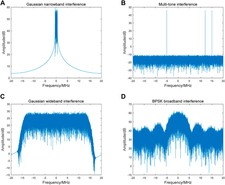
FIGURE 2. The frequency spectra of common blanket interference types: (A) Gaussian narrowband interference; (B) multitone interference; (C) Gaussian broadband interference (D) BPSK broadband interference.

In terms of the time domain, blanket interference can be divided into pulse interference and continuous wave interference (CWI). Pulse interference refers to the interference that focuses the interference energy on a certain period of time in a pulse cycle to transmit [36]. The opposite of pulse interference is continuous wave interference, which has a longer duration [37]. Because of the cost, pulse interference with a short duration is usually high-power broadband interference, while continuous wave interference is mostly narrowband interference. However, this is not absolute. For better interference effects, broadband interference can also be used in the form of continuous wave interference. The classification of blanket interference is shown in Figure 3.

FIGURE 3

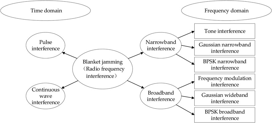
FIGURE 3. Classification of blanket interference (RFI).

A spoofing interference signal is similar to a real signal in form, and its purpose is not only to make a target receiver lose its original working performance but also to make it operate in a specified way [38]. In the field of satellite navigation, spoofing interference can make the target positioning be offset or be unable to complete the positioning and can make the target positioning to its specified position, which makes the harm of spoofing interference significant.

Spoofing interference in the field of satellite navigation can be generally divided into two categories, namely, generative spoofing interference and repeater spoofing interference. Generative spoofing interference equipment is mainly composed of a signal analog source, power amplifiers, and transmit antennas. Since the civil signal structure, signal characteristics, pseudocode characteristics and navigation message structure of existing navigation systems are all public, generative spoofing is easy to generate by imitating a real signal [39]. After receiving a real navigation signal, repeater spoofing will delay and amplify the power of the signal. Although the specific structure of the real navigation signal is not known, it can still have a certain impact on the positioning result [40]. Repeater spoofing is more commonly used in the military field. The military pseudocode of a navigation system is secret, so generating generative spoofing is almost impossible. Based on these two basic spoofing interference generation methods, spoofing interference continues to develop new methods, such as complex spoofing interference generated according to the estimated information after receiving the real signal or spoofing interference forwarded by using multiple antennas. Spoofing is sometimes divided into simple spoofing and complex spoofing according to their different functions.

2.2 Detection theory

One of the theoretical bases of interference detection technology is detection theory, which is used to determine whether a signal exists, that is, whether there is a signal or only noise in the case of noise [41]. Let $s\left[n\right]$ denote a signal and $w\left[n\right]$ denote noise; then, we can express it as the following two hypotheses:

$\begin{array}{cc}{H}_0:x\left[n\right]=w\left[n\right]& n=\mathrm{0,1},...,N-1\\ H_1:x\left[n\right]=s\left[n\right]+w\left[n\right]& n=\mathrm{0,1},...,N-1\end{array}(1)$

In mathematics, if $H_0$ is true and we think $H_1$ is true, it is called a type I error. If $H_1$ is true and we think $H_0$ is true, it is called a type II error. In detection theory, the first type of error can be regarded as a misjudgment that there is a signal when there is no signal. Therefore, this event can also be called a false alarm (FA), and the probability of the occurrence of a false alarm is called the false alarm probability, which is usually denoted by $P_{FA}$. If $H_1$ is true, and we think $H_1$ is true, we can consider that we have successfully detected a signal. This event is called detection, and the probability of successful detection is called the detection probability, which is usually denoted by $P_D$. In statistics, the detection probability is also called the power of the test.

For each value of $\mathit{x}$, the ratio of the probability of $H_1$ to the probability of $H_0$ is called the likelihood ratio $L\left(\mathit{x}\right)$, where $\mathit{x}=\left[\begin{array}{cccc}x\left[0\right]& x\left[1\right]& \cdots & x\left[N-1\right]\end{array}\right]$. If we consider that the likelihood ratio is greater than a certain threshold, that is, the ratio of the probability of $H_1$ to the probability of $H_0$ is greater than a certain threshold $\gamma$,

$L\left(\mathbf{x}\right)=\frac{p\left(\mathbf{x};H_1\right)}{p\left(\mathbf{x};H_0\right)}>\gamma (2)$

You can say that event $H_1$ happened. This test is called the likelihood ratio test (LRT). If $p\left(\mathit{x};H_1\right)$; $p\left(\mathit{x};H_1\right)$ are known and the false alarm probability $P_{FA}=\alpha$ is set, the threshold $\gamma$ can be obtained using the Neyman-Pearson theorem (NP theorem),

$p_{FA}={\int }_{\left\{\mathbf{x}:L\left(\mathbf{x}\right)>\gamma \right\}}p\left(\mathbf{x};H_0\right)d\mathbf{x}=\alpha (3)$

The false alarm probability is usually a very small value, also known as the significance level or detection scale in statistics, which indicates that the NP theorem seeks the decision with the maximum detection probability when limiting the false alarm probability to a small value. It aims to protect hypothesis $H_0$ and not accept hypothesis $H_1$ easily. In some practical applications, once a signal is detected, it is necessary to make a response, which requires paying a certain price. If the false alarm probability is too large, it will cause unacceptable losses. If no signal is detected, no action is needed. If the cost caused by not detecting the signal is large, the NP theorem is not necessarily applicable, and some adjustment is needed.

For example, in the case of deterministic signals, if signal $s\left[n\right]$ is known and noise $w\left[n\right]$ is white Gaussian noise with variance ${\sigma }^2$, the specific probability density function can be substituted into Eq. 2 and simplified to obtain:

$T\left(\mathbf{x}\right)={\displaystyle \sum }_{n=0}^{N-1}x\left[n\right]s\left[n\right]>{\gamma }^{\prime }(4)$

The right side of the inequality is denoted by a new threshold ${\gamma }^{\prime }$. The left side of the inequality $T\left(\mathit{x}\right)$ is called the test statistic, which is actually the cross-correlation between the known signal and the actual observed value. This is the NP detector, which consists of a test statistic $T\left(\mathit{x}\right)$ and a threshold ${\gamma }^{\prime }$. The threshold is also obtained by the NP theorem. The NP detector at this time is also called the matched detector.

If the signal is a random signal, assume that it is a Gaussian random process with variance ${\sigma }_s^2$; then,

$T\left(\mathbf{x}\right)={\displaystyle \sum }_{n=0}^{N-1}{x}^2\left[n\right]>{\gamma }^{″}(5)$

Here, the test statistic $T\left(\mathit{x}\right)$ is the energy of the observed data, and the NP detector at this time is also called the energy detector. A matched filter and energy detector are basic and common detection methods.

2.3 Detection of blanket interference

In a satellite navigation system, a common signal model is

$x\left(i\right)=s\left(i\right)+j\left(i\right)+n\left(i\right)(6)$

This means satellite navigation signal, jamming and noise. The noise is not always white Gaussian noise, so it is directly denoted as $n\left(i\right)$. From energy detection, blanket interference detection technology mainly includes energy detection in the time domain and the frequency domain. Energy detection in the frequency domain is based on the fast Fourier transform (FFT). A time-frequency plane detection method based on a short-time Fourier transform (STFT) is also developing rapidly.

There have been some developments in blanket interference detection based on energy detection. The same detector has different detection performances for different interference types. Some detectors have good detection effects for specific interference. Based on energy detection, some algorithms improve the detection performance of some particular disturbances. Nunes F. D. et al. proposed blind interference detection based on fourth-order cumulants, which is more suitable for FM interference. Compared with the kurtosis algorithm, although the computational amount is increased, it achieves better performance [42]. Huo S. et al. improved the consecutive mean excision (CME) algorithm and proposed a block-flow method based on the backward CME (BCME) algorithm. This method can reduce the amount of storage and computation under the condition that the performance of monitoring pulse interference is similar [43].

Another rapidly developing direction is interference detection algorithms based on time-frequency analysis technology. Sun K. et al. proposed a new reassigned spectrogram method for interference detection for GNSS receivers. It has good detection performance for LFM interference [44]. They also provide another class of interference detection algorithms, aiming to transform the time scale using a wavelet transform, which can be used to detect weak RF signals. A new STFT method based on time-frequency domain analysis proposed by Wang P. improves the performance of narrowband and broadband detection in a signal with a low dry-to-noise ratio [45]. Lv Q. et al. also provided a time-frequency domain-based detection method using a goodness-of-fit (GoF) test [46]. Compared with the Hough transform of the Wigner-Ville distribution, the reassigned smoothed pseudo Wigner-Ville distribution (RSPWVD) has better performance in reducing cross-term interference and requires less computation [47].

Other interference detection algorithms are also feasible. Motella B. et al. applied detection theory to the field of satellite navigation and used a goodness-of-fit method to detect interference in satellite navigation systems [48]. Wu Q. proposed an interference detection algorithm for GNSS receivers based on adaptive subspace tracking technology and receiver autonomous integrity monitoring (RAIM) [49]. Zhai S. proposed an interference detection algorithm based on fuzzy logic fusion. In particular, for the problem of reduced detection performance caused by noise fluctuations in a complex electromagnetic environment, the proposed algorithm introduces the idea of fuzzy logic [50]. Silva F. B. et al. proposed a new precorrelation interference detection technology based on non-negative matrix factorization (NMF). The proposed technology uses NMF to extract the time and frequency properties of a received signal from its spectrogram. The estimated spectral shape is then compared with the time slices of the spectrogram using a similarity function to detect the presence of RFI [51].

2.4 Detection of spoofing interference

Spoofing interference detection technology is quite complex, and the classification methods are different. This paper simply divides spoofing interference detection technology into signal categories and other categories.

Methods in signal categories are mainly related to the characteristics of the signal itself. The power of spoofing interference is usually larger than the real signal power, so it can be detected using the signal strength. The common detection method is absolute power monitoring [52]. A method comparing the power of the L1 channel and L2 channel is called relative power detection. It is also effective in detecting the carrier-to-noise ratio (CNR) of the signal [53]. Among these methods, a special method is auto gain control (AGC) detection. AGC detection is located at the RF front end of a receiver before the correlation operation. The principle is that the AGC at the RF front end of the receiver will produce large fluctuations when spoofing interference exists [54]. Because spoofing interference is forwarded, the arrival angle of the signal is different from that of the real signal. Therefore, spoofing interference can also be detected from the arrival angle of the signal [55]. Magiera J. combined array signal processing to detect spoofing interference according to the difference between the arrival angle of the spoofing signal and that of the real signal and used beamforming for spoofing interference mitigation [56]. The repeater spoofing interference has a delay, so it can also be detected by the arrival time [57]. Carrier Doppler can also be used for spoofing interference detection. This method compares the Doppler shift change of the real signal with the Doppler shift change calculated from the reported position [58]. Signal quality monitoring (SQM) is a very common detection method that mainly uses the output of the correlator. When there is spoofing interference, the related summit will be distorted [59]. Wang W. et al. proposed a detection method based on the S-curve bias (SCB) [60]. This algorithm works well and is expected to be combined with other algorithms. Multi-peak detection can also be classified into this category [61]. There are also methods such as residual signal detection and carrier phase detection, but their principles are mostly the same.

Different from the methods in signal categories, methods in other categories detect spoofing signals from aspects such as data layer and positioning results. At the data layer, navigation messages can be encrypted, which is useful for detecting spoofing interference. Lewis S. W. et al. presented a GNSS interferometric reflectometry (GNSS-IR) signature-based method [62]. Humphreys T. E. demonstrated that navigation message authentication (NMA) is effective for anti-spoofing [63]. Receiver autonomous integrity monitoring (RAIM) methods can detect repeater spoofing interference. For repeater spoofing, the repeater spoofing signal increases the satellite delay, so the calculated pseudorange value will mutate after the receiver receives the repeater spoofing signal, causing the consistency of the calculated pseudorange value of each satellite to worsen. Han S. et al. combined particle filtering and the RAIM algorithm, which can effectively deal with the spoofing interference of multiple satellites [64]. By comparing the positioning results of the satellite navigation system with the positioning results based on other methods, we can judge whether the satellite navigation system receives spoofing interference. Khanafseh S. et al. used the results of an inertial navigation system (INS) combined with RAIM to detect spoofing signals [65]. Jeong S. et al. proposed a method to detect spoofing interference, which uses the GNSS augmentation system as the correction data [66]. Spoofing interference detection can be combined with machine learning. Shafiee E. al. extracted the early-late phase, delta, and signal level as the three main features from the correlation output of the tracking loop. Using these features, spoofing detection can be performed by exploiting conventional machine learning algorithms such as K-nearest neighbor (KNN) and naive Bayesian classifiers [67]. Li J. et al. proposed a GNSS anti-spoofing method based on the idea of confrontation evolution of a general adverse network (GAN) [68].

2.5 Interference recognition

The recognition of spoofing interference can be regarded as distinguishing the real signal and spoofing interference in the received signal, and then the effective part of the received signal can be used to continue the localization instead of using the spoofing interference signal for the subsequent localization solution. To a certain extent, the detection of spoofing interference basically completes the suppression of spoofing interference. The research in this direction mainly involves the suppression of spoofing interference, so we will not introduce it. The recognition of blanket interference is similar to the detection of blanket interference. The characteristics of the interference signal can be extracted from the time domain, the frequency domain and the time-frequency domain. By analyzing the characteristics of the blanket interference, the types of blanket interference can be identified effectively, and the corresponding filters can be designed to suppress the blanket interference.

Most interference recognition is based on pattern recognition [69] and machine learning [70] theory, although there are other ways. In the field of radar, the application of machine learning algorithms is more common. In the field of GNSS, research on interference recognition is limited. Kang C. et al. proposed a time-domain identification method based on an adaptive cascading IIR notch filter to identify single-tone, multitone, swept continuous wave interference (CWI) and band-limited white Gaussian noise (BLWN) [71]. Ferre R. M. proposed applying machine learning approaches to sort the interference signal into five classes [72]. Chen X. et al. proposed a deep convolutional neural network (DNN) named FPS-DNN on the basis of a convolutional neural network (CNN) for fingerprint recognition. This method can classify the interference types very well [73].

2.6 Brief summary

Interference detection technology is divided into blanket interference detection technology and spoofing interference detection technology. The development of blanket interference detection technology is relatively perfect. Blanket interference detection starts from energy detection and accumulates the sum in different transform domains, such as the time domain, frequency domain, time-frequency domain, and wavelet domain, to detect interference signals. According to the characteristics of interference signals, different detection algorithms have different effects. With the complexity and change of the interference signal, the targeted algorithm can often achieve better results. The detection technology of spoofing is quite complex, and the classification methods are different. In this paper, spoofing detection technology is simply divided into a signal class and other classes. Spoofing interference detection from the signal level involves signal processing technology, and the signal power and signal correlation peak are monitored. From the information level, we can verify whether the obtained information is wrong. We can use inertial navigation, data encryption and other methods to verify the positioning results and navigation messages. These two aspects involve different technologies, but both can play a role in spoofing detection, and their development is relatively independent.

Interference recognition technology classifies interference signals by extracting their features. The classification methods rely on pattern recognition techniques that emerged in the 1960s and 1970s, including support vector machines, clustering, principal component analysis and so on. In the 1980s, machine learning became an independent subject field and developed rapidly, and various machine learning techniques appeared. With the rise of machine learning, its functionality is almost perfect to replace the pattern recognition methods of the past. Interference recognition technology has developed rapidly on this basis.

3 Interference source direction finding

Interference source direction finding technology, or interference source orientation technology, determines the direction of the coming interference signal. The interference signal and the real signal arrive in different directions, so the interference source direction finding method can be used to detect whether the interference signal exists. The interference source direction finding method can also be used to calculate the interference source location based on the angle information. Some interference direction finding technology is not stated separately but as a part of interference detection or localization. However, with the development of spatial spectrum estimation, the extensive use of array antennas [74], spatial filtering [75], adaptive beamforming and anti-interference [76], it is enough to be a separate category of technology worth discussing.

To measure the direction of signal arrival, there are usually three main methods: amplitude direction finding, phase direction finding, and spatial spectrum estimation direction finding. Interference source direction finding technology can also be divided into scalar direction finding and vector direction finding. The amplitude method and phase method are traditional scalar direction methods, while the spatial spectrum estimation method is a vector direction method. This section focuses on the basic principles of spatial spectrum estimation methods and the latest advances in their technology but also briefly mentions the related research on amplitude direction finding and phase direction finding.

3.1 Amplitude direction finding

Among amplitude direction finding methods, the most common method is the comparative amplitude direction finding method. By comparing the amplitude of the signals received by antennas at different positions, the angle information of the signals can be calculated. Typical direction finding systems include four-antenna array Adcock direction finding [77] and Watson-Watt direction finding [78]. An Adcock direction finding system is based on a four-antenna array [79], which calculates the direction of the signal based on the amplitude of the signal received by the north‒south and west‒east antennas [80]. A dual-channel Watson-Watt direction finding system requires two receiving channels with exactly the same amplitude and phase responses [81]. There are also single-channel Watson-Watt direction finding systems.

There are also some traditional amplitude methods, such as the maximum signal amplitude method, which uses a strong directional antenna to directly take the direction of the maximum signal amplitude as the direction of the incoming wave. Alternatively, the minimum signal method uses a figure-8 antenna to receive the signal, with the zero point of the antenna pattern being the direction of the incoming wave [82]. These methods are simple, but the direction finding error is large.

3.2 Phase direction finding

Phase direction finding methods are mainly based on interferometers. One is a phase interferometer. It estimates the angle information of the incoming wave through the phase difference between the signals received by the antennas at different positions [83]. A phase interferometer can realize the direction finding of a single pulse, so it is also called phase single pulse direction finding. The other type of interferometer, a correlative interferometer, estimates the direction of the signal by comparing the measured phase difference distribution with the one that has been stored beforehand. The direction corresponding to the maximum of the correlation coefficient is the direction of the signal [84]. The direction finding accuracy of interferometers often depends on the baseline, and multibaseline interferometers are mainly used in practical applications.

In addition, there are some other phase direction finding methods, such as Doppler direction finding based on the Doppler characteristics of the signal [85]. A Wullenweber direction finding system, which is one of the older methods, uses a circular array of antennas [86]. A system that uses the array antenna and the time difference of arrival to find the direction is also a phase direction finding method in essence.

3.3 Spatial spectrum estimation direction finding

Spatial spectral estimation direction finding has superresolution capability, also known as superresolution direction finding. Compared with traditional methods, a spatial spectrum estimation direction finding method is more accurate and widely used and has been developed rapidly in recent years. Spatial spectrum estimation direction finding is developed on the basis of array signal processing and spectrum estimation. It uses array antennas to receive signals, estimate the spatial spectrum of signals, and estimate the direction information of signals. Similar to the frequency spectrum, the spatial spectrum only takes the direction in space as the abscissa, reflecting the direction information of the signal. The diagram of an array antenna is shown in Figure 4.

FIGURE 4

FIGURE 4. Diagram of an array antenna.

Among spatial spectrum estimation methods, the most typical algorithm is multiple signal classification (MUSIC) [87]. MUSIC estimates the power spectrum of a signal by decomposing it into a signal subspace and a noise subspace. In array signal processing, MUSIC is used to estimate the spatial spectrum of a signal.

The observed data are regarded as the sum of the signal and noise,

$x\left(t\right)=s\left(t\right)+w\left(t\right)(7)$

The wave surface of a signal needs to travel $d\mathit{cos}\theta$ more distance to reach array element 1 than to reach array element 2, so the time to receive the signal at array element 1 will be later than that at array element 2. This time interval is

${\tau }_0=\frac{d\cos \theta }{c}=\frac{d\cos \theta }{\lambda f}(8)$

where $c$ represents the speed of light, $\lambda$ represents the wavelength of the signal, and $f$ represents the frequency of the signal. For the exponential signal, this delay can be expressed as the difference in phase, i.e.,

$s\left(t-{\tau }_0\right)=s\left(t\right)e^{-j\omega {\tau }_0}=s\left(t\right)e^{-j\omega \frac{d\cos \theta }{\lambda f}}=s\left(t\right)e^{-j\frac{2\pi }{\lambda }d\cos \theta }(9)$

Assuming that the number of array elements is $N$ and $x_i\left(t\right)$ is used to represent the observed signal of the $i$ th array element, the received signal of the array can be expressed as:

$\left[\begin{array}{c}{x}_1\left(t\right)\\ x_2\left(t\right)\\ ⋮\\ x_N\left(t\right)\end{array}\right]=\left[\begin{array}{c}1\\ e^{-j\frac{2\pi }{\lambda }d\cos \theta }\\ ⋮\\ e^{-j\frac{2\pi }{\lambda }\left(N-1\right)d\cos \theta }\end{array}\right]s\left(t\right)+\left[\begin{array}{c}{w}_1\left(t\right)\\ w_2\left(t\right)\\ ⋮\\ w_N\left(t\right)\end{array}\right](10)$

For multiple signal sources, assume that the number of signal sources is $D$, let $s_i\left(t\right)$ denote the signal transmitted by the $i$ th signal source, and let ${\theta }_i$ denote the incident angle of the signal. In this case, Equation 10 is extended as follows:

$\left[\begin{array}{c}{x}_1\left(t\right)\\ x_2\left(t\right)\\ ⋮\\ x_N\left(t\right)\end{array}\right]=\left[\begin{array}{cccc}1& 1& \cdots & 1\\ e^{-j\frac{2\pi }{\lambda }d\cos {\theta }_1}& e^{-j\frac{2\pi }{\lambda }d\cos {\theta }_2}& \cdots & e^{-j\frac{2\pi }{\lambda }d\cos {\theta }_D}\\ ⋮& ⋮& \ddots & ⋮\\ e^{-j\frac{2\pi }{\lambda }\left(N-1\right)d\cos {\theta }_1}& e^{-j\frac{2\pi }{\lambda }\left(N-1\right)d\cos {\theta }_2}& \cdots & e^{-j\frac{2\pi }{\lambda }\left(N-1\right)d\cos {\theta }_D}\end{array}\right]\left[\begin{array}{c}{s}_1\left(t\right)\\ s_2\left(t\right)\\ ⋮\\ s_D\left(t\right)\end{array}\right]+\left[\begin{array}{c}{w}_1\left(t\right)\\ w_2\left(t\right)\\ ⋮\\ w_N\left(t\right)\end{array}\right](11)$

Define the vector $\mathit{x}={\left[\begin{array}{cccc}{x}_1\left(t\right)& x_2\left(t\right)& \cdots & x_N\left(t\right)\end{array}\right]}^T$, which represents a data vector of observations and is a vector of $N\times 1$ dimension;

vector $\mathit{S}={\left[\begin{array}{cccc}{s}_1\left(t\right)& s_2\left(t\right)& \cdots & s_D\left(t\right)\end{array}\right]}^T$ represents the signal source vector, which is a vector of $D\times 1$ dimension;

vector $\mathit{w}={\left[\begin{array}{cccc}{w}_1\left(t\right)& w_2\left(t\right)& \cdots & w_N\left(t\right)\end{array}\right]}^T$ represents the noise vector, which is a vector of $N\times 1$ dimension;

vector $\mathit{a}\left({\theta }_i\right)={\left[\begin{array}{cccc}1& e^{-j\frac{2\pi }{\lambda }d\mathit{cos}{\theta }_i}& \cdots & e^{-j\frac{2\pi }{\lambda }\left(N-1\right)d\mathit{cos}{\theta }_i}\end{array}\right]}^T$, called the steering vector, is a vector of $N\times 1$ dimension;

matrix $\mathit{A}=\left[\begin{array}{cccc}\mathit{a}\left({\theta }_1\right)& \mathit{a}\left({\theta }_2\right)& \cdots & \mathit{a}\left({\theta }_D\right)\end{array}\right]$ represents the direction matrix, which is a matrix of $N\times D$ dimensions;

$\mathit{s}$ denotes the signal vector received by the array antenna, $\mathit{s}=\mathit{A}\cdot \mathit{S}$. Therefore, Eq. 11 can be expressed as

$\mathbf{x}=\mathbf{s}+\mathbf{w}=\mathbf{A}\cdot \mathbf{S}+\mathbf{w}(12)$

Since noise and signal are not correlated, the autocorrelation ${\mathit{R}}_{\mathit{x}}$ of the observed data can be expressed as the sum of the autocorrelation of the signal received by the array antenna and the noise autocorrelation

${\mathbf{R}}_{\mathbf{x}}={\mathbf{R}}_{\mathbf{s}}+{\mathbf{R}}_{\mathbf{w}}=\left(\mathbf{A}\mathbf{S}\right){\left(\mathbf{A}\mathbf{S}\right)}^H+{\sigma }_w^2\mathbf{I}=\mathbf{A}{\mathbf{R}}_{\mathbf{S}}{\mathbf{A}}^H+{\sigma }_w^2\mathbf{I}(13)$

After eigenvalue decomposition,

${\mathbf{R}}_{\mathbf{x}}={\mathbf{R}}_{\mathbf{s}}+{\mathbf{R}}_{\mathbf{w}}={\displaystyle \sum }_{i=1}^N{\lambda }_s{e}_s{e}_s^H+{\displaystyle \sum }_{i=1}^N{\lambda }_w{e}_w{e}_w^H=U_s{\mathrm{\Sigma }}_s{U}_s^H+U_w{\mathrm{\Sigma }}_w{U}_w^H(14)$

${\mathit{R}}_{\mathit{S}}=\mathit{S}{\mathit{S}}^H=diag\left[\begin{array}{cccc}{P}_1& P_2& \cdots & P_D\end{array}\right]$ is a diagonal array, and the diagonal element $P_i$ is actually the signal power of the signal source. At this time, the autocorrelation ${\mathit{R}}_{\mathit{s}}$ of the signal just conforms to the definition of eigenvalue decomposition, which indicates that among the $N$ eigenvalues of the autocorrelation ${\mathit{R}}_{\mathit{s}}$ of the signal, only $D$ are non-zero values, which are the signal power of the signal source.

${\mathbf{R}}_{\mathbf{s}}=\mathbf{A}{\mathbf{R}}_{\mathbf{S}}{\mathbf{A}}^H={\displaystyle \sum }_{i=1}^D{P}_i\mathbf{a}\left({\theta }_i\right){\mathbf{a}}^H\left({\theta }_i\right)(15)$

Thus, the eigenvalues and eigenvectors of the autocorrelation matrix ${\mathit{R}}_{\mathit{x}}$ of the observed data are calculated. For $D$ signal sources,

${\lambda }_1\ge {\lambda }_2\ge \cdots \ge {\lambda }_D\ge {\lambda }_{D+1}=\cdots {\lambda }_M={\sigma }_w^2(16)$

The eigenvectors corresponding to the first $D$ eigenvalues, called principal eigenvectors, constitute the signal subspace. The eigenvectors corresponding to the last $N-D$ eigenvalues constitute the noise subspace. Assuming that the signal-to-noise ratio (SNR) of the received signal is very high and contains almost no noise, we can approximate ${\sigma }_w^2=0$. Because eigenvectors with different eigenvalues are orthogonal to each other, the signal subspace is orthogonal to the noise subspace.

$a^H\left(\theta \right)U_N=0(17)$

The MUSIC spectrum is defined as

$P_{MUSIC}=\frac{1}{a^H\left(\theta \right)U_N{U}_N^{H}a\left(\theta \right)}(18)$

If the signal does not contain noise, the denominator is zero, and the MUSIC spectrum is meaningless, so the MUSIC spectrum is also called the MUSIC pseudospectrum. However, in fact, noise is always there, and it is just approximately zero. By taking the inverse, we can obtain the peak, which is the estimate of the angle of the signal.

The number of interference sources is set as 3, and the arrival directions of the interference signals are $-30^{\circ }$, $0^{\circ }$, and $60^{\circ }$. Select the linear array element, the number of array elements is 8, and the number of fast beats is 500. The MUSIC spatial spectrum estimation is carried out in the cases of SNRs of 10 and 1. As seen from the simulation results, when the SNR is high, the MUSIC algorithm can simultaneously identify the interference signals in three directions and provide relatively accurate direction information, as shown in Figure 5A. When the SNR decreases, the performance of the MUSIC algorithm is affected when the simulation is carried out under the same three interference sources, as shown in Figure 5B.

FIGURE 5

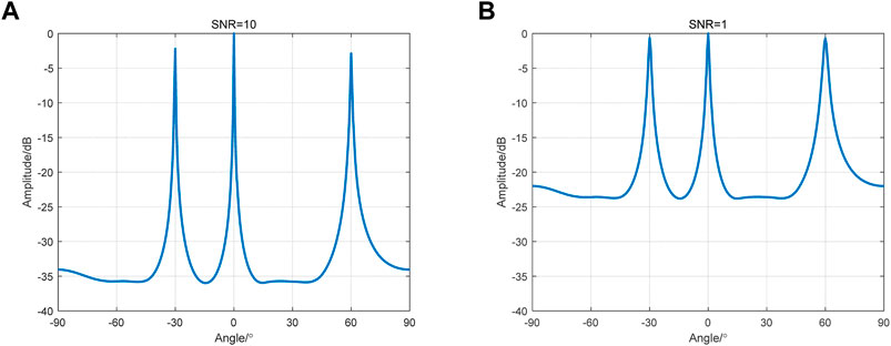
FIGURE 5. Simulation results of the MUSIC algorithm. (A) The result of direction finding when the SNR is 10. (B) The result of direction finding when the SNR is 1.

In 1969, Capon proposed the minimum variance spectrum estimation method (MVM), and to some extent, spatial spectrum estimation was developed on this basis [88].

In 1979, Schmidt R. proposed the MUSIC algorithm, whose basic idea is to divide the received signal into an orthogonal signal subspace and a noise subspace. The performance of the method is close to that of the maximum likelihood method, but the computational amount is enormous. This is a landmark achievement of spatial spectrum estimation theory. In 1986, Roy R. et al. proposed the ESPRIT algorithm, the core of which is to rely on the rotational invariance of the signal subspace and use the least square method to obtain the angle of arrival. The search process of the spectral peak in the MUSIC algorithm is avoided, and the calculation amount is effectively reduced. This method not only has good resolution but also obtains high real-time performance [89].

In the late 1980s, angle estimation algorithms for subspace fitting emerged. This kind of method obtains the desired objective function by deducing and constructing a fitting relation, so the fitting model determines the accuracy of the algorithm. Typical algorithms include the maximum likelihood (ML) algorithm [90], the weighted subspace fitting (WSF) algorithm [91], and the multidimensional MUSIC (MD-MUSIC) algorithm [92]. The performance of this kind of algorithm is better, and the requirement of SNR is reduced to some extent, but the computational amount is large.

In 1995, Marcos S. et al. proposed the propagator method (PM) algorithm, which avoided the covariance matrix decomposition of the received signals of the array. Although compared with the MUSIC algorithm, the performance of partial resolution was lost, the computational amount was greatly reduced [93].

The development in recent years mainly has the following aspects. First, it is no longer satisfied with the use of second-order statistics (SOS) but with the use of high-order cumulants [94]. Common algorithms are usually based on fourth-order cumulants (FOCs) [95]. The second is compressed sensing (CS) [96], which breaks through the bandwidth limitation of traditional sampling theory and uses far less measured data than Nyquist sampling data, making superresolution signal processing possible. The theory of compressed sensing can greatly reduce the number of antenna elements and sampled data to reduce the amount of signal processing data. Therefore, the application of CS in direction estimation is increasingly widespread [97]. Deep learning is a development of machine learning. It has also been introduced into the research of direction finding technology. Deep neural networks have stronger representation and learning ability, so they can obtain better direction finding performance than traditional neural networks [98].

3.4 Brief summary

The principle of amplitude methods is simple and easy to implement, but the precision is not good. Since the interference to the satellite signals is often attached to the carrier frequency, the wavelength of the interference signals is short, and the phase information is obvious. Therefore, phase methods, such as interferometer direction finding, have higher measurement accuracy than the previous amplitude method. Based on the theory of array signal processing and spatial spectrum estimation, the direction finding of multiple interference sources can be realized simultaneously. This makes the array antennas and spatial spectrum estimation more widely used in practice. Spatial spectrum estimation methods have high measurement accuracy, breaking the Rayleigh limit, and have the ability of super resolution direction finding. However, the algorithm has a high SNR requirement and a large amount of calculation, so it is difficult to carry out real-time processing. Compared with the amplitude method, the phase method improves the sensitivity, but the number of interference sources that can be measured is limited. The spatial spectrum method further improves the sensitivity based on the phase method. It can measure multiple interference sources at the same time, but the number of interference sources cannot be more than the number of array elements.

4 Interference source location and tracking

Interference source location is the ultimate goal of interference monitoring. Once the location of the interference source is determined, appropriate algorithms can be used to suppress the noise. The user can also choose to stay away from the interference source or destroy it. The location of the interference source can be said to be the most important part of interference monitoring. The algorithms of interference source location are mainly based on four kinds of algorithms and their joint algorithms. They are received signal strength (RSS), time difference of arrival (TDOA), frequency difference of arrival (FDOA), angle of arrival (AOA) or direction of arrival (DOA) [99]. These algorithms set up a set of equations through the signal strength information, time information, frequency information and angle information of the interference signal and then solved the three-dimensional coordinates of the interference source. These algorithms are widely used in passive location, sound source location, cooperative location and indoor location [100]. The classification of interference source location is also mature and generally uses the classification method described in this paper.

4.1 Received signal strength (RSS)

From the received signal strength, a path loss model can be used to infer the distance between the monitoring point and the interference source [101]. Then, a system of equations can be established to find the location of the interference source through the observation data of multiple nodes.

$RS{S}_i=P_0-10n{\log }_{10}\left(\frac{d_i}{d_0}\right)+{\sigma }_i(19)$

where $P_0$ is the received power from the transmitter to the reference distance $d_0$ and $P_0$ and $d_0$ are known. $n$ and ${\sigma }_i$ require actual measurements of the environment to be roughly determined. Small errors in RSS measurements can lead to large position errors. Even simple ground reflections can seriously affect accuracy. Even if the path model is optimized, its positioning accuracy is poor. One improvement of the RSS is the difference in the RSS (DRSS).

$DRS{S}_{i-j}=RS{S}_i-RS{S}_j(20)$

Thompson, R. J. R. et al. used an RSS method to locate RF interference sources in the GPS L1 band and considered the effect of ground refraction [102]. Wang, P. et al. proposed a simple and computationally efficient GNSS RFI localization technique based on DRSS measurements from crowdsourced devices. In this method, the weighted centroid of receiver position estimation is used as the RFI position estimation, which reduces the computational amount [103].

4.2 Time difference of arrival (TDOA)

The TDOA evolved from the time of arrival (TOA). The principle of the TOA algorithm is similar to that of the GNSS. By measuring the arrival time of the signal transmission process from the unknown position point to the known position point, the distance from the unknown point to the known point is calculated. Then, enumerate the equation to solve the coordinates of the unknown point.

Let $t_i$ denote the observed time at the $i$ th known point and $t$ denote the observed time at the unknown point. $\tau$ is used to represent the time error caused by a series of processes such as modulation and demodulation. Sometimes, this term can also be expressed as white Gaussian noise. Then, the distance from the unknown point to the $i$ known point is

$d_i=c\left(t_i-t\right)+c\tau (21)$

Let $\left(x_i,y_i,z_i\right)$ denote the coordinates of the known point and $\left(x,y,z\right)$ denote the coordinates of the unknown point; then, the distance from the unknown point to the known point can also be expressed as

$d_i=c\left(t_i-t\right)+\mathrm{c}\tau =\sqrt{{\left(x_i-x\right)}^2+{\left(y_i-y\right)}^2+{\left(z_i-z\right)}^2}(22)$

The observation data of multiple nodes are used to establish the equation, and then the unknown position of the three-dimensional coordinates can be solved. It is worth noting that the TOA method used for interference source location is not applicable. The TOA algorithm requires highly accurate clock synchronization between the point to be measured and the known point. In the process of monitoring interference, whether intentional or unintentional interference, it is naturally impossible to expect the interference signal to cooperate, and there is no synchronization on the clock. The TOA algorithm is introduced as a passive positioning algorithm, which is generally used in indoor positioning [104].

Select a primary node $\left(x_0,y_0,z_0\right)$. Its distance from the unknown point is $d_0$. Then, the distance difference $\Delta d_i$ between different nodes and the unknown point can be expressed as

$\Delta d_i=d_0-d_i=c\left(t_i-t_0\right)+c\tau (23)$

This is how the TDOA algorithm works. The TDOA algorithm calculates the distance difference between the unknown point and the known position point by measuring the difference between the arrival time of the signal transmitted by the unknown point and multiple known points. The TDOA algorithm still requires highly accurate clock synchronization between known measurement points, but unlike the TOA algorithm, the TDOA algorithm no longer requires the time information of unknown measurement points. This enables the TDOA algorithm to be used to locate interference sources. Common solutions of the TDOA algorithm are as follows: the Chan algorithm [105], Taylor series method [106], and weighted least squares method [107].

A common TDOA modification is the asynchronous time difference of arrival (A-TDOA). Díez-González J. et al. optimized the A-TDOA algorithm to allow higher refresh rates of localization signals and provide higher accuracy in the A-TDOA architecture [108]. Another improved method is the sparse time difference of arrival (S-TDOA). Uysal C. used sparse sensor data to estimate the TDOA, which reduced the computational amount. This method is more suitable for low SNR signals [109]. The particle swarm optimization (POS) algorithm is widely used to solve non-linear optimization problems, so it is often used to solve the TDOA equation [110].

4.3 Frequency difference of arrival (FDOA)

The FDOA makes use of the Doppler effect. When a moving wave source approaches the receiver, the wave will be compressed, and the wavelength will become shorter, resulting in a higher frequency. Conversely, when the source moves away from the receiver, the wave is stretched, and its wavelength increases, causing the frequency to decrease. The motion between the wave source and the receiver refers to the relative motion, with the direction of its velocity pointing toward each other.

It is assumed that the wave source and the receiver are moving toward each other on the same horizontal line. Let $f_0$ denote the initial signal frequency emitted by the wave source and $f^{\prime }$ denote the signal frequency observed by the receiver. The moving speed of the wave is $v$, the moving speed of the wave source is $v_S$ and the moving speed of the receiver is $v_R$. According to the Doppler effect,

$f^{\prime }=\frac{v+v_R}{v-v_s}{f}_0(24)$

Let $\left(v_{xi},v_{yi},v_{zi}\right)$ denote the velocity of the known position, and $\left(v_x,v_y,v_z\right)$ denote the velocity of the unknown position.

The unit direction vector can be expressed as

$\mathbf{e}=\frac{1}{\sqrt{{\left(x_i-x\right)}^2+{\left(y_i-y\right)}^2+{\left(z_i-z\right)}^2}}\left(x_i-x,y_i-y,z_i-z\right)(25)$

then

$v_{Si}=\left|\left(v_x,v_y,v_z\right)\cdot \mathbf{e}\right|(26)$

$v_{Ri}=\left|-\left(v_{xi},v_{yi},v_{zi}\right)\cdot \mathbf{e}\right|(27)$

Then, the signal frequency received by the $i$ th known position point can be expressed as

$f_i=\frac{c+v_{R_i}}{c-v_{si}}{f}_0(28)$

The velocity information of the unknown point can be solved by establishing the equation based on the observation data of multiple nodes. It is not enough to estimate only the velocity information of the interference source. The FDOA algorithm is often used together with the TDOA algorithm in interference source location.

Wang D. et al. proposed the use of a UAV with a known position to cooperate with the TDOA and FDOA algorithms for localization, which can achieve good results when locating multiple targets [111]. Li G. et al. proposed a virtualization approach consisting of the establishment of a virtual reference station and virtual frequency conversion to correct systematic errors in the system to address the problem of low positioning accuracy in low-orbit dual-satellite systems [112]. The FDOA curves and surfaces are very complicated in the near field, but in the far field, we showed that they simplify dramatically to easily understood curves and surfaces. Pine K. C. et al. analyzed the far-field situation and paid more attention to the study of the FDOA [113].

4.4 Angle of arrival (AOA)

The AOA algorithm enumerates the equations by estimating the arrival direction of the signal and then determines the coordinates of unknown points. Using interference direction finding technology, the angle information of an interference source can be obtained. For a target with some known information, such as an interference source on the ground, only one angle of information is needed to solve the location of the interference source. This is because the surface of the Earth can be used to create equations. For the general case, as shown in Figure 6, the observed data of at least two nodes are needed to establish the equation.

FIGURE 6

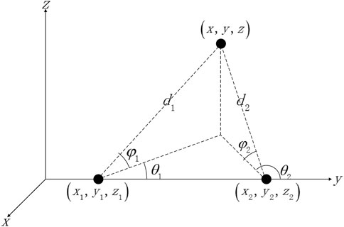
FIGURE 6. Diagram of the AOA method.

Let ${\theta }_i$ denote the horizontal angle at which the $i$ th known position point receives the signal to be monitored, and ${\phi }_i$ denote the pitch angle at which the $i$ th known position point receives the signal to be monitored. Therefore,

$\left\{\begin{array}{l}\Delta x=d_i\cos {\phi }_i\sin {\theta }_i\\ \Delta y=d_i\cos {\phi }_i\cos {\theta }_i\\ \Delta z=d_i\sin {\phi }_i\end{array}\right.(29)$

By solving the system of equations, the three-dimensional coordinates can be obtained. This is called the AOA method. The common way to solve the problem is to use geometric relations. The distance between two known position points is calculated and the sine law is used to determine $d_i$ and the three-dimensional coordinates.

The accuracy of the TDOA is proportional to the bandwidth of the received signal, and the accuracy of the AOA is not affected by it. In the case of a large signal bandwidth, TDOA measurements usually have higher acquisition accuracy than AOA measurements. Compared with the TDOA, the AOA localization performance is generally poor, so it is often combined with other algorithms. Sun Y. et al. proposed a new method called the constrained eigenspace (CES) to obtain AOA positioning solutions in modified polar representation (MPR) [114]. Yin J. et al. combined the AOA method and TDOA method and proposed a simple closed-form solution method, which only needed to use two observation stations [115]. Costa M. S. et al. combined the AOA method and RSS method and used the second-order cone programming (SOCP) relaxation technique to transform the non-convex estimator into a convex estimator. It has good performance and reduces computation [116]. Zuo P. et al. performed similar work based on the AOA method and RSS method [117].

4.5 Interference source tracking

From theory to simulation, interference source location technology often focuses on static interference sources. The purpose of interference source tracking is to track the interference source in motion. Based on the theory of interference source location, a Kalman filter algorithm is often involved. Biswas S. K. et al. combined the AOA and TDOA algorithms to compare the performance of various Kalman filtering algorithms for interference source tracking [118]. Biswas S. K. also proposed an interference source tracking algorithm based on the particle filter and compared it with the Kalman filter [119]. Qin N. et al. proposed a two-iteration interval extension method to determine the motion source using TDOA and FDOA information from multiple receivers [120]. Although interference tracking technology is only an extension of interference location technology, it still has room for development [121].

4.6 Brief summary

The use of measurements from multiple nodes for positioning dates back to the 1990s, partly because of satellite navigation technology. Among RSS methods, i.e., the TDOA method, FDOA method and AOA method, the TDOA method has the most mature technology, and the time information required by the TDOA method is also the easiest to obtain. In the field of satellite navigation, high-precision time alignment can be obtained through satellite signals, which provides support for positioning by the TDOA method. On the other hand, compared with the TDOA, the measurement accuracy of the FDOA has a greater impact on the positioning accuracy. This means that to ensure the accuracy of positioning, the measurement requirements for frequency measurement are more stringent than those for time measurement.

Interference tracking technology depends on Kalman filtering technology. The Kalman filter was developed in the 1960s. Using a Kalman filter, the estimation of the object motion trajectory is more accurate, and it is widely used in tracking moving objects. Compared with the classical algorithm of the 1940s, the Wiener filter and Kalman filter have been extended and achieved better performance, but the amount of computation is increased.

5 Prospect for interference monitoring technologies

5.1 Prospects for interference detection and recognition

Interference detection technology is divided into blanket interference detection technology and spoofing interference detection technology. The development of blanket interference detection technology is relatively complete. On the one hand, in many fields, such as communication and radar, there is similar RF interference, and the field of research is relatively rich. However, blanket interference forms are relatively simple, and the interference signal can be detected by energy detection in the time or frequency domain, which is easy to realize. The research on spoofing interference is different. Because of the characteristics of satellite navigation systems and their signals, spoofing interference in satellite navigation systems is specific. Some traditional methods have poor performance in detecting spoofing interference in the navigation field. In detection technology, there are several development directions. The first is the detection of weaker signals. Although the interference signals are often strong when subjected to human interference, to monitor the changes in the electromagnetic environment and achieve the function of early warning, it is necessary to have a certain monitoring ability for weak interference signals. The second is the interference of multiple interference sources, which is also common in actual scenarios. Therefore, the monitoring system must be able to detect multiple interference sources. Third, the monitoring system is faced with time-varying interference, which requires low computational complexity, fast computing speed, real-time performance and adaptive ability of interference detection and recognition equipment. Fourth, blanket interference and spoofing interference can exist at the same time, which requires the equipment to have the ability to recognize compound interference. It is common for both blanket interference and spoofing interference to exist in a real environment, while current theoretical research and simulation generally only consider one of them.

Interference recognition technology is mainly blind recognition. The frequency, amplitude and phase of the interference signal are not known before the received signal is processed. Therefore, feature parameters with a high separation degree should be extracted before interference signal identification. In the field of satellite navigation, there is little research on interference recognition technology. In the past, interference recognition technology was rarely analyzed alone. When an interference signal is detected, the relevant characteristics of the interference signal can be roughly obtained. With the increasing complexity of the electromagnetic environment and the increase in artificial interference means, it becomes important to distinguish the types of interference. With the development of machine learning, pattern recognition, deep learning and other computer fields, interference recognition technology has also been developed to a certain extent.

5.2 Prospects for interference source direction finding

The principle of amplitude methods is simple and easy to implement, but the precision is not good. Since the interference signals to the satellite signals are often attached to the carrier frequency, the wavelength of the interference signals is short, and the phase information is obvious. Therefore, phase methods, such as interferometer direction finding, have higher measurement accuracy than the previous amplitude method. Based on the theory of array signal processing and spatial spectrum estimation, the direction finding of multiple interference sources can be realized simultaneously. This makes the array antennas and spatial spectrum estimation more widely used in practice. Spatial spectrum estimation methods have high measurement accuracy, breaking the Rayleigh limit, and have the ability of super resolution direction finding. However, the algorithm has a high SNR requirement and a large amount of calculation, so it is difficult to carry out real-time processing. The main development of direction finding technology is the spatial spectrum estimation algorithm. First, spatial spectrum estimation algorithms usually require a large amount of computation, so GPU and other technologies can be used to improve the computational speed of spatial spectrum estimation algorithms. The second is compressed sensing, which can greatly reduce the number of antenna elements and sampled data. The third is to combine with cutting-edge fields such as machine learning.

5.3 Prospects for interference source location and tracking

The first development direction of interference source location technology is the joint algorithm, which can improve the accuracy of positioning and reduce the difficulty and cost of measurement, such as TDOA and FDOA common joint algorithms. Other forms of joint algorithms are generally feasible, such as the TDOA and AOA. The second is higher real-time performance. The interference source location algorithm also pursues higher computation speed. The third is the location of multiple interference sources. It is very common to face multiple interference sources in practice, and it is difficult to determine their locations.

Interference tracking technology is one of the possible development directions in the future. It is worth trying to improve the real-time performance of the interference location algorithm or improve the performance of a Kalman filter.

6 Conclusion

Interference monitoring technology is a part of the field of anti-interference. Different from interference suppression technology, which aims to weaken or eliminate the influence of interference signals, interference monitoring technology aims to monitor the electromagnetic environment, detect and identify interference signals, provide information for interference suppression, and make it possible to adopt more targeted algorithms. More importantly, interference monitoring technology can obtain the location and other information of the interference source before it sends out the interference to keep away from or destroy the interference source.

In the past, interference monitoring technology in the field of satellite navigation was always limited to detection and positioning. In fact, interference monitoring technology is a big concept; in practical applications, detection, recognition, direction finding, positioning, and tracking technology cross each other. With advances in fields such as machine learning, monitoring technology is getting smarter. With the development of GPUs and other technologies, the computing speed is increasing, and algorithms are more real-time. Interference monitoring technology is also more widely integrated with other fields, which makes it develop rapidly.

Author contributions

JQ wrote the manuscript of the paper, including the simulation and the pictures in the paper. ZL and JS provided the framework for the study, suggested changes to the paper and assisted in the revision of the paper. BJL, ZX, ZW, and BYL offered suggestions for the paper. All authors have read and agreed to the published version of the manuscript.

Funding

This research was funded by the National Natural Science Foundation of China (No. 62003354).

Acknowledgments

The authors would like to thank the editors and reviewers for their efforts to help the publication of this paper.

Conflict of interest

Author ZW is employed by Transcom (Shanghai) Technology Co., Ltd., Shanghai.

The remaining authors declare that the research was conducted in the absence of any commercial or financial relationships that could be construed as a potential conflict of interest.

Publisher’s note

All claims expressed in this article are solely those of the authors and do not necessarily represent those of their affiliated organizations, or those of the publisher, the editors and the reviewers. Any product that may be evaluated in this article, or claim that may be made by its manufacturer, is not guaranteed or endorsed by the publisher.

References

1. Yu K, Rizos C, Burrage D, Dempster A, Zhang K, Markgraf M. An overview of GNSS remote sensing. EURASIP J Adv Signal Process (2014) 134:134–14. doi:10.1186/1687-6180-2014-134

CrossRef Full Text | Google Scholar

2. Fejes I, Mihàly S. Interferometric approach in the NNSS data processing. Acta Astronautica (1985) 12:447–53. doi:10.1016/0094-5765(85)90051-7

CrossRef Full Text | Google Scholar

3. Bonnor N. A brief history of global navigation satellite systems. J Navigation (2012) 65:1–14. doi:10.1017/s0373463311000506

CrossRef Full Text | Google Scholar

4. Yalvac S. Investigating the historical development of accuracy and precision of Galileo by means of relative GNSS analysis technique. Earth Sci Inform (2021) 14:193–200. doi:10.1007/s12145-020-00560-8

CrossRef Full Text | Google Scholar

5. Kiliszek D, Kroszczyński K. Performance of the precise point positioning method along with the development of GPS, GLONASS and Galileo systems. Measurement (2020) 164:108009. doi:10.1016/j.measurement.2020.108009

CrossRef Full Text | Google Scholar

6. Xie J, Kang C. Engineering innovation and the development of the BDS-3 navigation constellation. Engineering (2021) 7:558–63. doi:10.1016/j.eng.2021.04.002

CrossRef Full Text | Google Scholar

7. Thombre S, Bhuiyan MZH, Söderholm S, Kirkko-Jaakkola M, Ruotsalainen L, Kuusniemi H. A software multi-GNSS receiver implementation for the Indian regional navigation satellite system. IETE J Res (2016) 62:246–56. doi:10.1080/03772063.2015.1093968

CrossRef Full Text | Google Scholar

8. Li X, Pan L, Yu W. Assessment and analysis of the four-satellite QZSS precise point positioning and the integrated data processing with GPS. IEEE Access (2021) 9:116376–94. doi:10.1109/access.2021.3106050

CrossRef Full Text | Google Scholar

9. Zidan J, Adegoke EI, Kampert E, Birrell SA, Ford CR, Higgins MD. GNSS vulnerabilities and existing solutions: A review of the literature. IEEE Access (2021) 9:153960–76. doi:10.1109/access.2020.2973759

CrossRef Full Text | Google Scholar

10.Threat Technology. Top 10 GPS spoofing events in history (2023). Available from: https://threat.technology/top-10-gps-spoofing-events-in-history/ (Accessed date August 4, 2022).

Google Scholar

11.Altereddimensions. FAA warns of unusual GPS interference this month from Top Secret China Lake weapons tests (2016). Available from: https://www.altereddimensions.net/2016/faa-warns-gps-interference-june-2016-top-secret-china-lake-weapons-tests (Accessed date August 5, 2022).

Google Scholar

12. Han Q, Zeng X, Li Z, Wang F. Recent development and prospect of interference monitoring for GNSS bands. Aerospace Electron warfare (2009) 17-19:29.

Google Scholar

13. Thombre S, Bhuiyan MZH, Eliardsson P, Gabrielsson B, Pattinson M, Dumville M, et al. GNSS threat monitoring and reporting: Past, present, and a proposed future. The J Navigation (2018) 71:513–29. doi:10.1017/s0373463317000911

CrossRef Full Text | Google Scholar

14. Li H, Liu A, Dou X, Liu J. Design and implementation of satellite navigation interference monitoring and positioning system. Radio Eng (2020) 50:219–26.

Google Scholar

15. Wu G. UAV-based interference source localization: A multimodal Q-learning approach. IEEE Access (2019) 7:137982–91. doi:10.1109/access.2019.2942330

CrossRef Full Text | Google Scholar

16. Wu G, Gu J. Remote interference source localization: A multi-UAV-based cooperative framework. Chin J Electron (2022) 31:442–55. doi:10.1049/cje.2021.00.310

CrossRef Full Text | Google Scholar

17. Sun X, Zhen W, Zhang F. GNSS interference source detection and location technology based on unmanned aerial vehicle. Gnss World of China (2021) 46:79–83.

Google Scholar

18. Ho KC, Sun M. Passive source localization using time differences of arrival and gain ratios of arrival. IEEE Trans Signal Process (2008) 56:464–77. doi:10.1109/tsp.2007.906728

CrossRef Full Text | Google Scholar

19. Lin X, He Y, Shi P. Location algorithm and error analysis for Earth object using TDOA,FDOA by dual-satellite and aided height information. Chin J Space Sci (2006) 4:277–82. doi:10.11728/cjss2006.04.277

CrossRef Full Text | Google Scholar

20. Wang W, Chen Z, Wang C. Single-satellite positioning algorithm based on direction-finding. In: 2017 Progress in electromagnetics research symposium - Spring (PIERS). St. Petersburg, Russia: IEEE (2017). doi:10.1109/PIERS.2017.8262179

CrossRef Full Text | Google Scholar

21. Simonsen K, Suycott M, Crumplar R, Wohlfiel J. LOCO GPSI: Preserve the GPS advantage for defense and security. IEEE Aerospace Electron Syst Mag (2004) 19:3–7. doi:10.1109/maes.2004.1374060

CrossRef Full Text | Google Scholar

22. Pelton JN. Radio-frequency geo-location and small satellite constellations. Handbook of Small Satellites (2020) 2020:811–23.

CrossRef Full Text | Google Scholar

23. Lu Z, Nie J, Chen F, Chen H, Ou G. Adaptive time taps of STAP under channel mismatch for GNSS antenna arrays. IEEE Trans Instrumentation Meas (2017) 66:2813–24. doi:10.1109/tim.2017.2728420

CrossRef Full Text | Google Scholar

24. Song J, Lu Z, Xiao Z, Li B, Sun G. Optimal order of time-domain adaptive filter for anti-jamming navigation receiver. Remote Sensing (2022) 14:48. doi:10.3390/rs14010048

CrossRef Full Text | Google Scholar

25. Lu Z, Song J, Huang L, Ren C, Xiao Z, Li B. Distortionless 1/2 overlap windowing in frequency domain anti-jamming of satellite navigation receivers. Remote Sensing (2022) 14:1801. doi:10.3390/rs14081801

CrossRef Full Text | Google Scholar

26. Xie X, Lu M, Zeng D. Research on GNSS generating spoofing jamming technology. In: IET International Radar Conference 2015. Hangzhou: IEEE (2015). doi:10.1049/cp.2015.0999

CrossRef Full Text | Google Scholar

27. Wang J, Su Z, Zhang Y. Study on optimal jamming signal of GPS system. Comput Meas Control (2016) 4:257–267.

Google Scholar

28. Gao Y, Li G. Three time spoofing algorithms for GNSS timing receivers and performance evaluation. GPS Solutions (2022) 26:87. doi:10.1007/s10291-022-01275-7

CrossRef Full Text | Google Scholar

29. Huang L, Lu Z, Xiao Z, Ren C, Song J, Li B. Suppression of jammer multipath in GNSS antenna array receiver. Remote sensing (2022) 14:350. doi:10.3390/rs14020350

CrossRef Full Text | Google Scholar

30. Mosavi M, Shafiee F. Narrowband interference suppression for GPS navigation using neural networks. GPS Solutions (2016) 20:341–51. doi:10.1007/s10291-015-0442-8

CrossRef Full Text | Google Scholar

31. Du R, Yue L, Yao S, Zhang D, Wang Y. Single-tone interference method based on frequency difference for GPS receivers. Prog Electromagnetics Res M (2019) 79:61–9. doi:10.2528/pierm18121602

CrossRef Full Text | Google Scholar

32. Merwe JRv. d., Garzia F, Rügamer A, Urquijo S, Franco DC, Felber W. Wide-band interference mitigation in GNSS receivers using sub-band automatic gain control. Sensors (2022) 22:679. doi:10.3390/s22020679

PubMed Abstract | CrossRef Full Text | Google Scholar

33. Li B, Qiao J, Lu Z, Yu X, Song J, Lin B, et al. Induction of attenuated Nocardia seriolae and their use as live vaccine trials against fish nocardiosis. Front Phys (2022) 131:10–20. doi:10.1016/j.fsi.2022.09.053

CrossRef Full Text | Google Scholar

34. Liu M, Han Y, Chen Y, Song H, Yang Z, Gong F. Modulation parameter estimation of LFM interference for direct sequence spread spectrum communication system in alpha-stable noise. IEEE Syst J (2021) 15:881–92. doi:10.1109/jsyst.2020.2991078

CrossRef Full Text | Google Scholar

35. Jian L, Yangbo H, Nie J, Wang F. Parameter selection analysis of matched spectrum interference. In: 2015 4th International Conference on Computer Science and Network Technology (ICCSNT). Harbin, China: IEEE (2015). doi:10.1109/ICCSNT.2015.7490977

CrossRef Full Text | Google Scholar

36. Ma P, Tang X, Lou S, Liu K, Ou G. Code tracking performance analysis of GNSS receivers with blanking model under periodic pulse interference. Radio Eng (2021) 30:184–95. doi:10.13164/re.2021.0184

CrossRef Full Text | Google Scholar

37. Borio D. GNSS acquisition in the presence of continuous wave interference. IEEE Trans Aerospace Electron Syst (2010) 46:47–60. doi:10.1109/taes.2010.5417147

CrossRef Full Text | Google Scholar

38. Psiaki ML, Humphreys TE. GNSS spoofing and detection. Proc IEEE (2016) 104:1258–70. doi:10.1109/jproc.2016.2526658

CrossRef Full Text | Google Scholar

39. Sheng Y, Li H, Zhou S, Zhang B. Research of GPS generated spoofing method. Foreign Electron Meas Technol (2018) 37:39–43.

Google Scholar

40. Pang C, Guo Z, Lv M, Zhang L, Zhai D, Zhang C. BDS against repeater deception jamming detection algorithm based on PNN. J Chin Inertial Technol (2021) 29:554–60.

Google Scholar

41. Kay S. Dimensionality reduction for signal detection. IEEE Signal Process. Lett (2022) 29:145–8. doi:10.1109/lsp.2021.3129453

CrossRef Full Text | Google Scholar

42. Nunes FD, Sousa FMG. Gnss blind interference detection based on fourth-order autocumulants. IEEE Trans Aerospace Electron Syst (2016) 52:2574–86. doi:10.1109/taes.2016.150499

CrossRef Full Text | Google Scholar

43. Huo S, Nie J, Wang F. Block-flow noise power estimation algorithm for pulsed interference detection of GNSS receivers. Electron Lett (2015) 51:1522–4. doi:10.1049/el.2015.1445

CrossRef Full Text | Google Scholar

44. Sun K, Jin T, Yang D. A new reassigned spectrogram method in interference detection for GNSS receivers. Sensors (2015) 15:22167–91. doi:10.3390/s150922167

PubMed Abstract | CrossRef Full Text | Google Scholar

45. Wang P, Cetin E, Dempster A, Wang Y, Wu S. GNSS interference detection using statistical analysis in the time-frequency domain. IEEE Trans Aerospace Electron Syst (2018) 54:416–28. doi:10.1109/taes.2017.2760658

CrossRef Full Text | Google Scholar

46. Lv Q, Qin H. A joint method based on time-frequency distribution to detect time-varying interferences for GNSS receivers with a single antenna. Sensors (2019) 19:1946. doi:10.3390/s19081946

PubMed Abstract | CrossRef Full Text | Google Scholar

47. Sun K, Yu B, Elhajj M, Ochieng WY, Zhang T, Yang J. A novel GNSS interference detection method based on smoothed pseudo-wigner-hough transform. Sensors (2021) 21:4306. doi:10.3390/s21134306

PubMed Abstract | CrossRef Full Text | Google Scholar

48. Motella B, Presti L. Methods of goodness of fit for GNSS interference detection. IEEE Trans Aerospace Electron Syst (2014) 50:1690–700. doi:10.1109/taes.2014.120368

CrossRef Full Text | Google Scholar

49. Wu Q, Zheng J, Dong Z, Su M, Liang H, Zhang P. Interference detection algorithm based on adaptive subspace tracking and RAIM for GNSS receiver. IET Radar, Sonar and Navigation (2018) 12:1028–37. doi:10.1049/iet-rsn.2018.5175

CrossRef Full Text | Google Scholar

50. Zhai S, Tang X, Huang T, Zhao X, Wu Y. A double threshold cooperative GNSS interference detection algorithm based on fuzzy logic. IEEE Access (2020) 8:177053–63. doi:10.1109/access.2020.3027612

CrossRef Full Text | Google Scholar

51. Silva FB, Cetin E, Martins WA. Radio frequency interference detection using nonnegative matrix factorization. IEEE Trans Aerospace Electron Syst (2022) 58:868–78. doi:10.1109/taes.2021.3111730

CrossRef Full Text | Google Scholar

52. Dehghanian V, Nielsen J, Lachapelle G. GNSS spoofing detection based on signal power measurements: Statistical analysis. Int J Navigation Observation (2012) 2012:1–8. doi:10.1155/2012/313527

CrossRef Full Text | Google Scholar

53. Vahid D, John N, Gerard L. GNSS spoofing detection based on receiver C/N_0 estimates. In: International Technical Meeting of Satellite Division of The Institute of Navigation. Nashville, Tennessee, US: IEEE (2012).

Google Scholar

54. Akos DM. Who's afraid of the spoofer? GPS/GNSS spoofing detection via automatic gain control (AGC). Navigation (2012) 59:281–90. doi:10.1002/navi.19

CrossRef Full Text | Google Scholar

55. Kang CH, Kim SY, Park CG. Adaptive complex-EKF-based DOA estimation for GPS spoofing detection. IET Signal Process. (2018) 12:174–81. doi:10.1049/iet-spr.2016.0646

CrossRef Full Text | Google Scholar

56. Magiera J. A multi-antenna scheme for early detection and mitigation of intermediate GNSS spoofing. Sensors (2019) 19:2411. doi:10.3390/s19102411

PubMed Abstract | CrossRef Full Text | Google Scholar

57. Lo SC, Enge PK. Authenticating aviation augmentation system broadcasts. In: IEEE/ION Position, Location and Navigation Symposium (PLANS 2010). Indian Wells, California, USA: IEEE (2010). doi:10.1109/PLANS.2010.5507223

CrossRef Full Text | Google Scholar

58. Li H, Hong L, Mingquan L. Global navigation satellite system spoofing-detection technique based on the Doppler ripple caused by vertical reciprocating motion. IET Radar, Sonar and Navigation (2019) 13:1655–64. doi:10.1049/iet-rsn.2019.0058

CrossRef Full Text | Google Scholar

59. Sun C, Cheong J, Dempster A, Zhao H, Feng W. GNSS spoofing detection by means of signal quality monitoring (SQM) metric combinations. IEEE Access (2018) 6:66428–41. doi:10.1109/access.2018.2875948

CrossRef Full Text | Google Scholar

60. Wang W, Li N, Wu R, Closas P. Detection of induced GNSS spoofing using S-Curve-Bias. Sensors (2019) 19:922. doi:10.3390/s19040922

PubMed Abstract | CrossRef Full Text | Google Scholar

61. Li J, Zhu X, Ouyang M, Li W, Chen Z, Dai Z. Research on multi-peak detection of small delay spoofing signal. IEEE Access (2020) 8:151777–87. doi:10.1109/access.2020.3016971

CrossRef Full Text | Google Scholar

62. Lewis SW, Chow CE, Geremia-Nievinski F, Akos DMM, Lo SC. GNSS interferometric reflectometry signature-based defense. Navigation (2020) 67:727–43. doi:10.1002/navi.393

CrossRef Full Text | Google Scholar

63. Humphreys TE. Detection strategy for cryptographic GNSS anti-spoofing. IEEE Trans Aerospace Electron Syst (2013) 49:1073–90. doi:10.1109/taes.2013.6494400

CrossRef Full Text | Google Scholar

64. Han S, Luo D, Meng W, Li C. Antispoofing RAIM for dual-recursion particle filter of GNSS calculation. IEEE Trans Aerospace Electron Syst (2016) 52:836–51. doi:10.1109/taes.2015.140297

CrossRef Full Text | Google Scholar

65. Khanafseh S, Roshan N, Langel S, Chan F-C, Joerger M, Pervan B. GPS spoofing detection using RAIM with INS coupling. In: 2014 IEEE/ION Position, Location and Navigation Symposium - PLANS 2014. Monterey, CA, USA: IEEE (2014). doi:10.1109/PLANS.2014.6851498

CrossRef Full Text | Google Scholar

66. Jeong S, Kim M, Lee J. CUSUM-Based GNSS spoofing detection method for users of GNSS augmentation system. Int J Aeronaut Space Sci (2020) 21:513–23. doi:10.1007/s42405-020-00272-9

CrossRef Full Text | Google Scholar

67. Shafiee E, Mosavi MR, Moazedi M. Detection of spoofing attack using machine learning based on multi-layer neural network in single-frequency GPS receivers. J Navigation (2018) 71:169–88. doi:10.1017/s0373463317000558

CrossRef Full Text | Google Scholar

68. Li J, Zhu X, Ouyang M, Li W, Chen Z, Fu Q. GNSS spoofing jamming detection based on generative adversarial network. IEEE Sensors J (2021) 21:22823–32. doi:10.1109/jsen.2021.3105404

CrossRef Full Text | Google Scholar

69. Zhang X, Liu C, Suen CY. Towards robust pattern recognition: A review. Proc IEEE (2020) 108:894–922. doi:10.1109/jproc.2020.2989782

CrossRef Full Text | Google Scholar

70. Mahadevkar SV, Khemani B, Patil S, Kotecha K, Vora DR, Abraham A, et al. A review on machine learning styles in computer vision—techniques and future directions. IEEE Access (2022) 10:107293–329. doi:10.1109/access.2022.3209825

CrossRef Full Text | Google Scholar

71. Kang C, Kim S, Park C. A GNSS interference identification using an adaptive cascading IIR notch filter. GPS Solutions (2014) 18:605–13. doi:10.1007/s10291-013-0358-0

CrossRef Full Text | Google Scholar

72. Ferre RM, de la Fuente A, Lohan ES. Jammer classification in GNSS bands via machine learning algorithms. Sensors (2019) 19:4841. doi:10.3390/s19224841

PubMed Abstract | CrossRef Full Text | Google Scholar

73. Chen X, He D, Yan X, Yu W, Truong TK. GNSS interference type recognition with fingerprint spectrum DNN method. IEEE Trans Aerospace Electron Syst (2022) 58:4745–60. doi:10.1109/taes.2022.3167985

CrossRef Full Text | Google Scholar

74. Lu Z, Nie J, Wan Y, Ou G. Optimal reference element for interference suppression in GNSS antenna arrays under channel mismatch. IET Radar, Sonar and Navigation (2017) 11:1161–9. doi:10.1049/iet-rsn.2016.0582

CrossRef Full Text | Google Scholar

75. Ni S, Ren B, Chen F, Lu Z, Wang J, Ma P, et al. GNSS spoofing suppression based on multi-satellite and multi-channel array processing. Front Phys (2022) 10. doi:10.3389/fphy.2022.905918

CrossRef Full Text | Google Scholar

76. Lu Z, Chen H, Chen F, Nie J, Ou G. Blind adaptive channel mismatch equalisation method for GNSS antenna arrays. IET Radar, Sonar and Navigation (2018) 12:383–9. doi:10.1049/iet-rsn.2017.0416

CrossRef Full Text | Google Scholar

77. Chan YT, Lee BH, Inkol R, Yuan Q. Direction finding with a four-element adcock-butler matrix antenna array. IEEE Trans Aerospace Electron Syst (2001) 37:1155–62. doi:10.1109/7.976956

CrossRef Full Text | Google Scholar

78. Sadler DJ. Accuracy of adcock watson-watt DF in the presence of channel errors. In: 2019 Sensor Signal Processing for Defence Conference (SSPD). Brighton, UK: IEEE (2019). doi:10.1109/SSPD.2019.8751643

CrossRef Full Text | Google Scholar

79. Wang J, Wang H, Zhao Y. Direction finding in frequency-modulated-based passive bistatic radar with a four-element adcock antenna array. IET Radar, Sonar and Navigation (2011) 5:807–13. doi:10.1049/iet-rsn.2010.0262

CrossRef Full Text | Google Scholar

80. Henault S, Antar YMM, Rajan S, Inkol R, Wang S. Effects of mutual coupling on the accuracy of adcock direction finding systems. IEEE Trans Aerospace Electron Syst (2012) 48:2990–3005. doi:10.1109/taes.2012.6324673

CrossRef Full Text | Google Scholar

81. Du W, Xie S. Mutual coupling analysis of Adcock Watson Watt direction finding system based on the receiving mutual impedance. In: ISAPE2012. Xian, China: IEEE (2012). doi:10.1109/ISAPE.2012.6408769

CrossRef Full Text | Google Scholar

82. Pan X, Dong J. Design and optimization of an ultrathin and broadband polarization-insensitive fractal FSS using the improved bacteria foraging optimization algorithm and curve fitting. Nanomaterials (2023) 13(1):191. doi:10.3390/nano13010191

PubMed Abstract | CrossRef Full Text | Google Scholar

83. Liu L, Yu T. An analysis method for solving ambiguity in direction finding with phase interferometers. Circuits, Systems, Signal Process. (2021) 40:1420–37. doi:10.1007/s00034-020-01536-1

CrossRef Full Text | Google Scholar

84. ŞengüL H, Gürel AE, Orduyilmaz A. Passive direction finding using correlative interferometer. In: 2021 29th Signal Processing and Communications Applications Conference (SIU). Istanbul, Turkey: IEEE (2021). doi:10.1109/SIU53274.2021.9477965

CrossRef Full Text | Google Scholar

85. Bai Y, Yang Z, Li R, Yang P, Ye J, Liu J. Research on single channel Doppler direction finding system. In: Proceedings of Eleventh International Conference on Digital Image Processing (ICDIP 2019). Guangdong, China: IEEE (2019). doi:10.1117/12.2540287

CrossRef Full Text | Google Scholar

86. Kummer W. Broad-band microwave electronically scanned direction finder. IEEE Trans Antennas Propagation (1983) 31:18–26. doi:10.1109/tap.1983.1143004

CrossRef Full Text | Google Scholar

87. Schmidt R. Multiple emitter location and signal parameter estimation. IEEE Trans Antennas Propagation (1986) 34:276–80. doi:10.1109/tap.1986.1143830

CrossRef Full Text | Google Scholar

88. Capon J. High-resolution frequency-wavenumber spectrum analysis. Proc IEEE (1969) 57:1408–18. doi:10.1109/proc.1969.7278

CrossRef Full Text | Google Scholar

89. Roy R, Paulraj A, Kailath T. ESPRIT-A subspace rotation approach to estimation of parameters of cisoids in noise. IEEE Trans Acoust Speech Signal Process (1986) 34:1340–2. doi:10.1109/tassp.1986.1164935

CrossRef Full Text | Google Scholar

90. Stoica P, Nehorai A. MUSIC, maximum likelihood, and cramer-rao bound. IEEE Trans Signal Process. (1989) 37:720–41. doi:10.1109/29.61541

CrossRef Full Text | Google Scholar

91. Cadzow JA. A high resolution direction-of-arrival algorithm for narrow-bandcoherent and incoherent sources. IEEE Trans Acoust Speech Signal Process (1988) 36:965–79. doi:10.1109/29.1618

CrossRef Full Text | Google Scholar

92. Clergeot H, Tressens S, Ouamri A. Performance of high resolution frequencies estimation methods compared to the Cramer-Rao bounds. IEEE Trans Acoust Speech, Signal Process (1989) 37:1703–20. doi:10.1109/29.46553

CrossRef Full Text | Google Scholar

93. Marcos S, Marsal A, Benidir M. The propagator method for source bearing estimation. Signal Process. (1995) 42:121–38. doi:10.1016/0165-1684(94)00122-g

CrossRef Full Text | Google Scholar

94. Porat B, Friedlander B. Direction finding algorithms based on high-order statistics. IEEE Trans Signal Process (1991) 39:2016–24. doi:10.1109/78.134434

CrossRef Full Text | Google Scholar

95. Yuan J, Zhang G, Zhang Y, Leung H. A gridless fourth-order cumulant-based DOA estimation method under unknown colored noise. IEEE Wireless Commun Lett (2022) 11:1037–41. doi:10.1109/lwc.2022.3153927

CrossRef Full Text | Google Scholar

96. Donoho DL. Compressed sensing. IEEE Trans Inf Theor (2006) 52:1289–306. doi:10.1109/tit.2006.871582

CrossRef Full Text | Google Scholar

97. Carlin M, Rocca P, Oliveri G, Viani F, Massa A. Directions-of-Arrival estimation through bayesian compressive sensing strategies. IEEE Trans Antennas Propagation (2013) 61:3828–38. doi:10.1109/tap.2013.2256093

CrossRef Full Text | Google Scholar

98. Ge S, Li K, Rum SNBM. Deep learning approach in DOA estimation: A systematic literature review. Mobile Inf Syst (2021) 2021:2021–14. doi:10.1155/2021/6392875

CrossRef Full Text | Google Scholar

99. Dempster AG, Cetin E. Interference localization for satellite navigation systems. Proc IEEE (2016) 104:1318–26. doi:10.1109/jproc.2016.2530814

CrossRef Full Text | Google Scholar

100. Wu R, Dong J, Wang M. Wearable polarization conversion metasurface MIMO antenna for biomedical applications in 5 GHz WBAN. Biosensors (2023) 13(1):73. doi:10.3390/bios13010073

PubMed Abstract | CrossRef Full Text | Google Scholar

101. Malaney RA. Nuisance parameters and location accuracy in log-normal fading models. IEEE Trans Wireless Commun (2007) 6:937–47. doi:10.1109/twc.2007.05247

CrossRef Full Text | Google Scholar

102. Thompson RJR, Cetin E, Dempster AG. Unknown source localization using RSS in open areas in the presence of ground reflections. In: IEEE/ION Position, Location and Navigation Symposium (PLANS 2012). Myrtle Beach, SC, USA: IEEE (2012). doi:10.1109/PLANS.2012.6236844

CrossRef Full Text | Google Scholar

103. Wang P, Morton YT. Efficient weighted centroid technique for crowdsourcing GNSS RFI localization using differential RSS. IEEE Trans Aerospace Electron Syst (2020) 56:2471–7. doi:10.1109/taes.2019.2917577

CrossRef Full Text | Google Scholar

104. Wang W, Zhang Y, Tian L. TOA-based NLOS error mitigation algorithm for 3D indoor localization. China Commun (2020) 17:63–72. doi:10.23919/jcc.2020.01.005

CrossRef Full Text | Google Scholar

105. Chan YT, Ho KC. A simple and efficient estimator for hyperbolic location. IEEE Trans Signal Process (1994) 42:1905–15. doi:10.1109/78.301830

CrossRef Full Text | Google Scholar

106. Foy WH. Position-location solutions by taylor-series estimation. IEEE Trans Aerospace Electron Syst (1976) 12:187–94. doi:10.1109/taes.1976.308294

CrossRef Full Text | Google Scholar

107. Zhang L, Zhang T, Shin H-S. An efficient constrained weighted least squares method with bias reduction for TDOA-based localization. IEEE Sensors J (2021) 21:10122–31. doi:10.1109/jsen.2021.3057448

CrossRef Full Text | Google Scholar

108. Díez-González J, Álvarez R, Verde P, Ferrero-Guillén R, Perez H. Analysis of reliable deployment of TDOA local positioning architectures. Neurocomputing (2022) 484:149–60. doi:10.1016/j.neucom.2021.12.074

CrossRef Full Text | Google Scholar

109. Uysal C, Filik T. A sparse TDOA estimation method for LPI source localization using distributed sensors. Wireless Personal Commun (2022) 123:2171–87. doi:10.1007/s11277-021-09233-1

CrossRef Full Text | Google Scholar

110. Liang Z, Yi W. Application of improved particle swarm optimization algorithm in TDOA. AIP Adv (2022) 12:025304–4. doi:10.1063/5.0082778

CrossRef Full Text | Google Scholar

111. Wang D, Zhang P, Yang Z, Wei F, Wang C. A novel estimator for TDOA and FDOA positioning of multiple disjoint sources in the presence of calibration emitters. IEEE Access (2020) 8:1613–43. doi:10.1109/access.2019.2959235

CrossRef Full Text | Google Scholar

112. Li G, Zhou M, Tang H, Chen H. A virtualization approach to correct systematic errors in measured TDOA and FDOA for low orbit dual-satellite positioning systems. Int J Antennas Propagation (2021) 2021:2021–11. doi:10.1155/2021/9631502

CrossRef Full Text | Google Scholar

113. Pine KC, Pine S, Cheney M. The geometry of far-field passive source localization with TDOA and FDOA. IEEE Trans Aerospace Electron Syst (2021) 57:3782–90. doi:10.1109/taes.2021.3087804

CrossRef Full Text | Google Scholar

114. Sun Y, Ho KC, Wan Q. Eigenspace solution for AOA localization in modified polar representation. IEEE Trans Signal Process (2020) 68:2256–71. doi:10.1109/tsp.2020.2981773

CrossRef Full Text | Google Scholar

115. Yin J, Wan Q, Yang S, Ho K. A simple and accurate TDOA-AOA localization method using two stations. IEEE Signal Process. Lett (2016) 23:144–8. doi:10.1109/lsp.2015.2505138

CrossRef Full Text | Google Scholar

116. Costa MS, Tomic S, Beko M. An SOCP estimator for hybrid RSS and AOA target localization in sensor networks. Sensors (2021) 21:1731. doi:10.3390/s21051731

PubMed Abstract | CrossRef Full Text | Google Scholar

117. Zuo P, Peng T, Wu H, You K, Jing H, Guo W, et al. Directional source localization based on RSS-AOA combined measurements. China Commun (2020) 17:181–93. doi:10.23919/jcc.2020.11.015

CrossRef Full Text | Google Scholar

118. Biswas SK, Cetin E. GNSS interference source tracking using kalman filters. In: 2020 IEEE/ION Position, Location and Navigation Symposium (PLANS). Portland, OR, USA: IEEE (2020). doi:10.1109/PLANS46316.2020.9109997

CrossRef Full Text | Google Scholar

119. Biswas SK, Cetin E. Particle filter based approach for GNSS interference source tracking: A feasibility study. In: 2020 XXXIIIrd General Assembly and Scientific Symposium of the International Union of Radio Science. Rome, Italy: IEEE (2020). doi:10.23919/URSIGASS49373.2020.9232443

CrossRef Full Text | Google Scholar

120. Qin N, Wang C, Shan C, Yang L. Interval analysis-based Bi-iterative algorithm for robust TDOA-FDOA moving source localisation. Int J Distributed Sensor Networks (2021) 17:155014772199177. doi:10.1177/1550147721991770

CrossRef Full Text | Google Scholar

121. Abdulkarim YI, Xiao M, Awl HN, Muhammadsharif FF, Lang T, Saeed SR, et al. Simulation and lithographic fabrication of a triple band terahertz metamaterial absorber coated on flexible polyethylene terephthalate substrate. Opt Mater Express (2022) 12:338–59. doi:10.1364/ome.447855

CrossRef Full Text | Google Scholar