Enhanced DQE and sub-pixel resolution by single-event processing in counting hybrid pixel electron detectors: A simulation study

Detective quantum efficiency (DQE) is a prominent figure of merit for imaging detectors, and its optimization is of fundamental importance for the efficient use of the experimental apparatus. In this work, I study the potential improvement offered by data processing on a single-event basis in a counting hybrid pixel electron detector (HPD). In particular, I introduce a simple and robust method of single-event processing based on the substitution of the original cluster of pixels with an isotropic Gaussian function. Key features are a better filtering of the noise power spectrum (NPS) and readily allowing for sub-pixel resolution. The performance of the proposed method is compared to other standard techniques such as centroiding and event normalization, in the simulated realistic scenario of 100 keV electrons impinging on a 450 μm-thick silicon sensor with a pixel size of 75 μm, yielding the best results. The DQE can potentially be enhanced over the entire spatial frequency range, increasing from 0.86 to nearly 1 at zero frequency and extending up to 1.40 times the physical Nyquist frequency of the system thanks to the sub-pixel resolution capability.

1 Introduction

Noise constitutes a fundamental limit to the detection efficiency of any radiation imaging system. Therefore, it is suitable to express the resolving power of a detector as the ratio between the signal and the noise (SNR). In the ideal case of a perfect imaging detector where each incoming particle is detected at its precise impinging position, the SNR is ultimately limited by the intrinsic variability given by the statistics of the incoming radiation. In the real world, any detector will introduce some additional noise for reasons mostly related to the physics involved in particle detection, to the mechanisms of signal generation, and to the interpretation and processing of the detected signal. As a metric of such worsening, it is customary to refer to the detective quantum efficiency (DQE) (see [1] and references therein for a historical overview), defined generically as follows:

$DQE=\frac{SN{R}_{\mathit{OUT}}^2}{SN{R}_{IN}^2}.(1)$

In the case of two-dimensional linear imaging systems, it is proper to extend the concept of DQE to the domain of spatial frequencies (μ, ν), leading to the following formulation [2]:

$DQE\left(\mu ,\nu \right)=\frac{MTF{\left(\mu ,\nu \right)}^2}{NNPS\left(\mu ,\nu \right)}\cdot \frac{1}{Q},(2)$

where MTF corresponds to the modulation transfer function, NNPS to the normalized noise power spectrum, obtained by dividing the NPS by the mean output signal, and Q to the incoming electron flux density, which corresponds to the SNR²_IN under the assumption of Poisson statistics. For simplicity and practicality reasons, the study of the DQE is often restricted to one single frequency coordinate (μ and ν being equivalent by symmetry) [3] in such a way that

$DQE\left(\nu \right)=DQE\left(0,\nu \right)=DQE\left(\mu ,0\right).(3)$

In the last decade, counting hybrid pixel detectors (HPD) have offered great advances in the field of X-ray diffraction experiments (XRD) [4, 5] and also shown great promises in other fields like non-destructive testing [6] and medical imaging [7, 8] because of key features like a large area, a large number of pixels, a fast frame rate, a wide dynamic range, no dark current, an excellent pixel point spread function, and no noise associated to the readout operation (provided a threshold level sufficiently higher than the electronic noise). Dose-independent DQE is also a noteworthy property [9]. For these reasons, these technologies have started being introduced to the field of electron microscopy, and many existing counting HPD like MEDIPIX2 [10], MEDIPIX3 [11], EIGER [12], EIGER2 [13], and IBEX [14] were investigated. For all electron detectors in general, and for dose-sensitive applications such as cryoEM [15] in particular, the quest for an optimization of the DQE performance is one of the driving forces of all the design phases, from the hardware to the image processing methods.

To this last category belongs the concept of single-event analysis. Electrons deposit energy in a semiconductor sensor along spatially randomized tracks, and depending on the electron energy, pixel size, and sensor thickness, the lateral spread can give rise to signals in (possibly several) neighboring pixels. Given the cluster of pixels pertaining to single events, the goal of the single-event analysis is to provide a better estimation of the real impinging position and/or reduce the signal variability (noise) among the pixel ensemble, improving the two fundamental ingredients of the DQE—the MTF and the NNPS, respectively. Several studies have already dealt with this topic. For example, [16–18] explored the benefits given by counting, centroiding, and event weighting in MAPS detectors; [19] applied several centroiding algorithms to a real case of cryoEM protein imaging again with MAPS detector; [20] further exploited the timing capabilities of a TIMEPIX3 detector applied to centroiding techniques in combination with a convolutional neural network, but the analysis was limited to the MTF. Centroiding is also the typical processing implemented in a commercial state-of-the-art direct detection detector (DDD) [21], and it typically allows for sub-pixel resolution, which is indeed attempted in [19, 20].

We can individuate some firm points:

i. The random nature of the electron track tends to diminish the correlation between energy deposition per pixel and real impinging positions [16, 17, 20]. This is expected, in particular, when the size of the electron tracks is greater than the (isotropic) contribution of the thermal diffusion and when the pixel size is not small enough to allow for a very fine spatial sampling of the deposited energy track. Typical counting detectors, therefore, do not suffer disadvantages with respect to detectors preserving the spectral information such as charge integrating detectors. 

ii. Centroiding techniques may improve the spatial localization of the event, thus improving the MTF, but the assignment of the full event to a selected pixel of the cluster increases the high-frequency component of the NNPS, degrading the DQE in that range [16, 17].

iii. In counting detectors operating in standard mode (no single-event analysis), the variability associated with the event multiplicity— the number of firing pixels per event—leads to a decrement of the DQE (0) for the reason presented in [10]:

$DQE\left(0\right)=\frac{\langle {m\rangle }^2}{\langle m^2\rangle },(4)$

where m is the probability distribution of the event multiplicity.

Normalizing to unity the events frees us from this relation and, leaving untouched the cluster shape, does not spoil the DQE at higher spatial frequencies [16].

iv. Methods involving sub-pixel resolution may lead to non-uniform filling of the sub-pixel matrix elements [20]. This effect is intrinsic to the method, and it is not ascribable to some non-ideal behavior of the detector. The important consequence is a possible worsening of the DQE (0) due to the different weights given to the noise of the sub-pixels in the final, flat-field corrected image.

In this work, I set up a numerical framework aimed to study and compare several single-event processing techniques in counting HPD. In addition to event centroiding and event normalization, used as reference, I devised a further, relatively simple and more effective processing method focused more on reducing the contribution of the NNPS rather than trying to improve the MTF only. In particular, each event is replaced by a normalized, isotropic two-dimensional Gaussian function centered on the event centroid and binned (integrated) over the surrounding pixels. The shape and parameters of such functions are retrieved from physical considerations. The possibility of sub-pixel resolution arises straightforwardly, and it is readily explored. The main advantages of this method are as follows: i) a potential enhancement of the DQE over all the frequency range and up to frequencies higher than the physical Nyquist frequency; ii) robustness, and iii) computationally fast. Practical considerations and limits of the method are also discussed. The range of usability extends to all dose-sensitive electron microscopy scenarios where optimized DQE is required, particularly in CryoEM applications. The scientific impact and popularity of this technique are indeed experiencing steady growth over the years, and single-event processing is already of customary use [22]. Despite being introduced in the context of counting HPD, the proposed method is, in principle, applicable to other counting devices, e.g., MAPS detectors, whose physics of signal generation and detection share many similarities with HPD.

As a case study for comparison, I chose to mimic a counting HPD consisting of a 450 μm-thick silicon sensor with a pixel size of 75 μm as a direct detection layer, bump-bonded to a counting read-out application-specific integrated circuit (ASIC). The impinging beam consists of electrons of energy 100 keV. For the sake of realism, I took the IBEX ASIC [23]as a reference. Incidentally, this simulated scenario corresponds to the experimental CryoEM setup used in [13].

2 Materials and methods

2.1 Simulation framework

The first step of the workflow was the computation of a statistically relevant database of electron tracks in the semiconductor sensor. A total of 40 million tracks impinging on the uniform (non-pixelated) side of the sensor were generated using FLUKA Monte Carlo code¹ [24, 25], storing, for each track, the three-dimensional spatial coordinates with an accuracy of 3 μm in all directions and the amount of energy deposited therein. The electron impinging position is uniformly distributed across the sensor surface, covering an area of 1024 × 1024 pixels.

A custom-developed software environment—an improved version of the one described and validated in [14]—processes each individual track to mimic the physics of the charge collection and signal formation at the pixelated electrode. The generated charge distribution of each track segment was thus propagated through the remaining sensor thickness to the pixels, and a Gaussian blurring was added to reproduce the effect the thermal diffusion, with a total width depending on an initial intrinsic contribution σ₀ and, under the assumption of the constant electric field, to a contribution depending on the total travel length:

$\sigma {\left(z\right)}^2={\sigma }_0^2+{\sigma }_{th,MAX}^2\frac{d-z}{d},(5)$

where d is the sensor thickness, z is the penetration depth measured from the impinging side, and σ_th,MAX is the maximum of the thermal diffusion contribution when z = 0. The charge collected by each pixel was converted into energy, and a counting threshold was applied—if the energy is higher, the pixel counts a 1; otherwise, it is 0. A random fluctuation, normally distributed and assumed uncorrelated among the pixels, was added to the signal, representing the electronic noise. The response of both the sensor and the read-out electronics has been assumed uniform in space. At this point, the statistical distribution of the event multiplicity can be extracted and, using Eq. 4, the corresponding DQE (0). The series of pixel clusters representing single events were then individually analyzed according to the methods described in Section 2.3 and then summed up to form two overall images, one used for the computation of the MTF and one for the computation of the NNPS. The one used for the MTF simulates the knife-edge experimental technique where half of the beam is blanked along a straight line slightly tilted (2°) with respect to the pixel matrix orientation. This is simply achieved by filtering events by the impinging position on the sensor. The one used for the NNPS consists, on the other hand, of a plain, uniformly filled image.

2.2 Simulation parameters

The simulated detector system consisted of a silicon sensor with a thickness of 450 μm and a pixel size p of 75 μm, read-out by a counting ASIC. The value of σ₀ was set to 2 μm rms and, at room temperature, the value of σ_th,MAX was estimated to be 7.5 μm rms. The value of the electronic noise contribution was set to 430 eV rms [26]. The threshold energy was set to 4 keV, close to the lowest practical limit available for the referenced chip. The choice of the threshold energy, in particular, in relation to the DQE (0), is analyzed in more in detail in Section 3.1.

2.3 Single-event processing and sub-pixel resolution

Different single-event processing techniques were investigated. As a ground reference, I refer to the standard counting case with no event processing as SC. As a relative term of comparison with previous works, I probed both the event normalization and the plain centroiding techniques, referred to as NORM and CoG, respectively. The NORM processing consists of scaling the count value of each pixel pertaining to a cluster by the total number of pixels forming the cluster such that every event counts as one. The CoG processing consists of computing the geometrical center of gravity of the pixel cluster and assigning the event to the pixel containing it.

The technique I propose aims to enhance the DQE by trying not to increase the MTF but rather to reduce the NNPS. To achieve this, processed events needs to have the following qualities: i) each of them counts as one (event normalization); ii) have a finite spatial extension (no collapse of the event cluster to a single pixel); and iii) have a smooth and isotropic shape. The last two requirements are of particular importance in order to efficiently reduce the high-frequency components of the NNPS in both spatial directions, which happens by introducing a correlation between neighboring pixels. The requirement of isotropicity arises from the consideration that single-event exhibits, in most cases, shapes with a certain degree of directionality, i.e., of anisotropicity, thus offering no natural attenuation to the high-frequency components of the noise along the direction “orthogonal” to the track line, where pixels have no correlation. Given these qualities, it is necessary to define the center and the specific shape of the processed event. As center, I chose the geometrical center of gravity, which, after all, retains some correlation with the real electron impinging position. As shape, I chose a Gaussian function, isotropic in the two spatial dimensions, which was found to nicely fit the probability distribution function of the position of the real impinging point relative to the centroid. This reflects, in a sort of average Bayesian inference, the uncertainty on the real impinging point given the event centroid. I refer to this method, the first of two, as G_SE, where the subscript stands for “semi-empirical,” being the knowledge of the impinging points made available using numerical simulations. In the second, “fully-empirical” method, referred to as G_E, the size of the Gaussian function was instead derived from the probability distribution of the distances of the firing pixels of the event cluster from the centroid. When the cluster consisted of more than one pixel, the contribution of each pixel was weighted with the inverse of the event multiplicity. It must be noted that this probability distribution is discrete in the two-dimensional space as a consequence of the basic fact that single events can assume only a discrete number of shapes and, therefore, the centroids can localize only at certain specific positions. In any case, the low-pass filtering effect is somehow tailored to the average size of the single-event. Examples of both probability distribution functions are provided in Section 3.2, associated with this specific case study. As a final step in either case, the continuous, Gaussian-shaped processed events must be binned into the pixel matrix. The binning was achieved by integrating the function over the area of the pixels in a neighboring area around the event center. Therefore, the expression of the count value c associated to the (i, j)-th pixel is as follows:

$c_{i,j}=\underset{x_i}{\overset{x_{i+1}}{\int }}\underset{y_j}{\overset{y_{j+1}}{\mathit{\int }}}\frac{1}{2\pi {\sigma }^2}\exp \left[-\frac{{\left(x-{\mathrm{c}\mathrm{o}\mathrm{g}}_x\right)}^2+{\left(y-{\mathrm{c}\mathrm{o}\mathrm{g}}_y\right)}^2}{2{\sigma }^2}\right]dxdy,(6)$

where cog is the geometrical center of gravity of the event and σ is the standard deviation computed according to the chosen method. Owing to the separability of the x and y components, the expression can be rewritten in terms of combination of error functions erf:

$c_{i,j}=\frac{1}{4}\left[\mathrm{e}\mathrm{r}\mathrm{f}\left(\frac{x_{i+1}-{\mathrm{c}\mathrm{o}\mathrm{g}}_x}{\sqrt{2}\sigma }\right)-\mathrm{e}\mathrm{r}\mathrm{f}\left(\frac{x_i-{\mathrm{c}\mathrm{o}\mathrm{g}}_x}{\sqrt{2}\sigma }\right)\right]\left[\mathrm{e}\mathrm{r}\mathrm{f}\left(\frac{y_{j+1}-{\mathrm{c}\mathrm{o}\mathrm{g}}_y}{\sqrt{2}\sigma }\right)-\mathrm{e}\mathrm{r}\mathrm{f}\left(\frac{y_j-{\mathrm{c}\mathrm{o}\mathrm{g}}_x}{\sqrt{2}\sigma }\right)\right],(7)$

which is easy to compute numerically.

The CoG, G_SE, and G_E can be used to improve the spatial resolution of the system below the geometrical limit set by the pixel size, thus achieving sub-pixel resolution. Each original pixel was subdivided into a matrix of n × n sub-pixels of equal size, and the event centroid was assigned to the sub-pixel containing it. I explored oversampling factors n up to 3 (in the following, the oversampling factor associated with a specific processing method is indicated as a subscript), as for higher values, no further improvement was observed in this specific case study. An intrinsic problem of the oversampling was that event centroids do not necessarily fill the sub-pixel matrix equally as a consequence of their discrete distribution on the two-dimensional space. According to the relative probabilities of occurrence of the different cluster shapes—dictated by the physical case—the distribution of the centroids can be skewed, e.g., toward the central sub-pixel, to the lateral ones along the border between neighboring pixels or the ones at the corners of the original pixel. Given the symmetry of the problem along the x and y directions, the sub-pixel response matrix also exhibits a diagonal symmetry. An additional source of non-uniformity lies in the arbitrariness in the assignment of the sub-pixel containing the centroid when the centroid is located on the boundary among neighboring sub-pixels and a rounding rule has to be set. The overall, undesired effect is then to generate a pattern reflecting the structure of the sub-pixel response in the final image, obtained by summing all processed events. The effect is stronger for the CoG method, which has the highest degree of event “localization,” while it is milder for both G_E and G_SE methods in virtue of their spatial blurring, which potentially spans over several neighboring pixels. The mandatory restoration of the uniformity in the final image can be achieved by dividing the value of each new (sub-)pixel by the value of the corresponding position in the sub-pixel response map as a classic flat-field correction. The sub-pixel response map can be computed as the average signal value at each specific sub-pixel location under the condition of uniform illumination, followed by normalization in order to have the mean value of the sub-pixel response map equal to 1 (needed to preserve the magnitude of the detected signal). In this idealistic scenario, the flat-field correction factors are perfectly defined and not subject to statistical and/or systematic errors. There is, however, a side effect. The multiplication of the value of each pixel by scalar weight is in a different way than the associated noise. In particular, the noise of low-counting pixels is amplified more than the noise of high-counting pixels is reduced, leading to an overall reduction of the SNR (0)_out and, therefore, of the DQE (0) in reason of the harmonic mean of the sub-pixel response map. Proof of this statement is given in Appendix.

3 Results and discussion

3.1 Multiplicity distribution and DQE (0) vs. threshold energy

In counting HPD, the threshold energy is a setting that can critically influence the performance. In order to find a reasonable value for this study, I investigated its influence on the DQE (0) by studying the multiplicity distributions and using Eq. 4; Figure 1 shows the cumulative probability distributions of the multiplicity as a function of the threshold energy. Multiplicities higher than 4 have negligible occurrence and were omitted. The average multiplicity value as a function of the threshold energy is also shown. The resulting DQE (0) is plotted in Figure 2. The half-beam energy threshold value (50 keV) clearly separates two different behavior regimes. Below this value, the DQE (0) is almost constant within the range of 0.81–0.86. This indicates that the ratio between ⟨m⟩² and ⟨m²⟩ remains basically stable, although both quantities increase for decreasing thresholds. Only below ∼4 keV, the DQE (0) raises a bit, but the improvement is limited to a few percent. On the other hand, for increasing the energy threshold above half-beam energy, the DQE (0) decreases progressively. In this regime, m = {0, 1} (in no way an electron can deposit more than half of its energy in more than one pixel), and Eq. 4 simplifies to DQE (0) = ⟨m⟩, whose decreasing behavior is obvious. For the purpose of the DQE (0), the threshold energy should, thus, be set as low as possible. At the chosen, realistic threshold of 4 keV, ⟨m⟩ = 1.99, ⟨m²⟩ = 4.74 and, therefore, DQE (0) = 0.86.

FIGURE 1

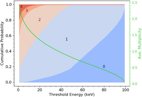
FIGURE 1. On the left-hand side axis, the event multiplicity cumulative probability distributions as a function of the threshold energy. Multiplicities higher than 4 have negligible occurrence and are not shown. On the right-hand side axis (green), the average event multiplicity.

FIGURE 2

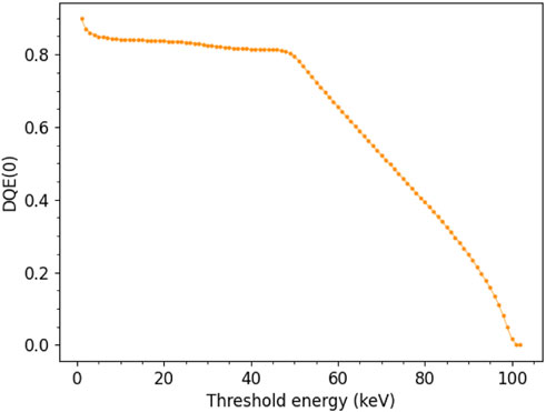
FIGURE 2. DQE (0) obtained from the event multiplicity distributions using Eq. 4.

3.2 Spatial distribution of impinging points and firing pixels with respect to the centroid

Figure 3 shows the two-dimensional statistical distribution of the distance of the real impinging point from the event centroid. For visibility reasons, a brighter color in the scatter plot means higher a value of probability density. The impinging points look genuinely randomly distributed around the centroid, and the shape is well-described by a bivariate normal distribution, whose fitting yields a value for the standard deviation of 0.24 pixel rms in both directions. This number was then used in the G_SE method. The x and y marginal distributions of the simulated data and of the two-dimensional Gaussian fitting are also shown in the top and right-hand side panels. Figure 4 shows the two-dimensional statistical distribution of the distance of the firing pixels from the event centroid. Also, in this case, to guide the eye, brighter color and bigger symbol size in the scatter plot mean a higher value of probability density. The discrete nature of the distribution—consequence of the finite number of shapes clusters can assume (as mentioned in Section 2.3)—appears evident. The standard deviation of the bivariate normal distribution arbitrarily used to fit this dataset amounts to 0.35 pixel rms, the value that is used in the G_E method.

FIGURE 3

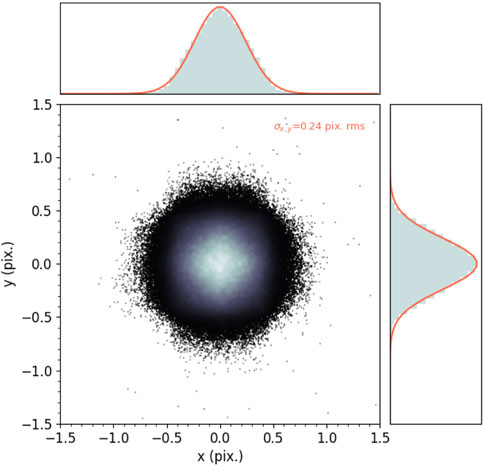
FIGURE 3. Statistical distribution of the distance of the real impinging point from the event centroid. A brighter color means a higher probability density value. On top and on the right-hand side, the x and y marginal distributions of the simulated data and of the two-dimensional Gaussian fitting.

FIGURE 4

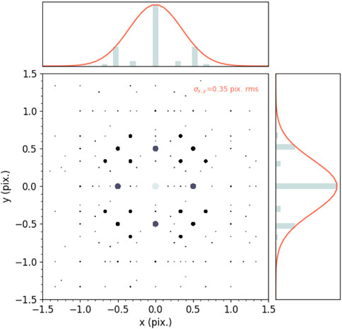
FIGURE 4. Statistical distribution of the distance of the firing pixels from the event centroid. Brighter color and bigger symbol dimension mean higher probability density values. On top and on the right-hand side, the x and y marginal distributions of the simulated data and of the two-dimensional Gaussian fitting.

3.3 Imaging metrics vs. processing method

With the help of Figure 5 we can visualize, for illustration purposes, the effect of the several probed processing methods and oversampling factors on an exemplary case of a single event. The position of the centroid and of the real impinging point is also shown as a reference. The isotropic blurring given by methods G_SE and G_E is clearly recognizable.

FIGURE 5

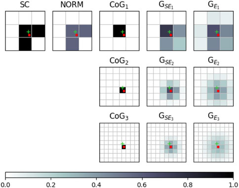
FIGURE 5. Example of single event processing for each of the probed processing methods. Symbol (+) represents the real impinging point, and (o) represents the computed center of gravity.

Figure 6 shows the sub-pixel response maps resulting from the processing methods with an oversampling factor greater than 1. Sub-pixel intensities are indicated both with color code and with the corresponding numerical value. As expected, the highest variation among the sub-pixels is observed for the CoG case. In particular, with an oversampling factor of 3, one can observe the extreme degeneration of some elements of the matrix to zero. This result leads to an undefined behavior when applying the sub-pixel correction to the overall image due to division by zero, and therefore, the study of the CoG₃ was discontinued. Higher oversampling factors (not shown here) for CoG were found to lead to the same situation. On the other hand, G_SE and G_E methods yielded much more uniform results by virtue of their low-pass filtering effect, especially for oversampling factor 2. For oversampling factor 3, some non-uniformity is left, in particular, for G_SE, due to its shorter spatial correlation range.

FIGURE 6

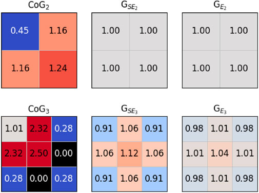
FIGURE 6. Sub-pixel response maps for each of the probed processing methods with an oversampling factor higher than 1.

Figure 7 shows the MTF for the different processing methods. The frequency range is expressed both in absolute value and as fraction of the physical Nyquist limit, which corresponds to ν_Ny=(2p)⁻¹ = 6.67 mm^-1. The sinc function corresponding to the MTF of the ideal pixel is also shown for comparison. All processing methods, except the G_E, slightly improve the MTF with respect to the SC case, with the biggest improvement by far being given by the CoG₂. For increasing oversampling factor also, the MTF of G_E and G_SE increases, but the enhancement is more pronounced stepping from oversampling factor 1 to 2 rather than from 2 to 3.

FIGURE 7

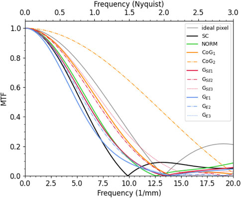
FIGURE 7. MTF for the different probed processing methods. The frequency range is expressed both in absolute values and as a fraction of the physical Nyquist limit.

Figure 8 shows the NNPS as a function of the spatial frequency for the different processing methods. For normalization purposes, the NNPS was multiplied by the scalar Q (see Eq. 2). In this way, the behavior of the ideal pixel matrix with Poissonian uncorrelated noise leads to a flat line of value 1, also shown as a term of comparison. At zero frequency, all methods involving event normalization and CoG₁ exhibit a value close to the theoretical limit and sensibly lower than the unprocessed SC method. A remaining tiny noise excess with respect to the ideal case is due to the effect of the non-uniformity of the sub-pixel response map. For the CoG₂ method, which suffers the highest non-uniformity in the sub-pixel response map, this effect is, on the contrary, macroscopic. At higher spatial frequencies, a clear distinction between CoG and all the other methods can be observed. In the CoG cases, the collapse of the events to individual pixels leads to completely uncorrelated pixels, and therefore, the corresponding NNPS remains flat over all the frequency ranges. In all the other cases, the corresponding NNPS exhibits a decreasing behavior for increasing spatial frequencies. The low-pass filtering effect, already naturally present in the SC case, is enhanced by the G_E methods over all the ranges and for all oversampling factors. A milder roll-off is instead noticeable for the G_SE and NORM methods, which intersect the curve of the SC method at roughly ν_Ny/2. For oversampling factors greater than 1, the NNPS of both G_SE and G_E methods keeps decreasing monotonically up to the corresponding oversampled Nyquist frequencies.

FIGURE 8

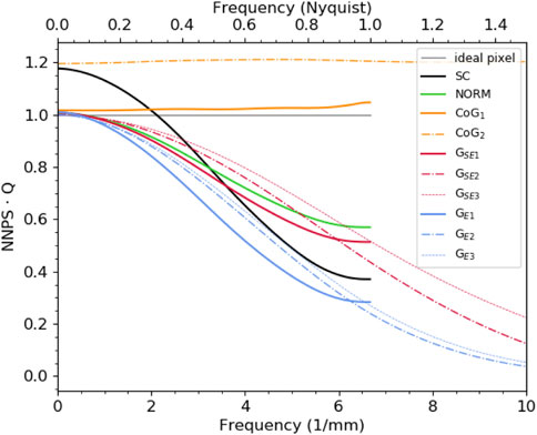
FIGURE 8. NNPS for the different probed processing methods. For normalization purposes, the NNPS was multiplied by the scalar Q. The frequency range is expressed both in absolute values and as a fraction of the physical Nyquist limit.

Finally, Figure 9 shows the resulting DQE. The sinc² function corresponding to the DQE of the ideal pixel is also shown for comparison. Incidentally, I would like to point out that both the DQE and the MTF of the SC method are in excellent agreement with the experimental data shown in [14].² At zero frequency, all methods involving normalization of the events and CoG₁ have a higher DQE value with respect to the SC method and are close to the theoretical limit of 1. CoG₂ has, on the other hand, the worst performance. At higher spatial frequencies methods, SC and, above ν_Ny/2, NORM and G_SE1 behave similarly and close to the curve of the ideal pixel. A tiny improvement is noticeable for G_E1 in virtue of its longer spatial correlation range that makes the effect of the isotropicity more efficient (both the MTF and the NNPS decrease, but the net effect is in favor of the DQE). In this high-frequency range, the CoG₁ has the worst performance. It is, however, for oversampling factors higher than 1 that the G_SE and G_E methods reveal their true superiority. In order to quantify the performance, one can look at the “critical” frequency value ν_C such that DQE (ν_C) is equal to DQE (ν_Ny) of the ideal pixel case, which amounts to 0.405 (to guide the eye, it is drawn in Figure 9 as a horizontal line). While all methods with oversampling factor 1 (excluded CoG₁) have a similar critical frequency at around 0.94 ν_Ny—which means an effective pixel size p_E=(2ν_Ny)⁻¹ = 1.06 p—G_SE2,3 and G_E2,3 methods have a critical frequency in the range 1.32 ν_Ny–1.40 ν_Ny, meaning an effective pixel size of 0.71 p–0.76 p. Also, CoG₂ has a critical frequency of 1.37 ν_Ny, but it pays the price of a poorer DQE (0). All these figures of merit are summarized in Table 1.

FIGURE 9

FIGURE 9. DQE for the different probed processing methods. The frequency range is expressed both in absolute values and as a fraction of the physical Nyquist limit of the detector.

TABLE 1

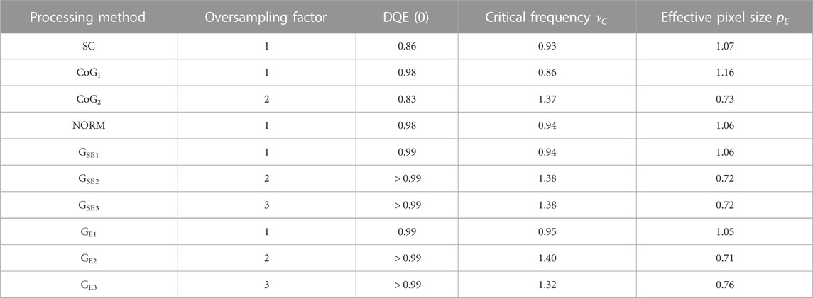
TABLE 1. Summary of the probed filters. Lengths are expressed in the physical pixel unit, and frequencies are expressed in the physical Nyquist unit.

3.4 Generalization and limits of usability

From the obtained results, we can infer some general properties:

a. CoG methods are very sensitive to the uneven (and discretized) geometrical distribution of the centroids. This clearly appears in the non-uniformity of the sub-pixel response maps, particularly for increasing oversampling factors. The spatial distribution of the centroids is also strongly related to the particular physical case under analysis (electron beam energy, sensor material, and geometry) and, therefore, so does the DQE.

b. The NORM method works well, but it is not scalable to oversampling factors higher than 1 and, therefore, cannot be exploited to achieve sub-pixel resolution.

c. The proposed family of methods G not only guarantees robustness against non-uniform centroid distributions, due to the spatial blurring, but is also readily scalable to any arbitrary oversampling factor. A general pre-condition for reasonable use of pixel oversampling is to have a physical pixel size of roughly the same magnitude or slightly smaller than the average lateral spread of the electron track. For bigger pixel sizes, indeed, the number of events with multiplicity higher than 1 decreases sensibly, preventing, in many cases, the computation of the event centroid with sub-pixel information; for smaller pixel sizes, on the other hand, electron tracks are naturally oversampled by the detector, and a further division into sub-pixels give minimal to no additional useful information. At intermediate cases, it is reasonable to assume that the optimal oversampling factor is in the range of 2–3, like the example examined in this work.

d. The fact that I observed almost no difference between the DQE of G_SE and G_E methods questions the importance of the spatial width (σ) of the processed events. In this work, I derived this parameter from physical considerations, but nothing prevents a more pragmatic approach where such width is optimized empirically.

3.5 Practical considerations

In a realistic scenario, the use of an oversampling factor higher than 1 requires the preliminary step of computing the sub-pixel response map necessary for the correction of the final overall image. This task can be accomplished by applying the single-event analysis on images (or sub-regions of images) recorded under uniform illumination and by averaging the corresponding sub-pixel position of the entire macro-pixel matrix and normalizing the obtained values by their mean. Additional statistical and/or systematic errors in the computation of the flat-field correction factors, typical of any real-world detection system, would also concur with the worsening of the imaging performances, although, in typical circumstances, it should not be severe. As an example, a random error with zero average and 1% (5%) standard deviation would lead to a decrease of the DQE (0) of only ∼0.005% (∼0.12%), according to Eq. 20 in Appendix.

4 Conclusion

I devised a simple and robust single-event processing method for counting HPD based on replacing the original event with an isotropic two-dimensional Gaussian function. I investigated the potential improvements in terms of DQE with respect to the unprocessed case and other well-known processing techniques, namely, event normalization and centroiding. In my method, the Gaussian function representing the event is centered at the event centroid and has a unitary integral. The spatial width was retrieved in two ways. In the first, semi-empirical way (it requires preliminary Monte Carlo simulations) G_SE, from the statistical distribution of the real impact position of the electrons with respect to the event centroid; in the second, fully empirical way G_E, from the statistical distribution of the firing pixels with respect to the event centroid. The rationale of my method is to enhance the DQE not by improving the MTF but rather by reducing the NPS, by virtue of its spatial low-pass filtering effect, which reflects the intrinsic natural uncertainty in the localization of the detected event. The method, readily scalable to oversampling factors higher than 1 and due to the higher uniformity of the sub-pixel response map, can efficiently achieve sub-pixel resolution capabilities. With possible uses in all dose-sensitive applications where optimized DQE is required, CryoEM, above all, the method is in principle applicable to other counting devices like MAPS detectors.

I numerically investigated the realistic case study of 100 keV electrons impinging on a 450 μm-thick silicon sensor with a pixel size of 75 μm at the threshold energy of 40 keV. At zero spatial frequency, the proposed method’s G_SE and G_E enhance the DQE as much as the other methods involving event normalization (NORM, CoG₁) from 0.86 of the SC method to nearly the theoretical limit of 1. At higher spatial frequencies and for oversampling factors higher than 1, on the other hand, they demonstrate the highest DQE among all the probed methods and allow for an extension of the effective Nyquist frequency up to 1.40 times the physical one, meaning a corresponding pixel size 0.71 times the physical one. This is without significant differences between G_SE and G_E and between oversampling factors 2 and 3.

While the behavior of the proposed technique depends on the particular physical case under analysis in general, I expect a good performance for all those cases where the pixel size is roughly comparable to the average lateral spread of the electron track. The optimal oversampling factor is also not expected not to exceed 3, although 2 could already be satisfying like in the analyzed case. As an outlook, further studies should be devoted to clarifying the dependence, in this case almost negligible, of the spatial width parameter of the G methods on the DQE.

Data availability statement

The raw data supporting the conclusion of this article will be made available by the author, without undue reservation.

Author contributions

The author confirms being the sole contributor of this work and has approved it for publication.

Acknowledgments

The author would like to deeply thank Valeria Radicci for the support with the Monte Carlo simulations and Michael Rissi and Christian Disch for the fruitful discussions.

Conflict of interest

Author PZ is employed by DECTRIS Ltd.

Publisher’s note

All claims expressed in this article are solely those of the authors and do not necessarily represent those of their affiliated organizations, or those of the publisher, the editors, and the reviewers. Any product that may be evaluated in this article, or claim that may be made by its manufacturer, is not guaranteed or endorsed by the publisher.

Footnotes

¹v. 4–2.1. The physics was set to multiple Coulomb scattering with cutoff energy of 1 keV for electrons and 100 eV for photons. Fluorescence was enabled, and no biasing was used.

²I refers to the measurements taken at the threshold energy of 5 keV.

References

1. Ji X, Feng M, Zhang R, Chen G-H, Li K. An experimental method to directly measure DQE(k) at k  =  0 for 2D x-ray imaging systems. Phys Med Biol (2019) 64(7):075013. doi:10.1088/1361-6560/ab10a2

PubMed Abstract | CrossRef Full Text | Google Scholar

2. Bath M. Evaluating imaging systems: Practical applications. Radiat Prot Dosimetry (2010) 139:26–36. doi:10.1093/rpd/ncq007

PubMed Abstract | CrossRef Full Text | Google Scholar

3. Williams MB, Mangiafico PA, Simoni PU. Noise power spectra of images from digital mammography detectors. Med Phys (1999) 26:1279–93. doi:10.1118/1.598623

PubMed Abstract | CrossRef Full Text | Google Scholar

4. Broennimann C, Eikenberry EF, Henrich B, Horisberger R, Huelsen G, Pohl E, et al. The PILATUS 1M detector. J Synchrotron Radiat (2006) 13:120–30. doi:10.1107/s0909049505038665

PubMed Abstract | CrossRef Full Text | Google Scholar

5. Casanas A, Warshamanage R, Finke AD, Panepucci E, Olieric V, Noll A, et al. EIGER detector: Application in macromolecular crystallography. Acta Crystallogr D (2016) 72:1036–48. doi:10.1107/s2059798316012304

PubMed Abstract | CrossRef Full Text | Google Scholar

6. Hanke R, Fuchs T, Uhlmann N. X-ray based methods for non-destructive testing and material characterization. Nucl Instrum Methods Phys Res A (2008) 591:14–8. doi:10.1016/j.nima.2008.03.016

CrossRef Full Text | Google Scholar

7. Koenig T, Schulze J, Zuber M, Rink K, Butzer J, Hamann E, et al. Imaging properties of small-pixel spectroscopic X-ray detectors based on cadmium telluride sensors. Phys Med Biol (2012) 57:6743–59. doi:10.1088/0031-9155/57/21/6743

PubMed Abstract | CrossRef Full Text | Google Scholar

8. Taguchi K, Iwanczyik JS. Vision 20/20: Single photon counting X-ray detectors in medical imaging. Med Phys (2013) 40:100901. doi:10.1118/1.4820371

PubMed Abstract | CrossRef Full Text | Google Scholar

9. Gkoumas S, Thuering T, Taboada AG, Jensen A, Rissi M, Broennimann C, Zambon P. Dose-independent near-ideal DQE of a 75 μm pixel GaAs photon counting spectral detector for breast imaging. In: Proc. SPIE 10948, Medical Imaging 2019: Physics of Medical Imaging; 1 March 2019; California, United States (2019).

CrossRef Full Text | Google Scholar

10. McMullan G, Cattermole D, Chen S, Henderson R, Llopart X, Summerfield C, et al. Electron imaging with Medipix2 hybrid pixel detector. Ultramicroscopy (2007) 107:401–13. doi:10.1016/j.ultramic.2006.10.005

PubMed Abstract | CrossRef Full Text | Google Scholar

11. Mir JA, Clough R, MacInnes R, Gough C, Plackett R, Shipsey I, et al. Characterisation of the Medipix3 detector for 60 and 80 keV electrons. Ultramicroscopy (2017) 182:44–53. doi:10.1016/j.ultramic.2017.06.010

PubMed Abstract | CrossRef Full Text | Google Scholar

12. Tinti G, Marchetto H, Vaz CAF, Kleibert A, Andrä M, Barten R, et al. The EIGER detector for low-energy electron microscopy and photoemission electron microscopy. J Synchrotron Rad (2017) 24:963–74. doi:10.1107/s1600577517009109

PubMed Abstract | CrossRef Full Text | Google Scholar

13. Naydenova K, McMullan G, Peet MJ, Lee Y, Edwards PC, Chen S, et al. CryoEM at 100 keV: A demonstration and prospects. IUCrJ (2019) 6:1086–98. doi:10.1107/s2052252519012612

PubMed Abstract | CrossRef Full Text | Google Scholar

14. Fernandez-Perez S, Boccone V, Broennimann C, Disch C, Piazza L, Radicci V, et al. Characterization of a hybrid pixel counting detector using a silicon sensor and the IBEX readout ASIC for electron detection. J Instrum (2021) 16:P10034. doi:10.1088/1748-0221/16/10/p10034

CrossRef Full Text | Google Scholar

15. Peet MJ, Henderson R, Russo CJ. The energy dependence of contrast and damage in electron cryomicroscopy of biological molecules. Ultramicroscopy (2019) 203:125–31. doi:10.1016/j.ultramic.2019.02.007

PubMed Abstract | CrossRef Full Text | Google Scholar

16. McMullan G, Clark AT, Turchetta R, Faruqi AR. Enhanced imaging in low dose electron microscopy using electron counting. Ultramicroscopy (2009) 109:1411–6. doi:10.1016/j.ultramic.2009.07.004

PubMed Abstract | CrossRef Full Text | Google Scholar

17. McMullan G, Turchetta R, Faruqi AR. Single event imaging for electron microscopy using MAPS detectors. J Instrum (2011) 6:C04001. doi:10.1088/1748-0221/6/04/c04001

CrossRef Full Text | Google Scholar

18. McMullan G, Faruqi AR, Clare D, Henderson R. Comparison of optimal performance at 300keV of three direct electron detectors for use in low dose electron microscopy. Ultramicroscopy (2014) 147:156–63. doi:10.1016/j.ultramic.2014.08.002

PubMed Abstract | CrossRef Full Text | Google Scholar

19. Zhu D, Shi H, Wu C, Zhang X. An electron counting algorithm improves imaging of proteins with low-acceleration-voltage cryoelectron microscope. Commun Biol (2022) 5:321. doi:10.1038/s42003-022-03284-1

PubMed Abstract | CrossRef Full Text | Google Scholar

20. van Schayck JP, van Genderen E, Maddox E, Roussel L, Boulanger H, Fröjdh E, et al. Sub-pixel electron detection using a convolutional neural network. Ultramicroscopy (2020) 218:113091. doi:10.1016/j.ultramic.2020.113091

PubMed Abstract | CrossRef Full Text | Google Scholar

21. Guo H, Franken E, Deng Y, Benlekbir S, Singla Lezcano G, Janssen B, et al. Electron-event representation data enable efficient cryoEM file storage with full preservation of spatial and temporal resolution. IUCrJ (2020) 7:860–9. doi:10.1107/s205225252000929x

PubMed Abstract | CrossRef Full Text | Google Scholar

22. Renaud J-P, Chari A, Ciferri C, Liu W-t., Rémigy H-W, Stark H, et al. Cryo-EM in drug discovery: Achievements, limitations and prospects. Nat Rev Drug Discov (2018) 17:471–92. doi:10.1038/nrd.2018.77

PubMed Abstract | CrossRef Full Text | Google Scholar

23. Bochenek M, Bottinelli S, Broennimann C, Livi P, Loeliger T, Radicci V, et al. Ibex: Versatile readout ASIC with spectral imaging capability and high count rate capability. IEEE Trans Nucl Sci (2018) 65:1285–91. doi:10.1109/tns.2018.2832464

CrossRef Full Text | Google Scholar

24. Böhlen T, Cerutti F, Chin M, Fassò A, Ferrari A, Ortega P, et al. The FLUKA code: Developments and challenges for high energy and medical applications. Nucl Data Sheets (2014) 120:211–4. doi:10.1016/j.nds.2014.07.049

CrossRef Full Text | Google Scholar

25. Ferrari A, Sala PR, Fasso A, Ranft J, Fluka . A multi-particle transport code, program version. [INFN-TC-05-11] (2005).

Google Scholar

26. Zambon P, Radicci V, Rissi M, Broennimann C. A fitting model of the pixel response to monochromatic X-rays in photon counting detectors. Nucl Inst. Methods Phys Res A (2018) 905:188–92. doi:10.1016/j.nima.2018.07.069

CrossRef Full Text | Google Scholar

Appendix

Proof that the sub-pixel response map correction leads to a lower SNR (0)_out

Let us assume a system of n pixels illuminated by a uniform flux that generates, on a certain time frame, an average of c₀ counts on each pixel. For simplicity, but without losing generality, let us assume that the pixels do not exhibit cross-talk and, therefore, the associated noise is uncorrelated and follows a Poisson statistics, i.e., ${\sigma }_0^2=c_0$. We can then write the zero spatial frequency component of the signal-to-noise ratio as

$SNR{\left(0\right)}_{\mathit{out}}^2=\frac{{\left({\sum }_{i=1}^n{c}_0\right)}^2}{{\sum }_{i=1}^n{\sigma }_0^2}=\frac{{\left(n{c}_0\right)}^2}{{\sum }_{i=1}^n{c}_0}=n{c}_0.(8)$

If the pixels are now subject to a systematic non-uniformity u_i with arithmetic mean A (u_i) = 1 (i.e., there is no loss of counts), the average counts per pixel become c_i = c₀u_i, and in order to restore the uniformity, it is necessary to divide c_i by u_i obtaining the (obvious) relation:

$c_i^{\prime }=\frac{c_i}{u_i}=\frac{c_0{u}_i}{u_i}=c_0.(9)$

Let us now focus on the Poisson noise σ_i associated with the pixel counts. Due to the systematic non-uniformity, the average number of counts per pixel has changed and, therefore, its associated noise becomes ${\sigma }_i^2=c_i=c_0{u}_i$. The flat-field correction implies the division of the pixel statistics by a scalar, leading to

${{\sigma }^{\prime }}_i^2=\frac{{\sigma }_i^2}{u_i^2}=\frac{c_0}{u_i}.(10)$

The SNR’ (0), therefore, becomes

${SNR{\left(0\right)}^{\prime }}_{\mathit{out}}^2=\frac{{\left({\sum }_{i=1}^n{c}_i^{\prime }\right)}^2}{{\sum }_{i=1}^n{{\sigma }^{\prime }}_i^2},(11)$

$=\frac{{\left(n{c}_0\right)}^2}{{\sum }_{i=1}^n{c}_0/u_i},(12)$

$=\frac{{\left(n{c}_0\right)}^2}{n{c}_0}\frac{n}{{\sum }_{i=1}^{n}1/u_i},(13)$

$=SNR{\left(0\right)}_{\mathit{out}}^{2}H\left(u_i\right),(14)$

where H represent the harmonic mean operator. From the well-known inequality H (u_i) ≤ A (u_i) = 1, we can state that

${SNR{\left(0\right)}^{\prime }}_{\mathit{out}}^2\le SNR{\left(0\right)}_{\mathit{out}}^2.(15)$

The stronger the non-uniformity u_i, the smaller the resulting ${SNR{\left(0\right)}^{\prime }}_{\mathit{out}}^2$. To see this, we can rewrite u_i = 1 + ϵ_i; since A (u_i) = 1, then A (ϵ_i) = 0 and $\mathrm{Var}[u_i]=\mathrm{Var}[{ϵ}_i]=\mathrm{E}[{ϵ}_i^2]$. For values of ϵ_i small enough, the term 1/u_i at the denominator of the harmonic mean can be expressed with its Taylor series centered around 1:

$\frac{1}{u_i}=\frac{1}{1+{ϵ}_i}=1-{ϵ}_i+\frac{1}{2}{ϵ}_i^2-o\left({ϵ}_i^2\right).(16)$

This leads to the following approximation of the harmonic mean:

$H\left(u_i\right)\approx \frac{n}{{\sum }_{i=1}^{n}1-{ϵ}_i+\frac{1}{2}{ϵ}_i^2},(17)$

$\approx \frac{1}{\frac{1}{n}{\sum }_{i=1}^{n}1-\frac{1}{n}{\sum }_{i=1}^n{ϵ}_i+\frac{1}{2n}{\sum }_{i=1}^n{ϵ}_i^2},(18)$

$\approx \frac{1}{1+\frac{1}{2}\mathrm{E}\left[{ϵ}_i^2\right]},(19)$

$\approx \frac{1}{1+\frac{1}{2}\mathrm{Var}\left[u_i\right]}.(20)$

Since Var [u_i] is always a positive number, H (u_i) can only decrease for increasing dispersion of u_i.