Fractional critical slowing down in some biological models

The critical slowing down (CSD) phenomenon of the switching time in response to perturbation β (0 < β < 1) of the control parameters at the critical points of the steady state bistable curves, associated with two biological models (the spruce budworm outbreak model and the Thomas reaction model for enzyme membrane) is investigated within fractional derivative forms of order α (0 < α < 1) that allows for memory mechanism. We use two definitions of fractional derivative, namely, Caputo’s and Caputo-Fabrizio’s fractional derivatives. Both definitions of fractional derivative yield the same qualitative results. The interplay of the two parameters α (as memory index) and β shows that the time delay τ_D can be reduced or increased, compared with the ordinary derivative case (α = 1). Further, τ_D fits: (i) as function of β the scaling inverse square root formula $1/\sqrt{\beta }$ at fixed fractional derivative index (α < 1) and, (ii) as a function of α (0 < α < 1) an exponentially increasing form at fixed perturbation parameter β.

1 Introduction

Bistable systems in many branches of sciences (physics, biology, … ) and engineering are characterized by the co-existence of two stable states, where the system switches from one stable state to other state by means of changing one or some of the system control parameters [1–4]. The associated transient phenomena of lengthening the switching time between these two stable states, called critical slowing down (CSD), happens upon perturbing one of the parameters at the critical (switching-on or -off) points of the charactertistic bistable curve [5–8]. It has been suggested that, CSD may serve as a universal indicator of how a complex physical system (such as brain, ecosystems, climate and financial markets) approaches a threshold [9–12], and as well serving as an indicator of transitions in two-species biological models, which exhibit Hopf bifurcation or hysteresis transition [13]. For our specific current concern, the CSD phenomenon has recently been investigated by us in [14] for some biological bistable models, namely.

(a) The spruce budworm outbreak model [3, 4, 15];

(b) The Thomas-reaction (enzyme membrane) model [4, 16].

Specifically, our investigation in [14] was concerned with the nature of transition between the two stable states, and the verification of the inverse square root scaling law, for the switching time delay (τ_D) at the critical switching-on and -off points, independent of the type of non-linearity in the model rate equations. The model rate equation in model a) is of first order ordinary differential equation (ODE), while in model b) the model rate equations are coupled first order ODEs.On the other hand, fractional calculus, a field of mathematics that deals with the analysis of derivatives and integrals of fractional (or even complex) order, has its applications in diverse areas of science and engineering. The associated fractional differential equations (FDEs) are widely and successfully used in mathematical modelling in a variety of fields. We refer the reader to the extensive list of major works and applications in the area of fractional calculus cited in ([17–20] and refs. therein). In ordinary calculus, the first order derivative of a function f(t), namely $f^{\prime }(t)=\frac{df}{dt}$ is the instantaneous rate of change of f(t) over the infinitesimal time period, t → 0, that is, local time effect. In fractional calculus, the physical meaning is non-local, as the time domain is manifested as a memory (or time delay) effect and the current state of the system depends on its earlier history. Moreover, in fitting with test data of various models of memory phenomena, the order of the fractional derivative serves as an index of memory [21, 22]. FDEs of arbitrary real order are not in general easy to solve analytically [23]. However, the numerical method based on Laplace transform technique is a basic one and applicable for a wide class of initial value problems for FDEs, [23–26]. Recent fundamental computational methods are found in [27, 28]; and refs, therein.

Experimentally speaking, fractional derivative models (FDMs) are in excellent agreement with experimental data in many branches of science and engineering. Two specific examples we quote.

1. A recent experimental study of viscoelastic properties of some soft biological tissues under harmonic mechanical loading shows that the FD Voigt model performed better, compared with integer order derivative models [29].

2. FDM (Maxwell’s model) describing the viscoelastic Creep damage of some fruits is more efficient and well fitted with experimental data [30].

Further, CSD or more generally instability mechanism and chaos, have been investigated at large in fractional order dynamical systems in fields, like, fluid flow [31–35], neurology and biological phenomena ([36–38]; refs. therein) to account successfully for memory (time-delay) and special non-local effects. For example.

1. The Landau model that describes the fluid flow from laminar to turbulent has been examined within a fractional rate equation model [35] in order to account for memory effect. This transition to turbulence due to CSD shows that the turbulent fluctuations depend on memory of inverse power law decay in agreement with experiment [39]-slower than in the case of no memory (ordinary derivative case) of turbulent fluctuations decaying exponentially,

2. Capacitive memory due to fractional order cardiomyocyte dynamical model [37] alters the electrical signaling in cardiac cells in a manner that promote or suppress electrical instability (known as alternans).

3. The use of a fractional order mathematical model to study the signaling process in nerve cells (like, neuron) due to incorporated strong memory effects [36] has been interpreted as a neuronal disorder (Parkinson disease).

The concern of the present paper is to adopt the corresponding FDEs in both models a) [3, 4, 15] and b) [4, 16], referred to above, in order to incorporate for memory effects and examine effects of the fractional derivative order parameter (α), (0 < α < 1) on the time delay (τ_D) associated with the CSD phenomena examined in the no-memory case [14]. We use and compare two definitions of fractional derivatives, namely, Caputo’s [40] and Caputo-Fabrizio’s [21, 22] definitions. Both definitions have the advantage of dealing with initial conditions of the variables and their integer derivatives suitable in most physical processes, like models a) [3, 4, 15] and b) [4, 16] referred to above. As a main result, it is found that Caputo’s and Caputo-Fabrizio’s definitions of fractional derivatives yield the same qualitative results of reduced time delay τ_D at fixed perturbation of the concerned control parameter, with smaller values of the fractional derivative order α. The small quantitative difference in τ_D is due to the different convoluted kernels (that model the memory or delay effect) in [21, 22, 40].This paper is presented as follows. In section 2), we present the model differential equations in both ordinary and Caputo’s fractional derivative forms, for both models. In section 3), we present the computational results for the transient switching. Section 4) presents a summary of the results. In Supplementary Appendix A, a brief background of the model ODEs (eqa (1) and. 2) below) representing the two biological models referred to above is given, while Supplementary Appendix B presents a guideline for Euler’s numerical method to solve fractional FDE.

2 The model equations

Here, we first present the model DEs of the two biological models (the Spruce-budworm and Thomas reaction models) in their ordinary derivative forms. (A brief background of these model ODEs are given in Supplementary Appendix A). Second, we present the corresponding fractional derivative forms, according to the two formulations of Caputo’s [40] and Caputo-Fabrizio’s definitions [21].

2.1 Ordinary derivative case

2.1.1 The spruce budworm Model

This model ([3, 4, 15]) provides a good example for understanding the dynamics of the interaction between trees and insects. The model rate equation for the insect (budworms) population has the form:

$\begin{array}{ccc}\hfill \frac{d}{d\tau }N\left(\tau \right)& =\hfill & N\left(\tau \right)\left(1-\frac{N\left(\tau \right)}{K}\right)-F{N}^2\left(\tau \right)/\left(N^2\left(\tau \right)+B^2\right)\hfill \\ \hfill & \equiv \hfill & f_o\left(N\left(\tau \right)\right),\hfill \end{array}(1)$

where N(τ) is the budworm’s population, τ = rt is normalised time, r is the linear birth rate and K is the constant carrying capacity which is related to the foliage (food) available on the trees in the absence of birds. The constant F = p_oA/r is the predation population with rate p_o and A is the (positive) predator attack rate and B is the threshold measure of the budworm population. The predation will approach an upper level value, $li{m}_{N\to \infty }F{N}^2/\left(N^2+B^2\right)=F$ as N increases.

2.1.2 The Thomas reaction model

The mechanism of this model is based on a basic reaction in an enzyme membrane, between the substrate oxygen and uric acid. The model equations of the system in a dimensionless form are [4, 16]:

$\begin{array}{ccc}\hfill \frac{du\left(\tau \right)}{d\tau }& =\hfill & a-u\left(\tau \right)-\ell \frac{u\left(\tau \right)v\left(\tau \right)}{1+u\left(\tau \right)+k{u}^2\left(\tau \right)}\hfill \\ \hfill & \equiv \hfill & f_1\left(u\left(\tau \right),v\left(\tau \right)\right)\hfill \end{array}(\mathrm{2a})$

$\begin{array}{ccc}\hfill \frac{dv\left(\tau \right)}{d\tau }& =\hfill & \gamma \left(b-v\left(\tau \right)\right)-\ell \frac{u\left(\tau \right)v\left(\tau \right)}{1+u\left(\tau \right)+k{u}^2\left(\tau \right)}\hfill \\ \hfill & \equiv \hfill & f_2\left(u\left(\tau \right),v\left(\tau \right)\right).\hfill \end{array}(\mathrm{2b})$

Here, u and v represent the uric acid and the oxygen being supplied at constant rates a and γb, respectively, where, a, ℓ, k, γ and b are all positive real constants. The factor $u(\tau )v(\tau )/\left(1+u(\tau )+k{u}^2(\tau )\right)$ exhibits substrate inhibition: it increases (decreases) when u is small (large), with measure of inhibition’s severity equal to k.

In [14], the model Equations 1, 2 were analysed in detail (theoretically and computationally) regarding regions of bistability, the CSD phenomenon at the critical (switch-up and -down) points of the bistable curves and the verification of the inverse square root scaling law of the switching time delay [7, 41].

2.2 Fractional derivative cases

In this case, Equations 1, 2 take the following forms;

$\frac{d^{\alpha }}{d{\tau }^{\alpha }}N\left(\tau \right)=f_o\left(N\left(\tau \right)\right),(3)$

and,

$\frac{d^{\alpha }}{d{\tau }^{\alpha }}u\left(\tau \right)=f_1\left(u\left(\tau \right),v\left(\tau \right)\right),(\mathrm{4a})$

$\frac{d^{\alpha }}{d{\tau }^{\alpha }}v\left(\tau \right)=f_2\left(u\left(\tau \right),v\left(\tau \right)\right),(\mathrm{4b})$

respectively, where $\frac{d^{\alpha }}{d{\tau }^{\alpha }}$ denotes the fractional derivative of order α (0 < α < 1). There is no unique definition of fractional calculus (FC), derivatives and integrals. Definitions of FC are too many and still -up to date - increasing. Here, we use and compare two definitions of fractional derivatives of a continuous function f(τ) on (0, τ), namely, Caputo’s [40] and Caputo-Fabrizio’s [21] derivatives.

2.2.1 Caputo’s fractional derivative [40]

     Caputo’s fractional derivative of f(τ) is defined as the convolution of the kernel power function τ^−α, 0 < α < 1 with the first order (ordinary derivative) f′τ) on the closed interval [0, τ],

${\left(\frac{d^{\alpha }}{d{\tau }^{\alpha }}f\left(\tau \right)\right)}_{\mathit{Cap}}=\frac{1}{\mathrm{\Gamma }\left(1-\alpha \right)}{\int }_0^{\tau }\frac{1}{{\left(\tau -t^{\prime }\right)}^{\alpha }}\frac{d}{d{t}^{\prime }}f\left(t^{\prime }\right)d{t}^{\prime },(5)$

with Γ(x) is the gamma function.

2.2.2 Caputo-Fabrizio’s derivative [21, 22]

     This fractional derivative of f(τ) is defined as the convolution of the kernel exponential function e^{−ατ/(1−α)}, 0 < α < 1, with f′(τ) on the closed interval [0, τ],

${\left(\frac{d^{\alpha }}{d{\tau }^{\alpha }}f\left(\tau \right)\right)}_{\left(Cap-Fab\right)}=\frac{1}{\left(1-\alpha \right)}{\int }_0^{\tau }{e}^{\left(-\alpha /\left(1-\alpha \right)\right)\left(\tau -t^{\prime }\right)}\frac{d}{d{t}^{\prime }}f\left(t^{\prime }\right)d{t}^{\prime },(6)$

3 Transient switching and time delay

The switching time at the critical (switch-on and -off) points of the characteristic steady state bistable curves (N vs K) according to the FDE 3), or (u and v vs a) according to the FDEs 4) with both Caputo’s and Caputo-Fabrizio’s fractional derivatives, Eqs. 5 and 6, respectively, are investigated by solving these FDEs numerically using the fractional Euler’s method developed in [28, 48] (see Supplementary Appendix B for guidelines). This is done by replacing the control (input) parameter K in Equations 1–3) by K_c ± β, or a in Equations 2, 4 by a_c ± β, where β (0 < β < 1) is a small real perturbation of the relevant control parameter, and K_c, a_c are the initial (switch-on or switch-off) points of the bistable curves. Results are compared with the ordinary derivatives case (α = 1) [14].

3.1 The spruce budworm model

The switching-on and off -points, A_on and A_off, respectively, of the steady state bistable curve (N vs. K) according to the ODE, Eq. 1, or the FDE; Eq. 3, i. e., $\frac{dN}{d\tau }=\frac{d^{\alpha }N}{d{\tau }^{\alpha }}=0$, are shown in Figure 1, for fixed values of the parameters F and B (c.f [14]). For fixed positive perturbation parameter β = 0.1, the time delay τ_D to switch up to the upper branch of the bistable curve, Figure 2, is reduced in both cases of the fractional derivatives with smaller values of α, (0 < α < 1), compared with the ordinary derivative case (α = 1). This is confirmed in Figure 3 where for fixed 0 < β < 1, τ_D vs. α best fits exponentially increasing function for α ∈ (0, 1) in both cases of fractional derivatives. Note in Figure 2, τ_D is slightly reduced in the case of Caputo-Fabrizio’s fractional derivative, compared with Caputo’s fractional derivative case. Further, for fixed fractional parameter α = 0.25, for example, the lesser the perturbation parameter β, the larger is τ_D (i.e. slowing down)- Figures 4– like the case of α = 1 [14]. For fixed negative value of perturbation- Figures 5– at the switching-off point A_off (in Figure 1), we have the same qualitative behaviour as in Figure 2, but with smooth delayed switching to the lower branch.

FIGURE 1

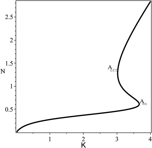
FIGURE 1. The steady state bistable curve of N against K, at fixed values of the parameters F =0.85, B =0.5. The switching-on and -off points: A_on =(3.6631,0.61299) and A_off =(3.0199,1.2793).

FIGURE 2

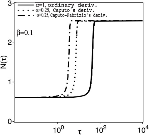
FIGURE 2. The transient population N(τ) versus the normalised time τ = γt (as log scale), for control parameter with positive perturbation, K = K_c + β; K_c =3.6631 at the switching-on point, A_on, of Figure 1 and fixed β =0.1, and for α =1 (ordinary derivative) and 0.25 (Caputo’s and Caputo-Fabrizio’s fractional derivatives).

FIGURE 3

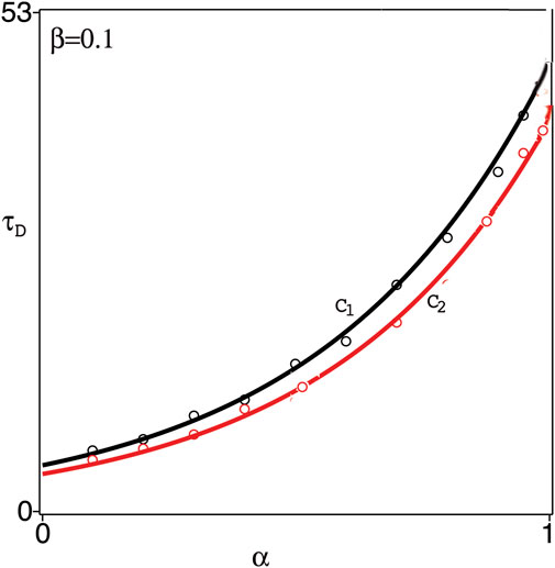
FIGURE 3. Time-delay, τ_D, versus the fractional derivative parameter α at fixed β =0.1. Circles represent the numerical results and the solid lines C₁, C₂ represent the exponential fitting, 4.9e^2.2α in the case of Caputo’s derivative, and 3.8e^2.3α in the case of Caputo-Fabrizio’s derivative, respectively.

FIGURE 4

FIGURE 4. As Figure 2, but at fixed value of α =0.25, and different β =0.01,0.3 in the case of: (A) Caputo’s, and (B) Caputo-Fabrizio’s, fractional derivatives.

FIGURE 5

FIGURE 5. Data as in Figure 2, but with negative perturbation, K_c − β at A_off, where K_c =3.0199.

In both cases of positive and negative perturbations β) at the switching-on and -off points, A_on and A_off, respectively, the time delay formula τ_D ∼|β|^−1/2 (inverse square root scaling law) essentially holds in the both cases of Caputo’s and Caputo-Fabrizio’s fractional derivatives (0 < α < 1), Figure 6, similar to the ordinary derivative case (α = 1) [14], but with different proportionality factor.

FIGURE 6

FIGURE 6. Time-delay, τ_D, versus the perturbation parameter β at the switching-on point A_on in Figure 1. Circles represent the numerical results and the dashed lines represent the corresponding fittings, $\lambda /\sqrt{\beta }$. (A) The case of ordinary derivative (α =1). (B) The case of Caputo’s fractional derivative (α =0.25). (C) As (B) but with Caputo-Fabrizio’s fractional derivative.

3.2 The Thomas reaction model

The steady state bistable curves for the Oxygen and uric acid concentrations u, v, respectively, against the supplied rate a, according to Eq. 2 or 4) are shown in Figure 7, for fixed values of other system parameters [14]. For positive perturbation β in the ordinary derivative case (α = 1) at the switching-on point, A_on in Figure 7, the transient oxygen concentration u(τ), Figure 8, shows similar qualitative behaviour of reducing τ_D in both cases of Caputo’s and Caputo-Fabrizio’s fractional derivatives, but with smaller quantitive difference. The same behaviour occurs with negative perturbation at the switching-off point A_off in Figure 7. Similar qualitative behaviour is also exhibited for the transient uric acid concentration v(t) for α = 1 [14] and α < 1. The time delay τ_D in both cases of u(τ) and v(τ) against the fractional parameter α and the perturbation parameter β shows similar qualitative behaviour as in Figures 3, 6, respectively.

FIGURE 7

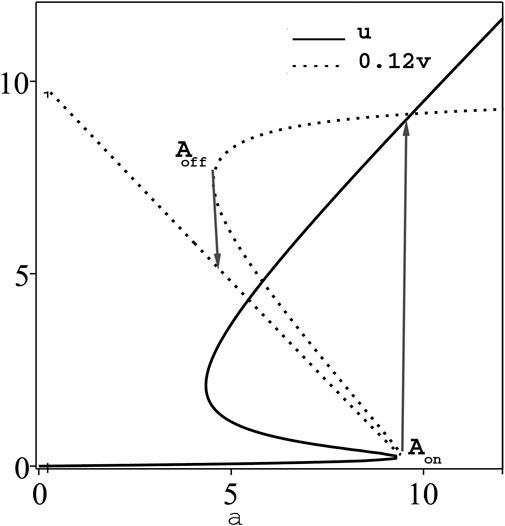
FIGURE 7. The steady state bistable curves, u and 0.12v, versus the control parameter, a, for fixed parameters K =20, B =100, γ = l =1.

FIGURE 8

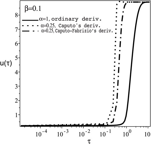
FIGURE 8. The transient Oxygen concentration, u(τ), versus the normalised time, τ with positive perturbation, κ = a_c + β, a_c =9.3643, at the switching-on point A_on of Figure 7 with fixed β =0.1 for α =1 (ordinary derivative) and 0.25 (Caputo’s and Caputo-Fabrizio’s fractional derivatives).

4 Summary

Fractional order mathematical models generalise the concept of ordinary differentiation to incorporate memory (time delay) and spatial non-local effects, and hence provide extra fractional parameters to interpret/predict the dynamical behaviour of the concerned model and capture more of its details.In this paper, we have investigated the switching time response at the critical switching-on and -off points of the bistable curves related to two biological models, namely, the spruce budworm outbreak model [3, 4, 15] and the Thomas reaction model for enzyme membrane [4, 16] within fractional order models. Two definitions of fractional derivatives of order α, (0 < α < 1) have been used, namely, Caputo’s [40] and Caputo-Fabrizio’s [21, 22] fractional derivatives. Our study shows the following.

(i) The two definitions use convolution kernels of different variability that model the memory effect, namely, as power function [40] and as exponential function [21]. Both definitions yield the same qualitative results, (ii)-(iv) below, for the two biological models referred to above. The small quantitative variance in the results is due to the different mathematical forms for the memory or delay effect.

(ii) The switching time τ_D due to the perturbation in the control (input) parameter, at the critical points of the bistable curves, is reduced further in the fractional derivative case (0 < α < 1), compared with the ordinary derivative case (α = 1) [14],

(iii) For fixed perturbation β, τ_D as a function of the fractional derivative parameter, α, (0 < α < 1) fits an exponential form, i.e., τ_D is reduced with strong memory index (α ≪ 1) and,

(iv) The switching time τ_D as a function of the perturbation parameter β fits the scaled inverse square root law $\frac{1}{\sqrt{\beta }}$ at fixed fractional derivative index (α < 1) as in the ordinary derivative case (α = 1) [14]. This is a further indication of the universality of this inverse square root law in both cases of ordinary and fractional derivative formulations. Experimental affirmation of this law in optical bistable models within ordinary derivative formation was reported in [42].

In general, fractional order models provide deeper insight into the system dynamics with memory taken, into effect and further motivate for experimental observation.Finally, we refer to some very recent works [43, 44] on biological models of COVID-19. In [43], the authors investigated various parameter estimation methods of COVID-19 incubation period using lognormal and Gamma distribution assumptions. The expressions for the maximum likelihood estimation, expectation maximisation algorithm and newly proposed algorithm [43] are termed as double or single (Riemann) integrals: these integral expressions can be converted to fractional integrals (i.e usual Riemann integral with memory or non-local, convolution kernel of fractional index, e.g. [23]), and so to have extra fractional order parameter. The other biological model of COVID-19 [44] is concerned with the stability and sensitivity analysis, and optimal control strategies of a suggested epidemic control of COVID-19. The adopted model of ODEs can be converted to FDEs and so to investigate the memory effect in this epidemic model. The formulation of the models in [43, 44] within fractional calculus will certainly add details concerning memory/non-local effects.

Data availability statement

The original contributions presented in the study are included in the article/Supplementary Material, further inquiries can be directed to the corresponding author.

Author contributions

RA: Conceptualization, Methodology, Software SH: Data curation, Writing- Original draft preparation. RA: Visualization, Investigation. SH: Supervision: RA: Software, Validation: SH: Writing- Reviewing and Editing. All authors contributed to the article and approved the submitted version.

Funding

The authors received the fund by the Deanship of Scientific Research (DSR), King Abdulaziz University, Jeddah under grant No. (G-184-247-1443).

Conflict of interest

The authors declare that the research was conducted in the absence of any commercial or financial relationships that could be construed as a potential conflict of interest.

Publisher’s note

All claims expressed in this article are solely those of the authors and do not necessarily represent those of their affiliated organizations, or those of the publisher, the editors and the reviewers. Any product that may be evaluated in this article, or claim that may be made by its manufacturer, is not guaranteed or endorsed by the publisher.

Supplementary material

The Supplementary Material for this article can be found online at: https://www.frontiersin.org/articles/10.3389/fphy.2023.1123370/full#supplementary-material

References

1. Gibbs HM. Optical bistability: Controling light with light. In: Quantum electronics-principles and applications. Massachusetts, United States: Academic Press (1985).

Google Scholar

2. Mandel P, Erneux T. Nonlinear control in optical bistability. IEEE J Quan Electron (1985) 21:1352–5. doi:10.1109/jqe.1985.1072832

CrossRef Full Text | Google Scholar

3. May RM. Thresholds and break points in ecosystems with a multiplicity of stable states. Nature (1977) 289:471–7. doi:10.1038/269471a0

CrossRef Full Text | Google Scholar

4. Murray JD. Mathematical biology: I. An introduction. 3rd ed. Berlin, Germany: Springer (2002).

Google Scholar

5. Cribier S, Giacobino E, Grynberg G. Quantitative investigation of critical slowing down in all-optical bistability. Opt Commun (1983) 47:170–2. doi:10.1016/0030-4018(83)90109-8

CrossRef Full Text | Google Scholar

6. Garmire E, Marburger JH, Allen SD, Winful HG. Transient response of hybrid bistable optical devices. Appl. Phys Lett (1979) 34:374–6.

CrossRef Full Text | Google Scholar

7. Shu Q, Rand SC. Critical slowing down and dispersion of avalanche upconversion dynamics. Phys Rev B (1997) 55:8776–83. doi:10.1103/physrevb.55.8776

CrossRef Full Text | Google Scholar

8. Boettner C, Boers N. Critical slowing down in dynamical systems driven by nonstationary correlated noise. Phys Rev Res (2022) 4:013230–7. doi:10.1103/physrevresearch.4.013230

CrossRef Full Text | Google Scholar

9. Wolchover N. Nature’s critical warning system (2015). Available at https://www.quantamagazine.org/20151117-natures-critical-warning-system/ Accessed 2015.

Google Scholar

10. Carpenter SR, Brock WA. Rising variance: A leading indicator of ecological transition. Ecol Lett (2006) 9:311–8. doi:10.1111/j.1461-0248.2005.00877.x

PubMed Abstract | CrossRef Full Text | Google Scholar

11. Dakos V, Scheffer M, van Nes EH, Brovkin V, Petoukhov V, Held H. Slowing down as an early warning signal for abrupt climate change. Proc Natl Acad Sci (2008) 105:14308–12. doi:10.1073/pnas.0802430105

PubMed Abstract | CrossRef Full Text | Google Scholar

12. Ditlevsen PD, Johnsen SJ. Tipping points: Early warning and wishful thinking. Geophys Res Lett (2010) 37:L19703. doi:10.1029/2010gl044486

CrossRef Full Text | Google Scholar

13. Chisholm RA, Filotas E. Critical slowing down as an indicator of transitions in two-species models. J Theor Biol (2009) 257:142–9. doi:10.1016/j.jtbi.2008.11.008

PubMed Abstract | CrossRef Full Text | Google Scholar

14. Alharbey RA, Nejad LAM, Lynch S, Hassan SS. Critical slowing down in biological bistable models. Int J. Pure Appl. Math. (2014) 93:581–602. doi:10.12732/ijpam.v93i4.8

CrossRef Full Text | Google Scholar

15. Ludwig D, Jones DD, Holling CS. Qualitative analysis of insect outbreak systems: The spruce budworm and forest. J Anim Ecol (1978) 47:315–32. doi:10.2307/3939

CrossRef Full Text | Google Scholar

16. Thomas D. Artificial enzyme membranes, transport, memory and oscillation. In: D Thomas, and JP Kernevez, editors. Analysis and control of immobilized enzyme systems. Berlin Heidelberg New York: Springer (1975). p. pp115–150.

Google Scholar

17. Machado JAT, Kiryakova V, Mainardi F. Recent history of fractional calculus. Commun. Nonlinear Sci Numer Simulat (2011) 16:1140–53.

CrossRef Full Text | Google Scholar

18. Du M, Wong Z, Hu H. Measuring memory with the order of fractional derivative. Scientific Rep (2013) 3:3431–3. doi:10.1038/srep03431

PubMed Abstract | CrossRef Full Text | Google Scholar

19.De Oliveira, Edmundo CapelasJos Antnio Tenreiro Machado. A review of definitions for fractional derivatives and integral. Math Probl Eng (2014) 2014:1–6. doi:10.1155/2014/238459

CrossRef Full Text | Google Scholar

20. Teodoro GS, Machado JT, De Oliveira EC. A review of definitions of fractional derivatives and other operators. J Comput Phys (2019) 388:195–208. doi:10.1016/j.jcp.2019.03.008

CrossRef Full Text | Google Scholar

21. Caputo M, Fabrizio’s M. A new definition of fractional derivative without singular kernel. Progr Fract Differ Appl (2015) 2:73–85.

Google Scholar

22. Caputo M, Fabrizio M. Applications of new time and spatial fractional derivatives with exponential kernels. Progr Fract Differ Appl (2016) 2:1–11. doi:10.18576/pfda/020101

CrossRef Full Text | Google Scholar

23. Podlubny I. Fractional differential euqations. Massachusetts, United States: Academic Press (1999).

Google Scholar

24. Caputo M, Mainardi F. A new dissipation model based on memory mechanism. Pure Appl Geophys (1971) 91:134–47. doi:10.1007/bf00879562

CrossRef Full Text | Google Scholar

25. Anastasio TJ. The fractional-order dynamics of brainstem vestibulo-oculomotor neurons. Biol Cybernet (1994) 72:69–79. doi:10.1007/bf00206239

PubMed Abstract | CrossRef Full Text | Google Scholar

26. Magin RL. Fractional calculus in engineering. USA: Begell House Publishers (2006).

Google Scholar

27. Sweilam NH, Khader MM, Mahdy AMS. Computational methods for fractional differential equations generated by optimization problem. J Fractional Calculus Appl (2012) 3:1–12.

Google Scholar

28. Tong P, Feng Y, Lv H. Euler’s method for fractional differential equations. WSEAS Transaction Maths (2013) 12:1146–53.

Google Scholar

29. Meral FC, Royston TJ, Magin R. Fractional calculus in viscoelasticity: An experimental study. Commun Nonlinear Sci Numer Simulation (2010) 15:939–45. doi:10.1016/j.cnsns.2009.05.004

CrossRef Full Text | Google Scholar

30. Xu Z, Chen W. A fractional-order model on new experiments of linear viscoelastic Creep of hami melon. Comput Maths Appl (2013) 66:677–81. doi:10.1016/j.camwa.2013.01.033

CrossRef Full Text | Google Scholar

31. Scheidegger AE, Johnson EF. The statistical behavior of instabilities in displacement processes in porous media. Can J Phys (1961) 39:326–34. doi:10.1139/p61-031

CrossRef Full Text | Google Scholar

32. Verma AP. Statistical behavior of fingering in a displacement process in heterogeneous porous medium with capillary pressure. Can J Phys (1969) 47:319–24. doi:10.1139/p69-042

CrossRef Full Text | Google Scholar

33. Bhathawala PH, Parveen S. Analytic study of three phase flow through porous media. J Indian Acad Math (2001) 23:17–24.

Google Scholar

34. Prajapati JC, Patel AD, Pathak KN, Shukla AK. Fractional calculus approach in the study of instability phenomenon in fluid dynamics. Palestine J Maths (2012) 2:95–105.

Google Scholar

35. West BJ, Turalska M. The fractional Landau model. IEEE/CAA J Automatica Sinica. (2016) 3:257–60.

Google Scholar

36. Joshi H, Jha BK. Fractional-order mathematical model for calcium distribution in nerve cells. Comput Appl Maths (2020) 39:56–22. doi:10.1007/s40314-020-1082-3

CrossRef Full Text | Google Scholar

37. Comlekoglu T, Weinberg SH. Memory in a fractional-order cardiomyocyte model alters voltage-and calcium-mediated instabilities. Commun Nonlinear Sci Numer Simulation (2020) 89:105340. doi:10.1016/j.cnsns.2020.105340

CrossRef Full Text | Google Scholar

38. Ionescu C, Lopes A, Copot D, Machado JT, Bates JH. The role of fractional calculus in modeling biological phenomena: A review. Commun Nonlinear Sci Numer Simulation (2017) 51:141–59. doi:10.1016/j.cnsns.2017.04.001

CrossRef Full Text | Google Scholar

39. Cooperputting NG. Design into turbulence. los alamos Sci Technol Mag (2009) 1663:10–5.

Google Scholar

40. Caputo M. Linear models of dissipation whose Q is almost frequency independent, Part II. J Roy Astr Soc (1967) 13:529–39.

CrossRef Full Text | Google Scholar

41. Alistair Steyn-Ross D, Steyn-Ross M. Modeling phase transition in the brain, Springer series in computational neuroscience, Springer, NewYork, NY, 2010.

Google Scholar

42. Al-Attar HA, MacKenzie HA, Firth WJ. Critical slowing-down phenomena in an InSb optically bistable etalon. JOSA B (1986) 3:1157–63. doi:10.1364/josab.3.001157

CrossRef Full Text | Google Scholar

43. Yin MZ, Zhu QW, L X. Parameter estimation of the incubation period of COVID-19 based on the doubly interval-censored data model. Nonlinear Dyn (2021) 106:1347–58. doi:10.1007/s11071-021-06587-w

PubMed Abstract | CrossRef Full Text | Google Scholar

44. L X, Hui HW, Liu F, Bai YL. Stability and optimal control strategies for a novel epidemic model of COVID-19. Nonlinear Dyn (2021) 106:1491–507. doi:10.1007/s11071-021-06524-x

PubMed Abstract | CrossRef Full Text | Google Scholar

45. Fowler AC. Mathematical models in the applied sciences. Cambridge, United Kingdom: Cambridge University Press (1997).

Google Scholar

46. Barbotin JN, Thomas D. Electron microscopic and kinetic studies dealing with an artificial enzyme membrane. Application to a cytochemical model with the horseradish peroxidase-3,3’-diaminobenzidine system. J Histochem Cytochem (1974) 11:1048–59. doi:10.1177/22.11.1048

PubMed Abstract | CrossRef Full Text | Google Scholar

47. Chan YH, Boxer SG. Model membrane systems and their applications. Curr Opin Chem Biol (2007) 11:581–7. doi:10.1016/j.cbpa.2007.09.020

PubMed Abstract | CrossRef Full Text | Google Scholar

48. Zaid M. Odibat and shaher momani, an algorithm for the numerical solution of differential equations of fractional order. J Appl Math Inform (2008) 26(1-2):15–27.

Google Scholar