The applications of symbolic computation to exact wave solutions of two HSI-like equations in (2+1)-dimensional

It is renowned that Hirota–Satsuma–Ito (HSI) equation is widely used to study wave dynamics of shallow water. In this work, two new HSI-like equations are investigated which could be extended to diversify problems in natural phenomena and give admirable contributions by applying the generalized exponential rational function method (GERFM). With the aid of symbolic calculations, various constraints on the free parameters are given, while classes of wave solutions are explicitly constructed from the coefficients of the combined non-linear and dissipative terms. After specifying values for free parameters, singular, periodic singular and anti-kink waves are demonstrated in 3D figures to exhibit different kinds of wave propagations. The fact that parameters directly influence the wave amplitude and speed of traveling waves is illustrated. The derived results are innovative and have important applications in the current field of mathematical physics research. Eventually, we show that generalized exponential rational function method is effective and straightforward to solve higher-order and high-dimensional non-linear evolution equations.

1 Introduction

It is well-known that soliton waves are normally localized in time and space, and in the field of the non-linear evolution equations (NLEEs) solitary waves are considered as the main fundamental properties. Meanwhile, the multi-soliton waves are considered as significant features to the integrable equations where the existence of soliton and multi-soliton waves is naturally used to investigate non-linear physical phenomena in the real world [1]. Recently, various versions of models have been explored, some of which are the Sawada–Kotera (SK) equation to the study of the motion of long waves in shallow water under the gravity [2], the Kadomtsev–Petviashvili (KP) equation to the study of bifurcation phenomena in fluids [3], the Hirota–Satsuma–Ito (HSI) equation to the study of shallow water wave [4–12], the Schrodinger equations to the study of fiber applications [13–15] and others [16–34]. Moreover, with the rapid development of computer calculation science, in the latest decade, many scientists have paid attention to the analytical solutions of NLEEs. In order to better understand the non-linear features in reality, it is very important to obtain exact solutions used to simulate the non-linear phenomena.

It is noted that several methods have been presented to generate the exact solutions of non-linear mathematical models through the traveling wave transformation, converting the non-linear partial differential equations (NPDEs) into ordinary differential equations (ODEs). As people known most of the proposed methods can be divided into two categories. The first one can be used to generate a limited set of exact solutions by simple computation and the second one requires complex computation, but can produce abundant wave solutions, such as the symbolic computation method [20–22, 27–34]. References [16, 17] proposed other efficient methods to deal with the complex computation issue. However, it is notable that Kudryashov [18] indicated many popular methods in finding the exact solutions are equivalent to each other. It means that although there are several published effective methods for generating exact solutions in various forms, some of them are redundant solutions. Very recently, an efficient and effective methodology, called the generalized exponential rational function method (GERFM) [20–22, 31] has been presented to extract exact solutions of the non-linear equations. After surveying the literature, it is clear to see that GERFM is a powerful methodology to handle the tough and tedious mathematical problems arising from solving high-order and high-dimensional NLEEs. With the aid of symbolic computation, complex equations solved in a single framework can be efficiently handled with GERFM. Comparing to the methods in literature, the presented method can effectively yield multiple wave solutions instead of equivalent solutions. It is well known that the study of exact solutions of NLEEs has plays a pivotal role in understating the non-linear physical phenomena. In this research, the derived results are innovative, and therefore, have important applications in the current field of mathematical physics research.

In the past two decades integrable equations play an important role in simulating complex physical phenomena [1]. To be one of integrable equations the HSI equation is considerable to characterize the (2+1)-dimensional interaction of waves in terms of dissipative effect in fluid mechanics. Accordingly, HSI is an important one used in the study of the propagation of shallow-water waves in non-linear systems. As a consequence, we may trust that the investigation of the HSI equation is able to further explore the diverse physical phenomena in non-linear science, such as the reported works [32–34] given the lump and Pfaffian form solutions.

On the other hand, the mathematical modeling of countless physical systems has implications for NLEEs in various fields of applied science and engineering. Fortunately, two newly constructed (2+1)-dimensional HIS-like equations were proposed [9] constructed as

$\alpha \left[3{\left(u_x{u}_t\right)}_x+u_{xxxt}\right]+{\delta }_1{u}_{yt}+{\delta }_2{u}_{xx}=0,$(1.1)

and

$\alpha \left[3{\left(u_x{u}_t\right)}_x+u_{xxxt}\right]+\beta \left[3{\left(u_x{u}_y\right)}_x+u_{xxxy}\right]+{\delta }_3{u}_{xx}+{\delta }_4{u}_{xy}+{\delta }_5{u}_{yy}=0,$(1.2)

where the study of the resonance Y-type multi-soliton solutions and soliton molecules were achieved. The research results can be utilized to better describe a variety of physical phenomena and understand the inelastic interactions of wave propagating in shallow-water wave and the related field of Jimbo–Miwa (JM) classification [9]. As mentioned above, more and more accurate solutions will be of great help to scientists to further study traveling waves in non-linear fluids. However, the correspondingly traveling wave solutions to the above equations have hitherto been unreported. Thus, in order to make more contributions to the study of traveling wave, the above two equations are examined by GERFM.

A class of new and different solutions including periodic and Anti-kink waves are explicitly constructed from the coefficients of combined non-linear and dissipative terms via symbolic calculations. The rest sections of this work are as follows. In Section 2, the algorithms of GERFM are illustrated step by step. In Section 3, a variety of exact solutions to above equations are formally generated and simulated in 3D figures. Meanwhile, the characteristics of traveling waves are elaborated in detail. Finally, the conclusion is given.

2 Methodology

GERFM is a relatively novel methodology to handle the partial differential equations by utilizing the wave transformation to transform the examined NPDEs into ODEs. To illustrate the method, let us consider a NPDE in the form:

$\mathrm{L}\left(\psi ,{\psi }_x,{\psi }_t,{\psi }_{xx},\dots \right)=0.$(2.1)

Firstly, via taking into account the new variable of $\xi =\kappa x+\mu y+\omega t$, Eq. 2.1 can be turned to the non-linear ODE as

$L\left(\psi \left(\xi \right),\frac{d\psi }{d\xi },\frac{d^2\psi }{d{\xi }^2},...\right)=0,$(2.2)

where $k,\mu ,\omega$ are some undetermined parameters that are determined during the procedure.

Step 2. Assume that Eq. 2.2 has the solution constructed as

$\psi \left(\xi \right)=A_0+{\displaystyle \sum }_{i=1}^M{A}_i{\left(\frac{\mathrm{\Phi }\left(\xi \right)}{{\mathrm{\Phi }}^{\prime }\left(\mathrm{\xi }\right)}\right)}^i+{\displaystyle \sum }_{i=1}^M{B}_k{\left(\frac{\mathrm{\Phi }\left(\xi \right)}{{\mathrm{\Phi }}^{\prime }\left(\xi \right)}\right)}^{-i},$(2.3)

where

$\mathrm{\Phi }\left(\xi \right)=\frac{p_1\exp \left(q_1\xi \right)+p_2\exp \left(q_2\xi \right)}{p_3\exp \left(q_3\xi \right)+p_4\exp \left(q_4\xi \right)}.$(2.4)

The value of $M$ in Eq. 2.3 is yield via the balance principle [1] and the unknown parameter $p_j,q_j\left(1\le j\le 4\right),A_0,\dots ,A_i$ and $B_i\left(1\le i\le M\right)$ will be determined by the examined Eq. 2.2.

Step 3. Following the above steps Eq. 2.3 will satisfy Eq. 2.2. Then, putting Eq. 2.3 into Eq. 2.2 yields a system of non-linear equations. Then, with the aid of the symbolic computation software such as Maple, the values of $p_i,q_i\left(1\le i\le 4\right),A_0,\dots ,A_k$, and $B_k\left(1\le k\le M\right)$ are determined. Finally, by using Eq. 2.3 various versions of exact solutions to Eq. 2.1 are extracted.

3 Two new HSI-like equations

In this section, we will exert the GERFM to obtain the wave solutions to Eq. 1.1 and Eq. 1.2, including periodic wave, solitary wave and others.

3.1 The solutions to Eq. 1.1

Via wave transformation $\xi =\kappa x+\mu y+\omega t$ along with $U\left(\xi \right)=u\left(x,y,z,t\right)$ Eq. 1.1 is transformed into an ODE as

$\left(\frac{d^2}{d{\xi }^2}U\right)\left(6\alpha {\kappa }^2\omega \left(\frac{d}{d\xi }U\right)+\mu \omega {\delta }_1+{\delta }_2{\kappa }^2\right)+\alpha {\kappa }^3\omega \left(\frac{d^4}{d{\xi }^4}U\right)=0,$(3.1)

and integrating Eq. 3.1, once yields

$3\alpha {\kappa }^2\omega {\left(\frac{d}{d\xi }U\right)}^2+{\delta }_2{\kappa }^2\left(\frac{d}{d\xi }U\right)+\mu \omega {\delta }_1\left(\frac{d}{d\xi }U\right)+\alpha {\kappa }^3\omega \left(\frac{d^3}{d{\xi }^3}U\right)=0.$(3.2)

Now, Eq. 3.2 is ready to be handled by GERFM.

Via the balancing principle between ${U_{\xi }}^2$ and $U_{\xi \xi \xi }$ in Eq. 3.2, we get $M=1$. Hence, from Eq. 2.3, the solution form will be constructed as

$u\left(\xi \right)=A_0+A_1\left(\frac{\mathrm{\Phi }\left(\xi \right)}{{\mathrm{\Phi }}^{\prime }\left(\xi \right)}\right)+B_1{\left(\frac{\mathrm{\Phi }\left(\xi \right)}{{\mathrm{\Phi }}^{\prime }\left(\xi \right)}\right)}^{-1}.$(3.3)

Based on the algorithms in Section 2, several different kinds of resolutions are accordingly derived as follows.

Category 1: Taking into account $p=\left[-3,-\mathrm{1,1,1}\right]$ and $q=\left[1,-\mathrm{1,1},-1\right]$ gives

$\mathrm{\Phi }\left(\xi \right)=\frac{-\sinh \left(\xi \right)-2\cosh \left(\xi \right)}{\cosh \left(\xi \right)}.$(3.4)

and the several different sets of resolutions as follows.

Set 1:

$\omega =-\frac{{\kappa }^2{\delta }_2}{4\alpha {\kappa }^3+{\delta }_1\mu },A_1=0,B_1=6\kappa ,$(3.5)

where $A_0,\kappa ,\mu$ are arbitrary contents.

Substituting the values of the parameters Eq. 3.5 into Eq. 3.3 and Eq. 3.4, one obtains the following wave solution as

$U\left(\xi \right)=\frac{\left(-6\kappa +2A_0\right)\cosh \left(\xi \right)+A_0\sinh \left(\xi \right)}{\sinh \left(\xi \right)+2\cosh \left(\xi \right)}.$(3.6)

Thereupon, Eq. 1.1 admits the following exact solution

$u_{\mathrm{1,1}}\left(x,y,t\right)=\frac{\left(-6\kappa +2A_0\right)\cosh \left(\kappa x+\mu y-\frac{{\kappa }^2{\delta }_2}{4\alpha {\kappa }^3+{\delta }_1\mu }t\right)+A_0\sinh \left(\kappa x+\mu y-\frac{{\kappa }^2{\delta }_2}{4\alpha {\kappa }^3+{\delta }_1\mu }t\right)}{\sinh \left(\kappa x+\mu y-\frac{{\kappa }^2{\delta }_2}{4\alpha {\kappa }^3+{\delta }_1\mu }t\right)+2\cosh \left(\kappa x+\mu y-\frac{{\kappa }^2{\delta }_2}{4\alpha {\kappa }^3+{\delta }_1\mu }t\right)}.$(3.7)

Numerical simulation corresponding to the solution $u_{\mathrm{1,1}}\left(x,y=1,t\right)$ while taking $\kappa =0.1,\mu =0.2,\alpha =0.5,{\delta }_1=1,{\delta }_2=0.5,A_0=0.5$, which is an anti-kink type solution, is presented in Figure 1.

FIGURE 1

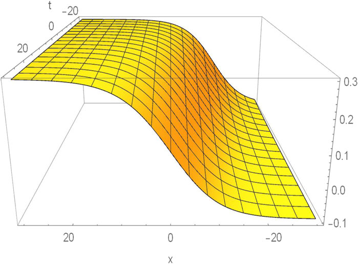
FIGURE 1. Numerical simulation of $u_{\mathrm{1,1}}\left(x,y=1,t\right)$.

Set 2:

$\omega =-\frac{{\kappa }^2{\delta }_2}{4\alpha {\kappa }^3+{\delta }_1\mu },A_1=-2\kappa ,B_1=0,$(3.8)

where $A_0,\kappa ,\mu$ are arbitrary contents.

Substituting the values of the parameters Eq. 3.8 into Eq. 3.3 and Eq. 3.4, one obtains the following wave solution as

$U\left(\xi \right)=\frac{\left(4\kappa +A_0\right)\cosh \left(\xi \right)+2\kappa \sinh \left(\xi \right)}{\cosh \left(\xi \right)}.$(3.9)

Thereupon, Eq. 1.1 admits the following exact solution

$u_{\mathrm{1,2}}\left(x,y,t\right)=\frac{\left(4\kappa +A_0\right)\cosh \left(\kappa x+\mu y-\frac{{\kappa }^2{\delta }_2}{4\alpha {\kappa }^3+{\delta }_1\mu }t\right)+2\kappa \sinh \left(\kappa x+\mu y-\frac{{\kappa }^2{\delta }_2}{4\alpha {\kappa }^3+{\delta }_1\mu }t\right)}{\cosh \left(\kappa x+\mu y-\frac{{\kappa }^2{\delta }_2}{4\alpha {\kappa }^3+{\delta }_1\mu }t\right)}.$(3.10)

Category 2: Taking into account $p=\left[\mathrm{1,0,1,1}\right]$ and $q=\left[\mathrm{1,0,1,0}\right]$, one achieves that

$\mathrm{\Phi }\left(\xi \right)=\frac{\exp \left(\xi \right)}{1+\exp \left(\xi \right)}.$(3.11)

Set 1:

$\omega =-\frac{{\kappa }^2{\delta }_2}{\alpha {\kappa }^3+{\delta }_1\mu },A_1=2\kappa ,B_1=0,$(3.12)

where $A_0,\kappa ,\mu$ are arbitrary contents.

Substituting the values of the parameters Eq. 3.12 into Eq. 3.11 and Eq. 3.3, one obtains the following kink wave as

$U\left(\xi \right)=\frac{A_0+\left(2\kappa +A_0\right)\exp \left(\xi \right)}{1+\exp \left(\xi \right)}.$(3.13)

There upon, Eq. 1.1 admits the following exact solution

$u_{\mathrm{1,3}}\left(x,y,t\right)=\frac{A_0+\left(2\kappa +A_0\right)\exp \left(\kappa x+\mu y-\frac{{\kappa }^2{\delta }_2}{\alpha {\kappa }^3+{\delta }_1\mu }t\right)}{1+\exp \left(\kappa x+\mu y-\frac{{\kappa }^2{\delta }_2}{\alpha {\kappa }^3+{\delta }_1\mu }t\right)}.$(3.14)

Numerical simulation corresponding to the solution $u_{\mathrm{1,3}}\left(x,y=1,t\right)$ while taking $\kappa =0.6,\mu =0.5,\alpha =0.9,{\delta }_1=0.8,{\delta }_2=0.1,A_0=0.5$, which is an anti-kink type solution, is presented in Figure 2.

FIGURE 2

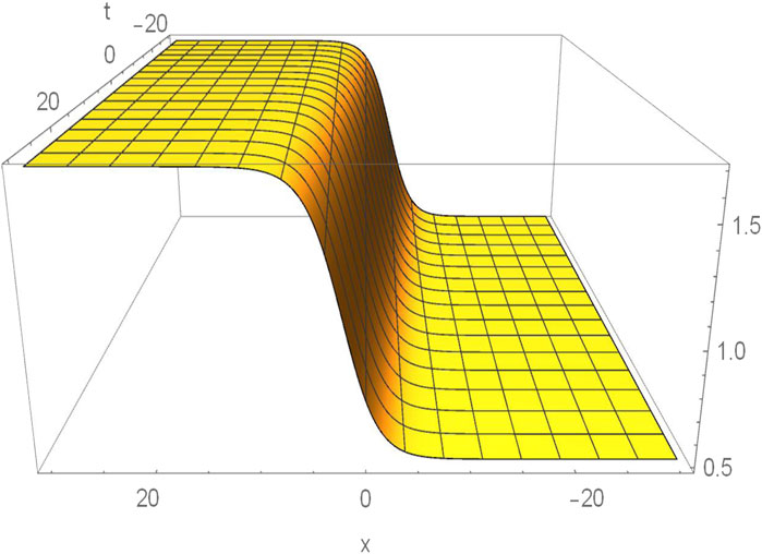
FIGURE 2. Numerical simulation of $u_{\mathrm{1,3}}\left(x,y=1,t\right)$.

Category 3: Taking into account $p=\left[1+i,1-i,\mathrm{1,1}\right]$ and $q=\left[i,-i,i,-i\right]$, one achieves that

$\mathrm{\Phi }\left(\xi \right)=\frac{-\sin \left(\xi \right)+\cos \left(\xi \right)}{\cos \left(\xi \right)}.$(3.15)

Set 1:

$\omega =-\frac{{\kappa }^2{\delta }_2}{-4\alpha {\kappa }^3+{\delta }_1\mu },A_1=2\kappa ,B_1=0,$(3.16)

where $A_0,\kappa ,\mu$ are arbitrary contents.

Substituting the values of the parameters Eq. 3.16 into Eq. 3.15 and Eq. 3.3, one obtains the following periodic wave as

$U\left(\xi \right)=\frac{\left(2\kappa +A_0\right)\cos \left(\xi \right)-2\kappa \sin \left(\xi \right)}{\cos \left(\xi \right)}.$(3.17)

Thereupon, Eq. 1.1 admits the following exact solution

$u_{\mathrm{1,4}}\left(x,y,t\right)=\frac{\left(2\kappa +A_0\right)\cos \left(\kappa x+\mu y-\frac{{\kappa }^2{\delta }_2}{-4\alpha {\kappa }^3+{\delta }_1\mu }t\right)-2\kappa \sin \left(\kappa x+\mu y-\frac{{\kappa }^2{\delta }_2}{-4\alpha {\kappa }^3+{\delta }_1\mu }t\right)}{\cos \left(\kappa x+\mu y-\frac{{\kappa }^2{\delta }_2}{-4\alpha {\kappa }^3+{\delta }_1\mu }t\right)}.$(3.18)

Numerical simulation corresponding to the solution $u_{\mathrm{1,4}}\left(x,y=1,t\right)$ while taking $\kappa =0.6,\mu =0.5,\alpha =0.9,{\delta }_1=0.8,{\delta }_2=0.1,A_0=0.5$, which is a periodic singular solution, is presented in Figure 3.

FIGURE 3

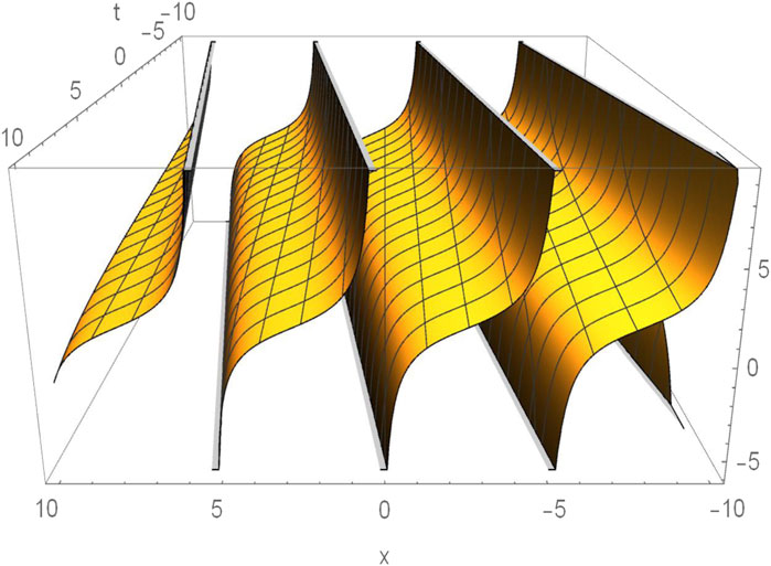
FIGURE 3. Numerical simulation of $u_{\mathrm{1,4}}\left(x,y=1,t\right)$.

Category 4: Taking into account $p=\left[1-i,1+i,\mathrm{1,1}\right]$ and $q=\left[i,-i,i,-i\right]$, one achieves that

$\mathrm{\Phi }\left(\xi \right)=\frac{\cos \left(\xi \right)+\sin \left(\xi \right)}{\cos \left(\xi \right)}.$(3.19)

Set 1:

$\omega =-\frac{{\kappa }^2{\delta }_2}{-4\alpha {\kappa }^3+{\delta }_1\mu },A_1=0,B_1=4\kappa ,$(3.20)

where $A_0,\kappa ,\mu$ are arbitrary contents.

Substituting the values of the parameters Eq. 3.20 into Eq. 3.19 and Eq. 3.3, one obtains the following periodic wave as

$U\left(\xi \right)=\frac{\left(4\kappa +A_0\right)\cos \left(\xi \right)+A_0\sin \left(\xi \right)}{\cos \left(\xi \right)+\sin \left(\xi \right)}.$(3.21)

Thereupon, Eq. 1.1 admits the following exact solution

$u_{\mathrm{1,5}}\left(x,y,t\right)=\frac{\left(4\kappa +A_0\right)\cos \left(\kappa x+\mu y-\frac{{\kappa }^2{\delta }_2}{-4\alpha {\kappa }^3+{\delta }_1\mu }t\right)+A_0\sin \left(\kappa x+\mu y-\frac{{\kappa }^2{\delta }_2}{-4\alpha {\kappa }^3+{\delta }_1\mu }t\right)}{\cos \left(\kappa x+\mu y-\frac{{\kappa }^2{\delta }_2}{-4\alpha {\kappa }^3+{\delta }_1\mu }t\right)+\sin \left(\kappa x+\mu y-\frac{{\kappa }^2{\delta }_2}{-4\alpha {\kappa }^3+{\delta }_1\mu }t\right)}.$(3.22)

Numerical simulation corresponding to the solution $u_{\mathrm{1,5}}\left(x,y=1,t\right)$ while taking $\kappa =1,\mu =1.2,\alpha =0.3,{\delta }_1=0.8,{\delta }_2=0.7,A_0=0.7$, which is a periodic singular solution, is presented in Figure 4.

FIGURE 4

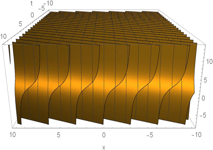
FIGURE 4. Numerical simulation of $u_{\mathrm{1,5}}\left(x,y=1,t\right)$.

Category 5: Taking into account $p=\left[-2-i,2-i,-\mathrm{1,1}\right]$ and $q=\left[i,-i,i,-i\right]$, one achieves that

$\mathrm{\Phi }\left(\xi \right)=\frac{\cos \left(\xi \right)+2\sin \left(\xi \right)}{\sin \left(\xi \right)}.$(3.23)

Set 1:

$\omega =-\frac{{\kappa }^2{\delta }_3}{-4\alpha {\kappa }^3+{\delta }_1\mu },A_1=2\kappa ,B_1=0.$(3.24)

where $A_0,\kappa ,\mu$ are arbitrary contents.

Substituting the values of the parameters Eq. 3.24 into Eq. 3.23 and Eq. 3.3, one obtains the following wave solution as

$U\left(\xi \right)=\frac{\left(4\kappa +A_0\right)\sin \left(\xi \right)+2\kappa \cos \left(\xi \right)}{\sin \left(\xi \right)}.$(3.25)

Thereupon, Eq. 1.1 admits the following exact solution

$u_{\mathrm{1,6}}\left(x,y,t\right)=\frac{\left(4\kappa +A_0\right)\sin \left(\kappa x+\mu y-\frac{{\kappa }^2{\delta }_2}{-4\alpha {\kappa }^3+{\delta }_1\mu }t\right)+2\kappa \cos \left(\kappa x+\mu y-\frac{{\kappa }^2{\delta }_2}{-4\alpha {\kappa }^3+{\delta }_1\mu }t\right)}{\sin \left(\kappa x+\mu y-\frac{{\kappa }^2{\delta }_2}{-4\alpha {\kappa }^3+{\delta }_1\mu }t\right)}.$(3.26)

Category 6: Taking into account $p=\left[-\mathrm{1,3,1},-1\right]$ and $q=\left[1,-\mathrm{1,1},-1\right]$, one achieves that

$\mathrm{\Phi }\left(\xi \right)=\frac{\cosh \left(\xi \right)-2\sinh \left(\xi \right)}{\sinh \left(\xi \right)}.$(3.27)

Set 1:

$\omega =-\frac{{\kappa }^2{\delta }_2}{4\alpha {\kappa }^3+{\delta }_1\mu },A_1=2\kappa ,B_1=0.$(3.28)

where $A_0,\kappa ,\mu$ are arbitrary contents.

Substituting the values of the parameters Eq. 3.28 into Eq. 3.27 and Eq. 3.3, one obtains the following wave solution as

$U\left(\xi \right)=\frac{\left(-4\kappa +A_0\right)\sinh \left(\xi \right)+2\kappa \cosh \left(\xi \right)}{\sinh \left(\xi \right)}.$(3.29)

Thereupon, Eq. 1.1 admits the following exact solution

$u_{\mathrm{1,7}}\left(x,y,t\right)=\frac{\left(-4\kappa +A_0\right)\sinh \left(\kappa x+\mu y-\frac{{\kappa }^2{\delta }_{2}t}{4\alpha {\kappa }^3+{\delta }_1\mu }\right)+2\kappa \cosh \left(\kappa x+\mu y-\frac{{\kappa }^2{\delta }_{2}t}{4\alpha {\kappa }^3+{\delta }_1\mu }\right)}{\sinh \left(\kappa x+\mu y-\frac{{\kappa }^2{\delta }_{2}t}{4\alpha {\kappa }^3+{\delta }_1\mu }\right)}.$(3.30)

Numerical simulation corresponding to the solution $u_{\mathrm{1,7}}\left(x,y=1,t\right)$ while taking $\kappa =1,\mu =1.2,\alpha =0.8,{\delta }_1=0.2,{\delta }_2=0.3,A_0=0.7$, which is a singular solution, is presented in Figure 5.

FIGURE 5

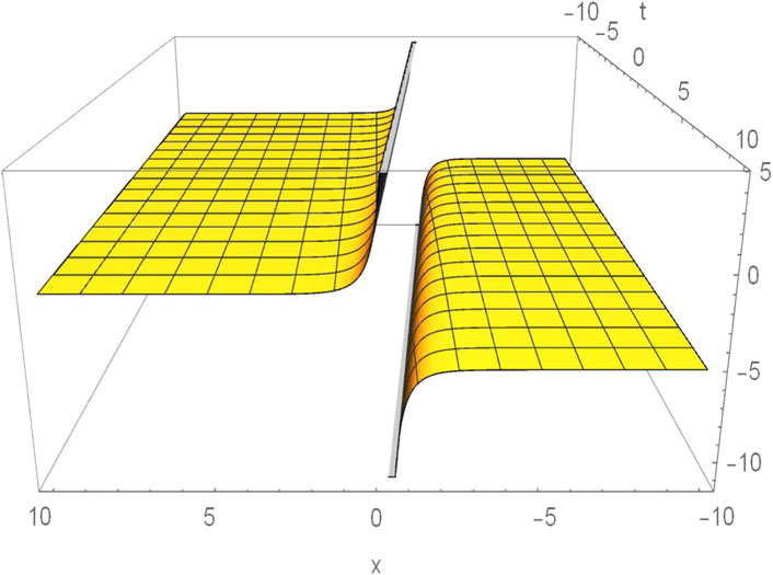
FIGURE 5. Numerical simulation of $u_{\mathrm{1,7}}\left(x,y=1,t\right)$.

Category 7: Taking into account $p=\left[i,-i,\mathrm{1,1}\right]$ and $q=\left[i,-i,i,-i\right]$, one achieves that

$\mathrm{\Phi }\left(\xi \right)=-\frac{\sin \left(\xi \right)}{\cos \left(\xi \right)}.$(3.31)

Set 1:

$\kappa =-\frac{B_1}{2},\mu =-\frac{B_1^2\left(8B_1\omega \alpha +{\delta }_2\right)}{4{\delta }_1\omega },A_1=-B_1,$(3.32)

where $A_0,B_1,\omega$ are arbitrary contents.

Substituting the values of the parameters Eq. 3.32 into Eq. 3.31 and Eq. 3.3, one obtains the following periodic wave as

$U\left(\xi \right)=\frac{-4B_1{\cos }^2\left(\xi \right)+A_0\sin \left(2\xi \right)+2B_1}{\sin \left(2\xi \right)}.$(3.33)

Thereupon, Eq. 1.1 admits the following exact solution

$u_{\mathrm{1,8}}\left(x,y,t\right)=\frac{-4B_1{\cos }^2\left(\xi \right)+A_0\sin \left(2\xi \right)+2B_1}{\sin \left(2\xi \right)},$(3.34)

where

$\xi =-B_{1}x-\frac{B_1^2\left(8B_1\omega \alpha +{\delta }_2\right)}{2{\delta }_1\omega }y+2\omega t.$(3.35)

Numerical simulation corresponding to the solution $u_{\mathrm{1,8}}\left(x,y=1,t\right)$ while taking $\kappa =1,\mu =0.8,\alpha =0.8,{\delta }_1=0.7,{\delta }_2=0.3,\omega =0.3,A_0=0.7,B_1=0.7$, which is a periodic singular solution, is presented in Figure 6.

FIGURE 6

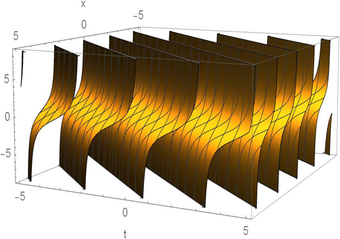
FIGURE 6. Numerical simulation of $u_{\mathrm{1,8}}\left(x,y=1,t\right)$.

Category 8: Taking into account $p=\left[1,-\mathrm{1,1},-1\right]$ and $q=\left[1,-\mathrm{1,1},-1\right]$, one achieves that

$\mathrm{\Phi }\left(\xi \right)=-\frac{\cosh \left(\xi \right)}{\sinh \left(\xi \right)}.$(3.36)

Set 1:

$\kappa =-\frac{B_1}{2},\mu =\frac{B_1^2\left(8B_1\omega \alpha -{\delta }_2\right)}{4{\delta }_1\omega },A_1=B_1,$(3.37)

where $A_0,B_1,\omega$ are arbitrary contents.

Substituting the values of the parameters Eq. 3.37 into Eq. 3.36 and Eq. 3.3, one obtains the following wave solution as

$U\left(\xi \right)=\frac{-B_1{\coth }^2\left(\xi \right)+A_0\coth \left(\xi \right)-B_1}{\coth \left(\xi \right)}.$(3.38)

Thereupon, admits the following exact solution

$u_{\mathrm{1,9}}\left(x,y,t\right)=\frac{-B_1{\coth }^2\left(\xi \right)+A_0\coth \left(\xi \right)-B_1}{\coth \left(\xi \right)},$(3.39)

Where

$\xi =-\frac{B_{1}x}{2}+\frac{B_1^2\left(8B_1\omega \alpha -{\delta }_2\right)y}{4{\delta }_1\omega }+\omega t.$(3.40)

Category 9: Taking into account $p=\left[-\mathrm{1,1,1,1}\right]$ and $q=\left[1,-\mathrm{1,1},-1\right]$, one achieves that

$\mathrm{\Phi }\left(\xi \right)=-\frac{\sinh \left(\xi \right)}{\cosh \left(\xi \right)}.$(3.41)

Set 1:

$\kappa =-\frac{A_1}{2},\mu =\frac{A_1^2\left(2\alpha \omega A_1-{\delta }_2\right)}{4{\delta }_1\omega },B_1=0,$(3.42)

where $A_0,A_1,\omega$ are arbitrary contents.

Substituting the values of the parameters Eq. 3.42 into Eq. 3.41 and Eq. 3.3, one obtains the following kink wave as

$U\left(\xi \right)=A_0-A_1\tanh \left(\xi \right).$(3.43)

Thereupon, Eq. 1.1 admits the following exact solution

$u_{\mathrm{1,10}}\left(x,y,t\right)=A_0-A_1\tanh \left(-\frac{A_{1}x}{2}+\frac{A_1^2\left(2\alpha \omega A_1-{\delta }_2\right)y}{4{\delta }_1\omega }+\omega t\right).$(3.44)

Numerical simulation corresponding to the solution $u_{\mathrm{1,10}}\left(x,y=1,t\right)$ while taking $\kappa =1,\mu =0.8,\alpha =0.6,{\delta }_1=0.5,{\delta }_2=0.3,\omega =0.9,A_0=0.1,A_1=0.7$, which is an anti-kink type solution, is presented in Figure 7.

FIGURE 7

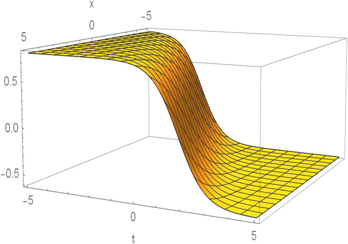
FIGURE 7. Numerical simulation of $u_{\mathrm{1,10}}\left(x,y=1,t\right)$.

Category 10: Taking into account $p=\left[\mathrm{1,1},-\mathrm{1,1}\right]$ and $q=\left[1,-\mathrm{1,1},-1\right]$, one achieves that

$\mathrm{\Phi }\left(\xi \right)=\frac{\cosh \left(\xi \right)}{\sinh \left(\xi \right)}.$(3.45)

Set 1:

$\kappa =\frac{B_1}{2},\mu =-\frac{B_1^2\left(8B_1\omega \alpha +{\delta }_2\right)}{4{\delta }_1\omega },A_1=B_1,$(3.46)

where $A_0,B_1,\omega$ are arbitrary contents.

Substituting the values of the parameters Eq. 3.46 into Eq. 3.45 and Eq. 3.3, one obtains the following wave solution as

$U\left(\xi \right)=\frac{2B_1{\cosh }^2\left(\xi \right)+A_0\sinh \left(2\xi \right)-B_1}{\sinh \left(2\xi \right)}.$(3.47)

Thereupon, Eq. 1.1 admits the following exact solution

$u_{\mathrm{1,11}}\left(x,y,t\right)=\frac{2B_1{\cosh }^2\left(\xi \right)+A_0\sinh \left(2\xi \right)-B_1}{\sinh \left(2\xi \right)}.$(3.48)

where

$\xi =B_{1}x-\frac{B_1^2\left(8B_1\omega \alpha +{\delta }_2\right)y}{2{\delta }_1\omega }+\omega t.$(3.49)

So far, via the appropriate choice of free parameters there has 11 exact solutions are formally presented to Eq. 1.1 which are valuable to demonstrate the propagation of traveling waves.

3.2 The solutions for Eq. 1.2

In this section, we will exert the GERFM to obtain the wave solutions to Eq. 1.2 including periodic wave, solitary wave and others.

Via the mentioned algorithm Eq. 1.2 is transformed into an ODE as

$\alpha {\kappa }^3\omega \left(\frac{d^4}{d{\xi }^4}U\right)+\left(\frac{d^2}{d{\xi }^2}U\right)\times \left(6{\kappa }^2\left(\alpha \omega +\beta \mu \right)\left(\frac{d}{d\xi }U\right)+{\mu }^2{\delta }_5+\mu {\delta }_4\kappa +{\delta }_3{\kappa }^2\right)=0.$(3.50)

Then, integrating Eq. 3.50 once yields

$\alpha {\kappa }^3\omega \left(\frac{d^3}{d{\xi }^3}U\right)+\left(3\alpha {\kappa }^2\omega +3\beta {\kappa }^2\mu \right){\left(\frac{d}{d\xi }U\right)}^2+\left({\delta }_3{\kappa }^2+\mu {\delta }_4\kappa +{\mu }^2{\delta }_5\right)\left(\frac{d}{d\xi }U\right)=0.$(3.51)

Now, Eq. 3.51 is the perfect form to be handled by GERFM and used to retrieve a variety of wave solutions to Eq. 1.2. It is noted that employing the balancing principle in Eq. 3.51 gives $M=1$. Hence, from Eq. 2.3, the solution of Eq. 3.51 will be constructed as same as Eq. 3.3. Then, proceeding as before we get the following solutions:

Category 1: Taking into account $p=\left[\mathrm{1,1},-\mathrm{1,1}\right]$ and $q=\left[1,-\mathrm{1,1},-1\right]$, one achieves that

$\mathrm{\Phi }\left(\xi \right)=-\frac{\cosh \left(\xi \right)}{\sinh \left(\xi \right)}.$(3.52)

Set 1:

$\omega =\frac{-{\kappa }^2{\delta }_3-\mu {\delta }_4\kappa -{\mu }^2{\delta }_5}{16\alpha {\kappa }^3},A_1=B_1=-\frac{2\left({\kappa }^2{\delta }_3+\mu {\delta }_4\kappa +{\mu }^2{\delta }_5\right)\kappa }{-16\beta {\kappa }^3\mu +{\kappa }^2{\delta }_3+\mu {\delta }_4\kappa +{\mu }^2{\delta }_5},$(3.53)

where $\kappa ,\mu ,A_0$ are arbitrary contents.

Substituting the values of the parameters Eq. 3.53 into Eq. 3.52 and Eq. 3.3, one obtains the following wave solution as

$U\left(\xi \right)=\frac{\left(\begin{array}{l}2{\mu }^2{\delta }_5\kappa +2\mu {\delta }_4{\kappa }^2+2{\kappa }^3{\delta }_3+\left(2{\kappa }^3{\delta }_3+2\mu {\delta }_4{\kappa }^2+2{\mu }^2{\delta }_5\kappa \right){\coth }^2\left(\xi \right)\\ +A_0\left(-16\beta {\kappa }^3\mu +{\kappa }^2{\delta }_3+\mu {\delta }_4\kappa +{\mu }^2{\delta }_5\right)\coth \left(\xi \right)\end{array}\right)}{\left(-16\beta {\kappa }^3\mu +{\kappa }^2{\delta }_3+\mu {\delta }_4\kappa +{\mu }^2{\delta }_5\right)\coth \left(\xi \right)}.$(3.54)

Thereupon, Eq. 1.2 admits the following exact solution

$u_{\mathrm{2,1}}\left(x,y,t\right)=\frac{\left(\begin{array}{l}2{\mu }^2{\delta }_5\kappa +2\mu {\delta }_4{\kappa }^2+2{\kappa }^3{\delta }_3+\left(2{\kappa }^3{\delta }_3+2\mu {\delta }_4{\kappa }^2+2{\mu }^2{\delta }_5\kappa \right){\coth }^2\left(\xi \right)\\ +A_0\left(-16\beta {\kappa }^3\mu +{\kappa }^2{\delta }_3+\mu {\delta }_4\kappa +{\mu }^2{\delta }_5\right)\coth \left(\xi \right)\end{array}\right)}{\left(-16\beta {\kappa }^3\mu +{\kappa }^2{\delta }_3+\mu {\delta }_4\kappa +{\mu }^2{\delta }_5\right)\coth \left(\xi \right)},$(3.55)

where

$\xi =\kappa x+\mu y+\frac{\left(-{\kappa }^2{\delta }_3-\mu {\delta }_4\kappa -{\mu }^2{\delta }_5\right)}{16\alpha {\kappa }^3}t.$(3.56)

Set 2:

$\omega =\frac{-{\kappa }^2{\delta }_3-\mu {\delta }_4\kappa -{\mu }^2{\delta }_5}{4\alpha {\kappa }^3},A_1=-\frac{2\left({\kappa }^2{\delta }_3+\mu {\delta }_4\kappa +{\mu }^2{\delta }_5\right)\kappa }{-4\beta {\kappa }^3\mu +{\kappa }^2{\delta }_3+\mu {\delta }_4\kappa +{\mu }^2{\delta }_5},B_1=0,$(3.57)

where $\kappa ,\mu ,A_0$ are arbitrary contents.

Substituting the values of the parameters Eq. 3.57 into Eq. 3.52 and Eq. 3.3, one obtains the following wave solution as

$U\left(\xi \right)=\frac{\left(2{\kappa }^3{\delta }_3+2\mu {\delta }_4{\kappa }^2+2{\mu }^2{\delta }_5\kappa \right)\coth \left(\xi \right)+A_0\left(-4\beta {\kappa }^3\mu +{\kappa }^2{\delta }_3+\mu {\delta }_4\kappa +{\mu }^2{\delta }_5\right)}{-4\beta {\kappa }^3\mu +{\kappa }^2{\delta }_3+\mu {\delta }_4\kappa +{\mu }^2{\delta }_5}.$(3.58)

Thereupon, Eq. 1.2 admits the following exact solution

$u_{\mathrm{2,2}}\left(x,y,t\right)=\frac{\left(\begin{array}{l}\left(2{\kappa }^3{\delta }_2+2\mu {\delta }_4{\kappa }^2+2{\mu }^2{\delta }_5\kappa \right)\coth \left(\kappa x+\mu y+\frac{\left(-{\kappa }^2{\delta }_3-\mu {\delta }_4\kappa -{\mu }^2{\delta }_5\right)}{4\alpha {\kappa }^3}t\right)\\ +A_0\left(-4\beta {\kappa }^3\mu +{\kappa }^2{\delta }_3+\mu {\delta }_4\kappa +{\mu }^2{\delta }_5\right)\end{array}\right)}{-4\beta {\kappa }^3\mu +{\kappa }^2{\delta }_3+\mu {\delta }_4\kappa +{\mu }^2{\delta }_5}.$(3.59)

Set 3:

$\omega =\frac{-{\kappa }^2{\delta }_3-\mu {\delta }_4\kappa -{\mu }^2{\delta }_5}{4\alpha {\kappa }^3},A_1=0,B_1=-\frac{2\left({\kappa }^2{\delta }_3+\mu {\delta }_4\kappa +{\mu }^2{\delta }_5\right)\kappa }{-4\beta {\kappa }^3\mu +{\kappa }^2{\delta }_3+\mu {\delta }_4\kappa +{\mu }^2{\delta }_5},$(3.60)

where $\kappa ,\mu ,A_0$ are arbitrary contents.

Substituting the values of the parameters Eq. 3.60 into Eq. 3.52 and Eq. 3.3, one obtains the following wave solution as

$U\left(\xi \right)=\frac{A_0\left(-4\beta {\kappa }^3\mu +{\kappa }^2{\delta }_3+\mu {\delta }_4\kappa +{\mu }^2{\delta }_5\right)\coth \left(\xi \right)+2{\mu }^2{\delta }_5\kappa +2\mu {\delta }_4{\kappa }^2+2{\delta }_3{\kappa }^3}{\left(-4\beta {\kappa }^3\mu +{\kappa }^2{\delta }_3+\mu {\delta }_4\kappa +{\mu }^2{\delta }_5\right)\coth \left(\xi \right)}.$(3.61)

Thereupon, Eq. 1.2 admits the following exact solution

$u_{\mathrm{2,3}}\left(x,y,t\right)=\frac{A_0\left(-4\beta {\kappa }^3\mu +{\kappa }^2{\delta }_3+\mu {\delta }_4\kappa +{\mu }^2{\delta }_5\right)\coth \left(\xi \right)+2{\mu }^2{\delta }_5\kappa +2\mu {\delta }_4{\kappa }^2+2{\delta }_3{\kappa }^3}{\left(-4\beta {\kappa }^3\mu +{\kappa }^2{\delta }_3+\mu {\delta }_4\kappa +{\mu }^2{\delta }_5\right)\coth \left(\xi \right)},$(3.62)

where

$\xi =\kappa x+\mu y+\frac{\left(-{\kappa }^2{\delta }_3-\mu {\delta }_4\kappa -{\mu }^2{\delta }_5\right)}{4\alpha {\kappa }^3}t.$(3.63)

Numerical simulation corresponding to the solution $u_{\mathrm{2,3}}\left(x,y=1,t\right)$ while taking $\kappa =0.3,\mu =0.8,\alpha =0.9,\beta =0.8,{\delta }_3=0.5,{\delta }_4=0.5,{\delta }_5=0.3,A_0=0.1$, which is an anti-kink type solution, is presented in Figure 8.

FIGURE 8

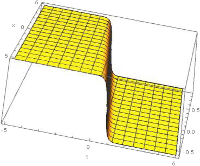
FIGURE 8. Numerical simulation of $u_{\mathrm{2,3}}\left(x,y=1,t\right)$.

Category 2: Taking into account $p=\left[-\mathrm{1,0,1,1}\right]$ and $q=\left[\mathrm{0,0,0,1}\right]$, one achieves that

$\mathrm{\Phi }\left(\xi \right)=-\frac{1}{1+\exp \left(\xi \right)}.$(3.64)

Set 1:

$\omega =\frac{-{\kappa }^2{\delta }_3-\mu {\delta }_4\kappa -{\mu }^2{\delta }_5}{\alpha {\kappa }^3},A_1=\frac{2\left({\kappa }^2{\delta }_3+\mu {\delta }_4\kappa +{\mu }^2{\delta }_5\right)\kappa }{-\beta {\kappa }^3\mu +{\kappa }^2{\delta }_3+\mu {\delta }_4\kappa +{\mu }^2{\delta }_5},B_1=0,$(3.65)

where $\kappa ,\mu ,A_0$ are arbitrary contents.

Substituting the values of the parameters Eq. 3.65 into Eq. 3.64 and Eq. 3.3, one obtains the following kink wave as

$U\left(\xi \right)=\frac{\left(\begin{array}{l}{A}_0\left(-\beta {\kappa }^3\mu +{\kappa }^2{\delta }_3+\mu {\delta }_4\kappa +{\mu }^2{\delta }_5\right)\exp \left(\xi \right)+\left(-\beta \mu A_0-2{\delta }_3\right){\kappa }^3\\ +\left(-2\mu {\delta }_4+A_0{\delta }_3\right){\kappa }^2+\left(-2{\mu }^2{\delta }_5+\mu A_0{\delta }_4\right)\kappa +{\mu }^2{A}_0{\delta }_5\end{array}\right)}{\left(-\beta {\kappa }^3\mu +{\kappa }^2{\delta }_3+\mu {\delta }_4\kappa +{\mu }^2{\delta }_5\right)\left(1+\exp \left(\xi \right)\right)}.$(3.66)

Thereupon, Eq. 1.2 admits the following exact solution

$u_{\mathrm{2,4}}\left(x,y,t\right)=\frac{\left(\begin{array}{l}{A}_0\left(-\beta {\kappa }^3\mu +{\kappa }^2{\delta }_3+\mu {\delta }_4\kappa +{\mu }^2{\delta }_5\right)\exp \left(\xi \right)+\left(-\beta \mu A_0-2{\delta }_3\right){\kappa }^3\\ +\left(-2\mu {\delta }_4+A_0{\delta }_3\right){\kappa }^2+\left(-2{\mu }^2{\delta }_5+\mu A_0{\delta }_4\right)\kappa +{\mu }^2{A}_0{\delta }_5\end{array}\right)}{\left(-\beta {\kappa }^3\mu +{\kappa }^2{\delta }_3+\mu {\delta }_4\kappa +{\mu }^2{\delta }_5\right)\left(1+\exp \left(\xi \right)\right)},$(3.67)

where

$\xi =\kappa x+\mu y+\frac{\left(-{\kappa }^2{\delta }_3-\mu {\delta }_4\kappa -{\mu }^2{\delta }_5\right)}{\alpha {\kappa }^3}t.$(3.68)

Numerical simulation corresponding to the solution $u_{\mathrm{2,4}}\left(x,y=1,t\right)$ while taking $\kappa =0.3,\mu =0.2,\alpha =0.9,\beta =0.8,{\delta }_1=0.5,{\delta }_2=0.3,{\delta }_3=0.2,{\delta }_4=0.5,{\delta }_5=0.8,A_0=0.1$, which is an anti-kink type solution, is presented in Figure 9.

FIGURE 9

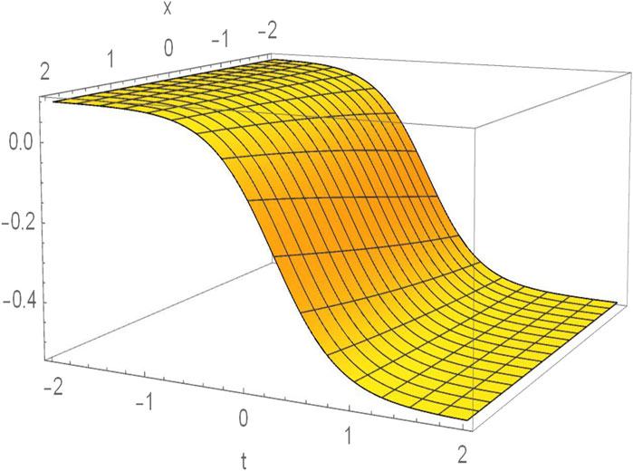
FIGURE 9. Numerical simulation of $u_{\mathrm{2,4}}\left(x,y=1,t\right)$.

Category 3: Taking into account $p=\left[-3,-\mathrm{1,1,1}\right]$ and $q=\left[1,-\mathrm{1,1},-1\right]$, one achieves that

$\mathrm{\Phi }\left(\xi \right)=\frac{-\sinh \left(\xi \right)-2\cosh \left(\xi \right)}{\cosh \left(\xi \right)}.$(3.69)

Set 1:

$\omega =\frac{-{\kappa }^2{\delta }_3-\mu {\delta }_4\kappa -{\mu }^2{\delta }_5}{4\alpha {\kappa }^3},A_1=0,B_1=\frac{6\left({\kappa }^2{\delta }_3+\mu {\delta }_4\kappa +{\mu }^2{\delta }_5\right)\kappa }{-4\beta {\kappa }^3\mu +{\kappa }^2{\delta }_3+\mu {\delta }_4\kappa +{\mu }^2{\delta }_5},$(3.70)

where $\kappa ,\mu ,A_0$ are arbitrary contents.

Substituting the values of the parameters Eq. 3.70 into Eq. 3.69 and Eq. 3.3, one obtains the following wave solution as

$U\left(\xi \right)=\frac{\left(\begin{array}{l}\left(\begin{array}{l}\left(-8\beta \mu A_0-6{\delta }_3\right){\kappa }^3+\left(-6\mu {\delta }_4+2A_0{\delta }_3\right){\kappa }^2\\ +\left(-6{\mu }^2{\delta }_5+2\mu A_0{\delta }_4\right)\kappa +2{\mu }^2{A}_0{\delta }_5\end{array}\right)\cosh \left(\xi \right)\\ +A_0\left(-4\beta {\kappa }^3\mu +{\kappa }^2{\delta }_3+\mu {\delta }_4\kappa +{\mu }^2{\delta }_5\right)\sinh \left(\xi \right)\end{array}\right)}{\left(-4\beta {\kappa }^3\mu +{\kappa }^2{\delta }_3+\mu {\delta }_4\kappa +{\mu }^2{\delta }_5\right)\left(\sinh \left(\xi \right)+2\cosh \left(\xi \right)\right)}.$(3.71)

Thereupon, Eq. 1.2 admits the following exact solution

$u_{\mathrm{2,5}}\left(x,y,t\right)=\frac{\left(\begin{array}{l}\left(\begin{array}{l}\left(-8\beta \mu A_0-6{\delta }_3\right){\kappa }^3+\left(-6\mu {\delta }_4+2A_0{\delta }_3\right){\kappa }^2\\ +\left(-6{\mu }^2{\delta }_5+2\mu A_0{\delta }_4\right)\kappa +2{\mu }^2{A}_0{\delta }_5\end{array}\right)\cosh \left(\xi \right)\\ +A_0\left(-4\beta {\kappa }^3\mu +{\kappa }^2{\delta }_3+\mu {\delta }_4\kappa +{\mu }^2{\delta }_5\right)\sinh \left(\xi \right)\end{array}\right)}{\left(-4\beta {\kappa }^3\mu +{\kappa }^2{\delta }_3+\mu {\delta }_4\kappa +{\mu }^2{\delta }_5\right)\left(\sinh \left(\xi \right)+2\cosh \left(\xi \right)\right)},$(3.72)

where

$\xi =\kappa x+\mu y+\frac{\left(-{\kappa }^2{\delta }_2-\mu {\delta }_4\kappa -{\mu }^2{\delta }_5\right)}{4\alpha {\kappa }^3}t.$(3.73)

Category 4: Taking into account $p=\left[2-i,-2-i,-\mathrm{1,1}\right]$ and $q=\left[i,-i,i,-i\right]$, one achieves that

$\mathrm{\Phi }\left(\xi \right)=\frac{\cos \left(\xi \right)-2\sin \left(\xi \right)}{\sin \left(\xi \right)}.$(3.74)

Set 1:

$\begin{array}{l}\kappa =\kappa ,\mu =\mu ,\omega =\frac{{\kappa }^2{\delta }_3+\mu {\delta }_4\kappa +{\mu }^2{\delta }_5}{4\alpha {\kappa }^3},A_0=A_0,\\ A_1=0,B_1=-\frac{10\left({\kappa }^2{\delta }_3+\mu {\delta }_4\kappa +{\mu }^2{\delta }_5\right)\kappa }{4\beta {\kappa }^3\mu +{\kappa }^2{\delta }_3+\mu {\delta }_4\kappa +{\mu }^2{\delta }_5}.\end{array}$(3.75)

Substituting the values of the parameters Eq. 3.75 into Eq. 3.74 and Eq. 3.3, one obtains the following periodic wave as

$U\left(\xi \right)=\frac{\left(\begin{array}{l}\left(\begin{array}{l}\left(-8\beta \mu A_0-10{\delta }_3\right){\kappa }^3+\left(-10\mu {\delta }_4-2A_0{\delta }_3\right){\kappa }^2\\ +\left(-10{\mu }^2{\delta }_5-2\mu A_0{\delta }_4\right)\kappa -2{\mu }^2{A}_0{\delta }_5\end{array}\right)\sin \left(\xi \right)\\ +A_0\left(4\beta {\kappa }^3\mu +{\kappa }^2{\delta }_3+\mu {\delta }_4\kappa +{\mu }^2{\delta }_5\right)\cos \left(\xi \right)\end{array}\right)}{\left(4\beta {\kappa }^3\mu +{\kappa }^2{\delta }_3+\mu {\delta }_4\kappa +{\mu }^2{\delta }_5\right)\left(\cos \left(\xi \right)-2\sin \left(\xi \right)\right)}.$(3.76)

Thereupon, Eq. 1.2 admits the following exact solution

$u_{\mathrm{2,6}}\left(x,y,t\right)=\frac{\left(\begin{array}{l}\left(\begin{array}{l}\left(-8\beta \mu A_0-10{\delta }_3\right){\kappa }^3+\left(-10\mu {\delta }_4-2A_0{\delta }_3\right){\kappa }^2\\ +\left(-10{\mu }^2{\delta }_5-2\mu A_0{\delta }_4\right)\kappa -2{\mu }^2{A}_0{\delta }_5\end{array}\right)\sin \left(\xi \right)\\ +A_0\left(4\beta {\kappa }^3\mu +{\kappa }^2{\delta }_3+\mu {\delta }_4\kappa +{\mu }^2{\delta }_5\right)\cos \left(\xi \right)\end{array}\right)}{\left(4\beta {\kappa }^3\mu +{\kappa }^2{\delta }_3+\mu {\delta }_4\kappa +{\mu }^2{\delta }_5\right)\left(\cos \left(\xi \right)-2\sin \left(\xi \right)\right)},$(3.77)

Where

$\xi =\kappa x+\mu y+\frac{\left({\kappa }^2{\delta }_3+\mu {\delta }_4\kappa +{\mu }^2{\delta }_5\right)}{4\alpha {\kappa }^3}t.$(3.78)

Numerical simulation corresponding to the solution $u_{\mathrm{2,6}}\left(x,y=1,t\right)$ while taking $\kappa =0.3,\mu =0.2,\alpha =0.3,\beta =0.3,{\delta }_1=0.5,{\delta }_2=0.3,{\delta }_3=0.2,{\delta }_4=0.5,{\delta }_5=0.8,A_0=0.1$, which is a periodic singular solution, is presented in Figure 10.

FIGURE 10

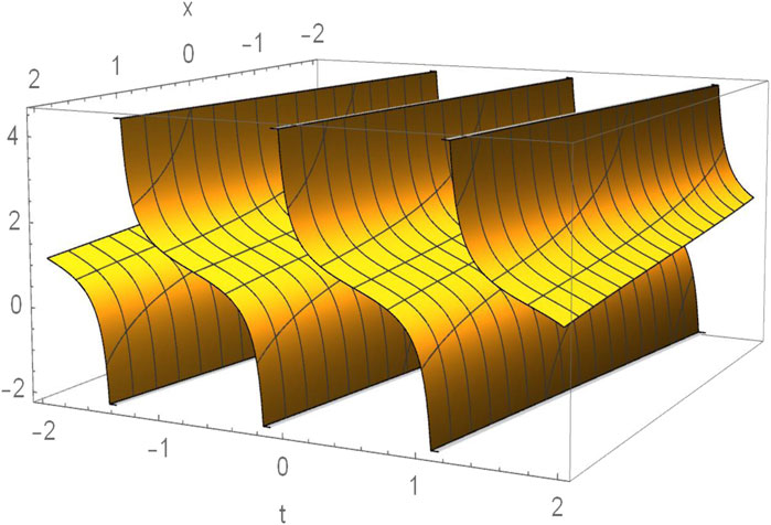
FIGURE 10. Numerical simulation of $u_{\mathrm{2,6}}\left(x,y=1,t\right)$.

So far, via the appropriate choice of free parameters there has six exact solutions are formally presented to Eq. 1.2 which are valuable to demonstrate the propagation of traveling waves.

4 Discussions

i) Based on the balancing equation the pre-constructed solution forms to the examined Eq. 1.1 and Eq. 1.2 are generated as same as Eq. 3.3. Nevertheless, by using the powerful GERFM, seventeen completely different forms of seed solutions can be constructed with distinct physical structures according to their respective dispersion, dissipation and non-linear terms to further demonstrate the significant properties of traveling wave.

ii) It is clear to see that wave amplitude of all extract solutions is directly influenced by wave number $\kappa$ of x direction. Moreover, the wave speed is determined by the coefficients of dissipative terms, u_xx, u_xy, and u_yy.

iii) Based on the crucial idea of GERFM, there has no pre-defined seed solutions to the investigated equations. The seed solutions are derived by the original forms of the examined HSI-like equations [27]. In other words, there has no redundant solutions to our generated results. Although most of the generated solutions are in complex form, 3D plots can show different kinds of wave propagation to help scientists understand the properties of different solutions.

iv) The class of obtained wave solutions is explicitly constructed from the coefficients of the combined non-linear and dissipative terms, including singular, periodic singular, and anti-kink waves. While singular solutions may not be very useful from a physical point of view, they are valuable achievements of GERFM’s approach to the problem from a mathematical point of view.

5 Conclusion

Studying exact solutions of the non-linear problems plays a pivotal role in understanding the non-linear physical phenomena. In this paper, we demonstrate that HSI-like equations still have abundant and interesting solution structures by applying GERFM.

Meanwhile, the traveling singular waves, periodic singular waves and anti-kink waves are presented in Figures through mathematical software Maple. The important properties of traveling waves are elaborated, in which the amplitude is affected by the wave number, and the wave speed is determined by the value of the coefficient of dissipation terms.

To summarize, under specified constraints, eleven exact solutions to Eq. 1.1 and six ones to Eq. 1.2 are formally presented. The singular solutions may be less useful from a physical point of view, but from a mathematical point of view, they are valuable achievements for GERFM to handle high-order and high-dimensional non-linear equations. According to the extracted results, the diversity of non-linear fluid traveling waves related to the HSI equation is brought to light. The presented GERFM is confirmed as an effective mathematical tool for generating abundant wave solutions.

Data availability statement

The original contributions presented in the study are included in the article/supplementary material, further inquiries can be directed to the corresponding authors.

Author contributions

CK conceived of the presented idea. BG performed the computations. CK encouraged CJ to investigate the findings of this work. CJ contributed to the final version of the manuscript. All authors discussed the results and contributed to the final manuscript.

Funding

This work was supported by National Science and Technology Council, Taiwan, under grant numbers MOST 111-2221-E-013-002.

Conflict of interest

The authors declare that the research was conducted in the absence of any commercial or financial relationships that could be construed as a potential conflict of interest.

Publisher’s note

All claims expressed in this article are solely those of the authors and do not necessarily represent those of their affiliated organizations, or those of the publisher, the editors and the reviewers. Any product that may be evaluated in this article, or claim that may be made by its manufacturer, is not guaranteed or endorsed by the publisher.

References

1. Wazwaz AM. Partial differential equations and solitary waves theory. Springer Science & Business Media (2010).

Google Scholar

2. Osman M. One-soliton shaping and inelastic collision between double solitons in the fifth-order variable-coefficient Sawada–Kotera equation. Nonlinear Dyn (2019) 96(2):1491–6. doi:10.1007/s11071-019-04866-1

CrossRef Full Text | Google Scholar

3. Ma YL, Wazwaz AM, Li BQ. Novel bifurcation solitons for an extended Kadomtsev–Petviashvili equation in fluids. Phys Lett A (2021) 413:127585. doi:10.1016/j.physleta.2021.127585

CrossRef Full Text | Google Scholar

4. Shen Y, Tian B, Zhou TY, Gao XT. Shallow-water-wave studies on a (2+1)-dimensional hirota–satsuma–ito system: X-Type soliton, resonant Y-type soliton and hybrid solutions. Chaos, Solitons & Fractals (2022) 157:111861. doi:10.1016/j.chaos.2022.111861

CrossRef Full Text | Google Scholar

5. Kuo CK, Ma WX. A study on resonant multi-soliton solutions to the (2+1)-dimensional Hirota–Satsuma–Ito equations via the linear superposition principle. Nonlinear Anal (2020) 190:111592. doi:10.1016/j.na.2019.111592

CrossRef Full Text | Google Scholar

6. Ma WX. Interaction solutions to Hirota-Satsuma-Ito equation in (2+1)-dimensions. Front Math China (2019) 14(3):619–29. doi:10.1007/s11464-019-0771-y

CrossRef Full Text | Google Scholar

7. Cheng L, Zhang Y, Ma WX. Wronskian $$\pmb {N}$$-soliton solutions to a generalized KdV equation in ($$\pmb {2+1}$$)-dimensions. Nonlinear Dyn (2022) 111:1701–14. doi:10.1007/s11071-022-07920-7

CrossRef Full Text | Google Scholar

8. Akinyemi L, Senol M, Akpan U, Rezazadeh H. An efficient computational technique for class of generalized Boussinesq shallow-water wave equations. J Ocean Eng Sci (2022 Forthcoming). doi:10.1016/j.joes.2022.04.023

CrossRef Full Text | Google Scholar

9. Kuo CK, Kumar D, Juan CJ. A study of resonance Y-type multi-soliton solutions and soliton molecules for new (2+1)-dimensional nonlinear wave equations. AIMS Math (2022) 7(12):20740–51. doi:10.3934/math.20221136

CrossRef Full Text | Google Scholar

10. Zhu HM, Zhang ZY, Zheng J. The time-fractional (2+1)-dimensional hirota–satsuma–ito equations: Lie symmetries, power series solutions and conservation laws. Commun Nonlinear Sci Numer Simulation (2022) 115:106724. doi:10.1016/j.cnsns.2022.106724

CrossRef Full Text | Google Scholar

11. Long F, Alsallami SA, Rezaei S, Nonlaopon K, Khalil E. New interaction solutions to the (2+1)-dimensional hirota–satsuma–ito equation. Results Phys (2022) 37:105475. doi:10.1016/j.rinp.2022.105475

CrossRef Full Text | Google Scholar

12. Song Y, Wang Z, Ma Y, Yang B. Solitary, kink and periodic wave solutions of the (3+ 1)-dimensional Hirota–Satsuma–Ito-like equation. Results Phys (2022) 42:106013. doi:10.1016/j.rinp.2022.106013

CrossRef Full Text | Google Scholar

13. Alharbi YF, El-Shewy EK, Abdelrahman MA. New and effective solitary applications in Schrödinger equation via Brownian motion process with physical coefficients of fiber optics. AIMS Math (2023) 8(2):4126–40. doi:10.3934/math.2023205

CrossRef Full Text | Google Scholar

14. Abdelwahed HG, El-Shewy E, Alghanim S, Abdelrahman MA. Modulations of some physical parameters in a nonlinear Schrödinger type equation in fiber communications. Results Phys (2022) 38:105548. doi:10.1016/j.rinp.2022.105548

CrossRef Full Text | Google Scholar

15. Alkhidhr HA, Abdelwahed H, Abdelrahman MA, Alghanim S. Some solutions for a stochastic NLSE in the unstable and higher order dispersive environments. Results Phys (2022) 34:105242. doi:10.1016/j.rinp.2022.105242

CrossRef Full Text | Google Scholar

16. He XJ, Lü X, Li MG. Bäcklund transformation, pfaffian, wronskian and grammian solutions to the (3+1)-dimensional generalized kadomtsev–petviashvili equation. Anal Math Phys (2021) 11(1):1–24.

CrossRef Full Text | Google Scholar

17. Chen SJ, Ma WX, Lü X. Bäcklund transformation, exact solutions and interaction behaviour of the (3+1)-dimensional Hirota-Satsuma-Ito-like equation. Commun Nonlinear Sci Numer Simulation (2020) 83:105135. doi:10.1016/j.cnsns.2019.105135

CrossRef Full Text | Google Scholar

18. Kudryashov NA. Seven common errors in finding exact solutions of nonlinear differential equations. Commun Nonlinear Sci Numer Simulation (2009) 14(9-10):3507–29. doi:10.1016/j.cnsns.2009.01.023

CrossRef Full Text | Google Scholar

19. Wu J, Li B. Resonant collisions among localized waves in the (2+1)-dimensional Hirota–Satsuma–Ito equation. Mod Phys Lett B (2022) 36:2250148. doi:10.1142/s0217984922501482

CrossRef Full Text | Google Scholar

20. Ghanbari B, Kuo CK. New exact wave solutions of the variable-coefficient (1+1)-dimensional Benjamin-Bona-Mahony and (2+1)-dimensional asymmetric Nizhnik-Novikov-Veselov equations via the generalized exponential rational function method. The Eur Phys J Plus (2019) 134(7):334–13. doi:10.1140/epjp/i2019-12632-0

CrossRef Full Text | Google Scholar

21. Ghanbari B, Osman M, Baleanu D. Generalized exponential rational function method for extended Zakharov–Kuzetsov equation with conformable derivative. Mod Phys Lett A (2019) 34(20):1950155. doi:10.1142/s0217732319501554

CrossRef Full Text | Google Scholar

22. Ghanbari B, Yusuf A, Inc M, Baleanu D. The new exact solitary wave solutions and stability analysis for the (2+1)-dimensional Zakharov–Kuznetsov equation. Adv difference equations (2019) 1 1–15. doi:10.1186/s13662-019-1964-0

CrossRef Full Text | Google Scholar

23. Cevikel AC, Bekir A, Abu Arqub O, Abukhaled M. Solitary wave solutions of Fitzhugh–Nagumo-type equations with conformable derivatives. Front Phys (2022) 1064. doi:10.3389/fphy.2022.1028668

CrossRef Full Text | Google Scholar

24. Wu YH, Liu C, Yang ZY, Yang WL. Non-degenerate rogue waves and multiple transitions in systems of three-wave resonant interaction. Front Phys (2022) 1083. doi:10.3389/fphy.2022.1043053

CrossRef Full Text | Google Scholar

25. Akinyemi L, Veeresha P, Senol M, Rezazadeh H. An efficient technique for generalized conformable Pochhammer–Chree models of longitudinal wave propagation of elastic rod. Indian J Phys (2022) 1-10:4209–18. doi:10.1007/s12648-022-02324-0

CrossRef Full Text | Google Scholar

26. Almutairi A, El-Shewy E, Amin AH, Abdelrahman MA. New solitary electrostatic structures for Zakharov model in subsonic limit for solar-wind. Results Phys (2022) 37:105521. doi:10.1016/j.rinp.2022.105521

CrossRef Full Text | Google Scholar

27. Günay B, Kuo CK. On determining some exact wave solutions to the Nizhnik–Novikov–Veselov system via a rebuts technique. Results Phys (2021) 26:104359. doi:10.1016/j.rinp.2021.104359

CrossRef Full Text | Google Scholar

28. Wang B, Ma Z, Liu X. Dynamics of nonlinear wave and interaction phenomenon in the (3+13+1)-dimensional Hirota–Satsuma–Ito-like equation. The Eur Phys J D (2022) 76(9):1–15. doi:10.1140/epjd/s10053-022-00493-5

CrossRef Full Text | Google Scholar

29. Wan Ali KK, Yokus A, Seadawy AR, Yilmazer R. The ion sound and Langmuir waves dynamical system via computational modified generalized exponential rational function. Chaos, Solitons Fractals (2022) 161:112381. doi:10.1016/j.chaos.2022.112381

CrossRef Full Text | Google Scholar

30. Jannat N, Kaplan M, Raza N. Abundant soliton-type solutions to the new generalized KdV equation via auto-Bäcklund transformations and extended transformed rational function technique. Opt Quan Elect (2022) 54(8):466–15. doi:10.1007/s11082-022-03862-x

CrossRef Full Text | Google Scholar

31. Kumar S, Kumar D. Analytical soliton solutions to the generalized (3+ 1)-dimensional shallow water wave equation. Mod Phys Lett B (2022) 36(02):2150540. doi:10.1142/s0217984921505400

CrossRef Full Text | Google Scholar

32. Ma WX. A search for lump solutions to a combined fourth-order nonlinear PDE in (2+1)-dimensions. J Appl Anal Comput (2019) 9(4):1319–32. doi:10.11948/2156-907x.20180227

CrossRef Full Text | Google Scholar

33. Cheng L, Ma WX. Framework of extended BKP equations possessing N-wave solutions in (2+1)-dimensions. Math Methods Appl Sci (2022) 45(2):749–60. doi:10.1002/mma.7809

CrossRef Full Text | Google Scholar

34. Zhang Y, Ma WX, Yang JY. A study on lump solutions to a (2+1)-dimensional completely generalized Hirota-Satsuma-Ito equation. Discrete & Continuous Dynamical Systems-S (2020) 13(10):2941. doi:10.3934/dcdss.2020167

CrossRef Full Text | Google Scholar