Energy spectra of buoyancy-driven bubbly flow in a vertical Hele-Shaw cell

We present direct numerical simulations (DNS) study of confined buoyancy-driven bubbly flows in a Hele-Shaw setup. We investigate the spectral properties of the flow and make comparisons with experiments. The energy spectrum obtained from the gap-averaged velocity field shows E(k) ∼ k for k < k_d, E(k) ∼ k⁻⁵ for k > k_d, and an intermediate scaling range with E(k) ∼ k⁻³ around k ∼ k_d. We perform an energy budget analysis to understand the dominant balances and explain the observed scaling behavior. For k < k_d, energy injection balances dissipation due to drag, whereas for k > k_d, the net injection balances net dissipation. We also show that the Navier-Stokes equation with a linear drag can be used to approximate large scale flow properties of bubbly Hele-Shaw flow.

1 Introduction

Flows generated by dilute bubble suspensions (bubbly flows) are relevant in many natural and industrial processes [1]. As the bubbles rise due to buoyancy and stir the fluid, they generate complex spatiotemporal flow structures “pseudo-turbulence” [2–6]. The underlying physical mechanisms responsible for the flow are the interaction between wakes caused by individual bubbles and the interaction of bubbles with the flow generated by their neighbors [3,5].

Early experiments characterized pseudo-turbulence in bubbly flows at a low-volume fraction by measuring the energy spectrum E(k) ∼ k⁻³ (where k is the wave number). They argued that the power-law scaling appears due to a balance of energy production with viscous dissipation [2]. Subsequent experimental studies have verified the power-law scaling in the energy spectrum [5,7–9].

Only recent numerical studies have started investigating pseudo-turbulence at experimentally relevant parameter ranges [6,10,11]. A scale-by-scale energy budget analysis has unraveled the details of the energy transfer mechanism. Buoyancy injects energy at scales comparable to the bubble diameter; it is then transferred to smaller scales by non-linear fluxes due to surface tension and kinetic energy, where it gets dissipated by viscosity. Quite remarkably, these studies also reveal that the statistics of the velocity fluctuations do not depend either on the viscosity or density contrast [6,11,12].

How does the physics of bubbly flows altered in the presence of confinement? Earlier studies have investigated this question in a Hele-Shaw setup with bubbles whose unconfined diameter is larger than the confinement width [13–15]. Numerical simulations and experiments [1,16–18] on an isolated rising bubble show that, compared to an unconfined bubble, the wake flow of the confined bubble is severely attenuated. Nevertheless, the experiments on bubbly flows in the Hele-Shaw setup still observe the power-law scaling of pseudo-turbulence between scales comparable to the bubble diameter and twenty times the bubble diameter.

In this paper, we perform a numerical investigation of buoyancy-driven bubbly flow in a Hele-Shaw setup. To make a comparison with experiments, we choose moderate volume fractions ϕ = 5–10%. We investigate the energy spectrum of the gap-averaged velocity field and, consistent with experiments, observe an interediate power-law scaling in the energy spectrum E(k) ∼ k⁻³. Using a scale-by-scale energy budget analysis, we show that confinement dramatically alters the energy budget compared to the unbounded bubbly flows. The viscous drag due to the confining walls balances energy injected by buoyancy at large scales. Non-linear transfer mechanisms due to surface tension and kinetic energy are negligible. Finally, we show that two-dimensional Navier-Stokes equations with an added drag term can be used as a model to study large scale flow properties.

The rest of the paper is organised as follows. In Section 2, we discuss the governing equations and the details of the numerical method used. In Section 3, we present results for bubbly flows in the Hele-Shaw setup and study the energy budget. We then show that the two-dimensional Navier-Stokes equations with a linear drag is a good model to study large scale properties of bubbly flows under confinement. Finally, in Section 4, we present our conclusion.

2 Equations and numerical methods

We study the dynamics of bubbly flows in a vertical Hele-Shaw cell (see Figure 1) by solving the Navier-Stokes equations with surface tension force acting at the interface,

$\begin{array}{cc}\hfill {\partial }_{t}C+\mathbf{U}\cdot {\nabla }^{*}C& =0,\hspace{1em}{\nabla }^{*}\cdot \mathbf{U}=0,\mathrm{a}\mathrm{n}\mathrm{d}\hfill \\ \hfill \varrho \left(C\right)\left({\partial }_t+\mathbf{U}\cdot {\nabla }^{*}\right)\mathbf{U}& ={\nabla }^{*}\cdot \left[\mu \left(C\right)\left({\nabla }^{*}\mathbf{U}+{\nabla }^{*}{\mathbf{U}}^T\right)\right]-{\nabla }^{*}P+{\mathbf{F}}^g+{\mathbf{F}}^{\sigma }\hfill \end{array}.(1)$

Here, ∇* ≡ (∂_x, ∂_y, ∂_z), C is an indicator function whose value is 0 inside the bubble phase and 1 in the fluid phase, ${\mathbf{F}}^g\equiv [{\rho }_a-\varrho (C)]g{\widehat{\mathbf{e}}}_z$ is the buoyancy force, ρ_a = [∫ϱdx]/(L²H) is the average density, U = (U_x, U_y, U_z) is the hydrodynamic velocity, P is the pressure, the local density ϱ(C) ≡ ρ₁C + ρ₂(1 − C), the local viscosity μ(C) ≡ μ₁C + μ₂(1 − C), ρ₂ (ρ₁) is the bubble (fluid) density, μ₂ (μ₁) is the bubble (fluid) viscosity, and F^σ ≡ σκ∇^⋆C is the surface tension force at the interface [19] with σ as the coefficient of surface tension and κ the interface curvature. The bubble volume fraction ϕ ≡ [∫(1 − C)dx]/(L²H), where L is the length along the x − and z − directions, and H is the gap width between the two parallel plates of the Hele-Shaw cell. In what follows, ρ₁ (μ₁) denotes the density (viscosity) of the liquid phase, and ρ₂ (μ₂) denotes the density (viscosity) of the bubble phase.

FIGURE 1

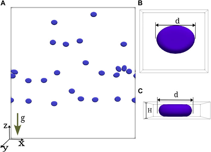
FIGURE 1. (A) Representative plot showing bubbles of diameter d in a Hele-Shaw setup. The length along x −and z −directions is L, and the gap width in y −direction is H; (B) Top view of a bubble (zoomed view); (C) Front view of the bubble (zoomed view).

The non-dimensional numbers that characterize the flow are the Galilei number $\text{Ga}\equiv \sqrt{{\rho }_1\delta \rho gd}d/{\mu }_1$¹, the Bond number Bo ≡ δρgd²/σ, and the Atwood number At ≡ δρ/(ρ₁ + ρ₂) with δρ = (ρ₁ − ρ₂). For brevity, in the following sections, we will refer to (1) as NSHS.

2.1 Gap width averaged equations

Experiments often use gap width averaged velocities to study statistical properties of the flow. Following the procedure outlined in [20,21] and assuming density ϱ to be constant along wall-normal direction, and starting from the NSHS equations, we get the following equations for the gap averaged indicator function c and horizontal components of the velocity²:

$\begin{array}{cc}\hfill \left({\partial }_t+\mathbf{u}\cdot \nabla \right)c& =0,\hspace{1em}\nabla \cdot \mathbf{u}=0,\mathrm{a}\mathrm{n}\mathrm{d}\hfill \\ \hfill \rho \left({\partial }_t+\mathbf{u}\cdot \nabla \right)\mathbf{u}& =-\nabla \cdot \rho \overline{{\mathbf{U}}^{\prime }{\mathbf{U}}^{\prime }}+\nabla \cdot \left(2\bar{\mu }\mathsf{S}\right)+{\bar{\mathbf{F}}}^d-\nabla \bar{P}+{\bar{\mathbf{F}}}^g+{\bar{\mathbf{F}}}^{\sigma }.\hfill \end{array}(2)$

Here, $\overline{(.)}\equiv (1/H){\int }_0^H(.)dy$ denotes gap averaging, ∇ ≡ (∂_x, ∂_z), u ≡ (u_x(x, z), u_z(x, z)) is the gap averaged velocity field with $u_x={\bar{U}}_x$ and $u_z={\bar{U}}_z$, U′(x) = (U_x − u_x, U_z − u_z) are the three-dimensional residual velocity fluctuations, $\bar{P}(x,z)$ is the gap-averaged pressure field, $\mathsf{S}=\nabla \mathbf{u}+\nabla {\mathbf{u}}^T$ is the gap averaged strain-rate tensor, $\rho \equiv \bar{\varrho }$ is the gap averaged density field, ${\bar{\mathbf{F}}}^g=[{\rho }_a-\rho ]g\widehat{z}$ is the buoyancy force, and ${\bar{\mathbf{F}}}^{\sigma }$ is the surface tension force. The viscous dissipation contributes in two parts: (a) small-scale dissipation $\nabla \cdot \left(2\bar{\mu }\mathsf{S}\right)$, and (b) viscous drag due to walls ${\bar{\mathbf{F}}}^d={[\mu (\nabla \mathbf{U}+\nabla {\mathbf{U}}^T)\cdot \widehat{y}]}_0^H$. Previous studies [13,17,18] have argued that the gap-averaged fields appropriately describe the dynamics of bubbly Hele-Shaw flows provided H/d ≤ 1/2. In particular, they model the dynamics of an isolated bubble using two-dimensional Navier-Stokes equations with a linear drag which has similar structure to (2). We will revisit this point later in Section 3.3.

2.2 Numerical method

We use a second-order finite-volume solver PARIS [22] to simulate NSHS (1). For bubble tracking and updating the indicator function PARIS employs a front-tracking method, and the time marching is performed using the first order Euler method.

2.3 Initial conditions and parameters

We consider a cuboid of breadth L_y = H, and with equal length and height (L_x = L_z = L) [see Figure 1]. The simulation domain (L_x, L_y, L_z) is discretized with (N_x, N_y, N_z) equispaced collocation points. We use periodic boundary conditions in the x and z directions, and impose no-slip velocity boundary U = 0 at the walls (y = 0 and y = H) [23]. We place N_b bubbles in random positions and initialize each one as an ellipsoid of volume V = 4.73 × 10³ (mono-disperse suspension). The front tracking module of the PARIS solver [22] employs a symmetry boundary condition for the surface tension force at the walls such that the net force at the wall would be tangent to the wall. This ensures a thin layer of fluid (approximately O(0.13)δy, where δy = H/N_y) between the bubble and the wall. Our grid resolution is comparable (or higher) to a previous numerical study on Hele-Shaw with bubbles [23]. The bubbles are allowed to relax in the absence of gravity until they achieve the equilibrium pan-cake-like configuration [23] with diameter d = 2H.

In Table 1 we summarize the parameters used in our simulations. We choose parameters such that the dimensionless numbers (Ga, Bo, H/d, and ϕ) are comparable to experiments [15,17,18]. We simulate low At = 0.08 and high At = 0.9, and verify that the spectral properties are insensitive to density contrast [6,11,12].

TABLE 1

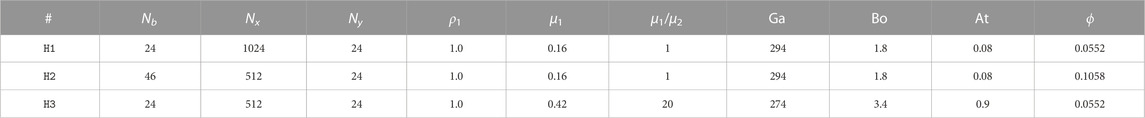
TABLE 1. Parameters used in our simulations. We fix L =512, H = 12, N_x = N_z, and d =24 for all the runs.

3 Results

In this section, we present the results of our numerical investigations. We obtain the density ϱ and the velocity U fields by performing the DNS of NSHS Eq. 1, and from them, we get the corresponding gap averaged fields. We monitor the time evolution of the gap averaged energy and investigate the flow properties in a statistically steady state. The plot in Figure 2 shows a typical snapshot of the bubble configuration along with the flow streamlines in the steady-state. Similar to the experiments [15], we observe that the flow disturbances are mostly localized in the bubble vicinity. Furthermore, the horizontal alignment of bubbles is also observed in experiments [15] as well as numerical simulation of stratified bubbly flows in a Hele-Shaw setup [23]. As is conventional in the experiments [14,15], we investigate the spectral properties of the gap-averaged velocity field (2).

FIGURE 2

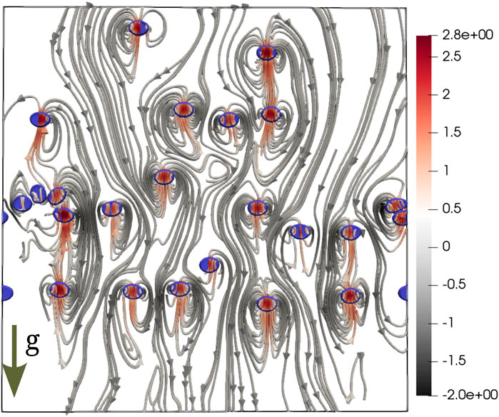
FIGURE 2. Instantaneous bubble configuration superimposed with flow streamlines in the steady-state (run $\mathtt{H}\mathtt{1}$). The streamlines are colored according to the z-component of the velocity.

3.1 Time evolution

From (2), we obtain the following balance equation for the gap-averaged kinetic energy E

${\partial }_t{\displaystyle \underset{E}{{\displaystyle \underbrace{⟨\frac{\rho {\mathbf{u}}^2}{2}⟩}}}}=-{\displaystyle \underset{{ϵ}_{\mu }}{{\displaystyle \underbrace{2⟨\bar{\mu }\mathsf{S}:\mathsf{S}⟩}}}}+{\displaystyle \underset{{ϵ}_{\mathit{inj}}}{{\displaystyle \underbrace{⟨\left[{\rho }_a-\rho \right]u_{z}g⟩}}}}+{\displaystyle \underset{{ϵ}_{\sigma }}{{\displaystyle \underbrace{⟨{\bar{\mathbf{F}}}^{\sigma }\cdot \mathbf{u}⟩}}}}+{\displaystyle \underset{{ϵ}_d}{{\displaystyle \underbrace{⟨{\bar{\mathbf{F}}}^d\cdot \mathbf{u}⟩}}}},(3)$

where ϵ_μ is the gap-averaged viscous energy dissipation, ϵ_d is the dissipation due to drag, ϵ_inj is the gap-averaged energy injected due to buoyancy, ϵ_σ is the contribution due to the surface tension, and the angular brackets denote spatial averaging.

In Figure 3, we plot the time-evolution of the kinetic energy E and observe that a statistically steady state is achieved for t > 0.8τ_s. Furthermore, in Table 2 we show that the energy injected by buoyancy is primarily balanced by the dissipation due to drag in the steady state (∂_tE ≈ 0).

FIGURE 3

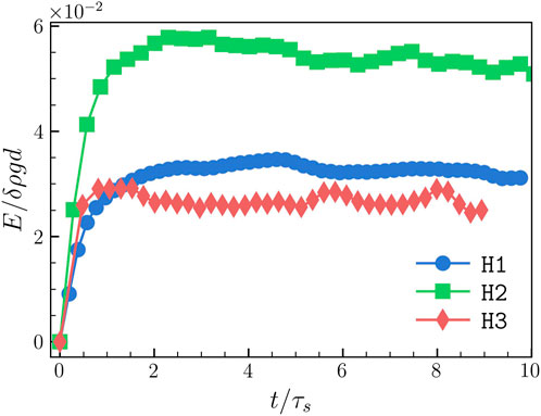
FIGURE 3. Time evolution of the kinetic energy E. A steady-state is attained for t ≥0.8τ_s, where ${\tau }_s=L/\sqrt{gd}$.

TABLE 2

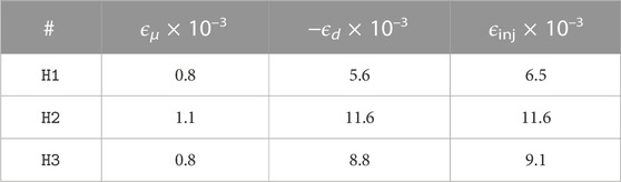
TABLE 2. Time-averaged values of the energy injection ϵ_inj, viscous dissipation ϵ_μ, and dissipation due to drag ϵ_d in the statistically steady state.

3.2 Energy spectra and scale-by-scale energy budget

The energy spectrum and co-spectra for the gap-averaged velocity field are defined as:

$\begin{array}{ll}\hfill E\left(k\right)& \equiv \sum _{k-1/2<m<k+1/2}|\widehat{\mathbf{u}}\left(\mathbf{m}\right){|}^2,\hfill \\ \hfill E^{\rho u}\left(k\right)& \equiv \sum _{k-1/2<m<k+1/2}\mathfrak{R}\left[\widehat{\left(\rho \mathbf{u}\right)}\left(-\mathbf{m}\right)\widehat{\mathbf{u}}\left(\mathbf{m}\right)\right].\hfill \end{array}$

Here, $\widehat{(\cdot )}$ denotes the Fourier transformed fields.

In Figure 4, we plot the energy spectra E(k) and cospectra E^ρu(k) for our simulations $\mathtt{H}1-H3$³. From the plots, we can identify different scaling regimes: (a) For k ≪ k_d we observe E(k) ∼ k, where k_d is the wavenumber corresponding to the bubble diameter; (b) Around k ∼ k_d, we find a short E(k) ∼ k⁻³ scaling regime followed by a steeper decay of the spectrum E(k) ∼ k⁻⁵.

FIGURE 4

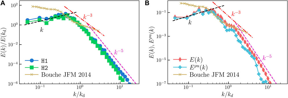
FIGURE 4. (A) Log-log of the energy spectra [E(k) versus k] for low At runs $\mathtt{H}\mathtt{1}$ and $\mathtt{H}\mathtt{2}$. (B) Log-log plot of the energy spectra (E(k)) and cospectra (E^ρu(k)) for high At =0.9 run $\mathtt{H}3$ (Ga =274, ϕ =0.05). We overlay the data extracted from Bouche et al. [15] in both the plots for comparison. The experimental data is scaled vertically for clarity. The data is extracted using the Enguage digitizer [25].

The k⁻³ scaling range observed in our simulaiton is consistent with earlier experiments that also observe an intermediate k⁻³ scaling subrange for 0.2⪅k/k_d⪅1 [15]. We verify this by overlaying the energy spectrum obtained in [15] over our data in Figure 4.

Risso [24] argues that the k⁻³ scaling could be modelled as a signal consisting of a sum of localized random bursts. Although this explanation is consistent with Figure 2, it does not highlight the underlying mechanisms that generate the observed scaling. Lance and Bataille [2] take an alternate viewpoint and argue that the balance of energy production and viscous dissipation leads to the k⁻³ scaling.

The scaling of the energy spectrum we observe differs from earlier studies on two-dimensional unbounded flows [10,12] at comparable Ga. They find an inverse energy cascade with E(k) ∼ k^−5/3 for k < k_d and a E(k) ∼ k⁻³ scaling for k > k_d due to the balance of energy injected by surface tension with viscous dissipation.

In what follows, we present an energy budget analysis to explain the observed scaling of the energy spectrum.

3.2.1 Energy budget

Since the scaling behaviour observed in our simulations $\mathtt{H}1-H3$ is identical, we perform the energy budget analysis using our highest horizontal grid-resolution simulation $\mathtt{H}\mathtt{1}$. Ignoring inertia and assuming a statistically steady state, from (2) we get the following energy budget equation [26,27]:

$\mathcal{F}\left(k\right)+T^{\sigma }\left(k\right)=\underset{D\left(k\right)}{{\displaystyle \underbrace{\nu k^{2}E\left(k\right)}}}+\mathcal{D}\left(k\right),(4)$

where D(k) is the viscous dissipation, $T^{\sigma }(k)={\sum }^{\prime }\mathfrak{R}[{\widehat{\mathbf{F}}}^{\sigma }(\mathbf{m})\cdot \widehat{\mathbf{u}}(-\mathbf{m})]$ is the non-linear transfer due to surface tension, $\mathcal{D}(k)=-{\sum }^{\prime }\mathfrak{R}[{\widehat{\mathbf{F}}}^d(\mathbf{m})\cdot \widehat{\mathbf{u}}(-\mathbf{m})]$ is the viscous dissipation due to drag, $\mathcal{D}(k)={\sum }^{\prime }\mathfrak{R}[{\widehat{F}}^g(\mathbf{m}){\widehat{u}}_z(-\mathbf{m})]$ is the energy injection due to buoyancy. Here, ${\sum }^{\prime }\equiv {\sum }_{|\mathbf{m}|<k-1/2}^{k+1/2}$ indicates summation over all wave-numbers in a circular shell around wavenumber k.

The plot in Figure 5A shows the different contributions to the budget. Clearly for k < k_d, the energy injected by buoyancy is balanced by the drag $(F^g(k)\sim \mathcal{D}(k))$ and other contributions are subdominant. This justifies our assumption of ignoring the inertial terms. In Figure 5B, we show that a linear drag approximation F^d(k) ∼ αE(k) (with α = 0.04) is in excellent agreement with $\mathcal{D}(k)$. Next we approximate the energy injected by buoyancy as $F^g(k)\sim \sqrt{E(k)E_{\rho }(k)}$, where $E_{\rho }(k)={\sum }^{\prime }|\widehat{\rho }(\mathbf{m}){|}^2$. Noting that for k ≪ k_d, i.e., for scales much larger than bubble size, the density field can be approximated by white noise E_ρ(k) ∼ k and by balancing the energy injected by buoyancy with drag, we obtain E(k) ∼ k. This explains the scaling observed in our simulations for k < k_d.

FIGURE 5

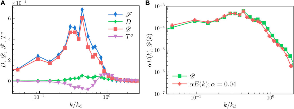
FIGURE 5. (A) Lin-log plot of the different contributions to the spectral energy budget (4) obtained from run $\mathtt{H}\mathtt{1}$. (B) Log-log plot showing comparison of the scaled energy spectrum αE(k) and the dissipation due to drag $\mathcal{D}$(k) for k/k_d <2.

The situation is more complicated for k > k_d. The zoomed-in plot of the energy balance (see Figure 6A) reveals that both buoyancy and the surface tension inject energy that gets dissipated by the viscous forces $(D+\mathcal{D})$, and there is no dominant balance $(\mathcal{D}+T^{\sigma }\sim D+\mathcal{D})$. In Figure 6B, we show that the net dissipation $D+\mathcal{D}\sim kE(k)$. Similarly, the net production $\mathcal{D}+T^{\sigma }\sim k^{-4}$ for k > k_d (see Figure 6C). Therefore, by balancing the net injection with dissipation we get E(k) ∼ k⁻⁵ scaling for k > k_d. Note that the oscillations in T^σ appear with period k_d. Similar oscillations have been also observed in the energy spectrum of confined [23] bubbly flows.

FIGURE 6

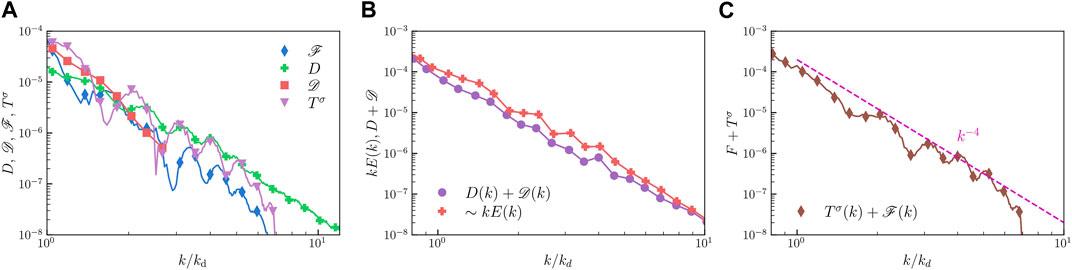
FIGURE 6. (A) Zoomed in plot showing contributions to the spectral energy budget for k > k_d. (B) Log-log plot showing comparison of the scaled dissipation spectrum ∼ kE(K) and the net dissipation $D(k)+\mathcal{D}(k)$ for k > k_d. (C) Log-log plot showing different scaling regimes in the net energy injection $\mathcal{F}(k)+T^{\sigma }(k)$ for k > k_d.

Given the limited cross-over scaling range E(k) ∼ k⁻³ in Figure 4, we are unable to argue about the underlying mechanisms. Thus the plausible explanation for the −3 scaling is the argument by Risso [24] that we have discussed in the previous section.

3.3 Two-dimensional Navier-Stokes equations with a linear drag (NSD)

In this section we investigate whether two-dimensional Navier-Stokes equations with a linear drag coefficient (5) are able to model the confined bubbly flows In the following, we assume all the fields are two-dimensional and for comparison with the gap-averaged quantities, we choose the same symbols.

$\begin{array}{cc}\hfill D_{t}c& =0,\mathrm{a}\mathrm{n}\mathrm{d}\nabla \cdot \mathbf{u}=0,\hfill \\ \hfill \rho \left(c\right)D_t\mathbf{u}& =\nabla \cdot \left[2\mu \left(c\right)\mathsf{S}\right]-\nabla P+{\mathbf{F}}^g+{\mathbf{F}}^{\sigma }-\alpha \mathbf{u}.\hfill \end{array}(5)$

Earlier studies [13,17,18,28] have used NSD Eq. 5 to investigate the dynamics of an isolated bubble in a Hele-Shaw setup with H/d ≤ 0.5 and found the results to be consistent with the experiments. In the following, we use NSD equations to study bubbly flows.

We perform direct numerical simulation of NSD equations on a square domain of area L² and discretize it with 2048² equi-spaced points. The bubbles are initialized as circles of diameter d = 24 and all the parameters of the simulation are identical to our run $\mathtt{H}\mathtt{1}$ and we fix the drag coefficient α = 0.04. Our choice for the value of α is motivated by Figure 5. We use a front-tracking-pseudo-spectral method to evolve (5). For details of the numerical scheme, we refer the reader to Ramadugu et al. [12]. Below we discuss the statistical properties of the flow in the steady state.

In Figure 7A, we plot the bubble configuration and the flow streamlines. Clearly the large scale flow properties resemble those observed for the NSHS simulation. The flow disturbances are localized in the vicinity of the bubbles and we also observe horizontal alignment of bubbles.

FIGURE 7

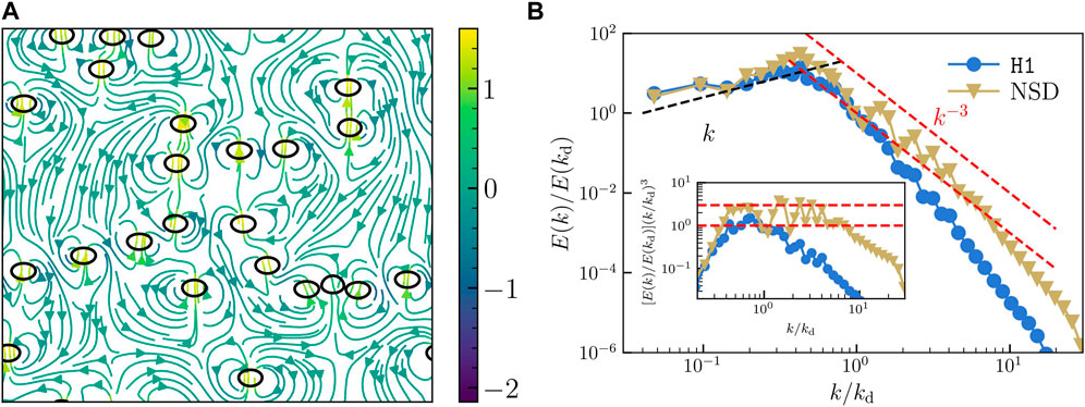
FIGURE 7. (A) Snapshot of the bubble positions overlaid with flow streamlines. (B) Comparison of the gap-averaged energy spectra for our NSHS run $\mathtt{H}\mathtt{1}$ with the energy spectra obtained using simulation of the NSD Eq. 5. (Inset) The compensated spectra k³E(k) is drawn to highlight the −3 scaling range observed for $\mathtt{H}\mathtt{1}$ and NSD simulation.

The plot in Figure 7B shows a comparison of the gap-averaged energy spectrum E(k) obtained from the NSHS equation with that obtained from NSD Eq. 5. We find that the energy spectrum are nearly identical for k < k_d, E(k) ∼ k. However, discrepancies are observed for k > k_d, in contrast to E(k) ∼ k⁻⁵ for the NSHS simulations we find E(k) ∼ k⁻³ for the NSD simulations. As pointed out in earlier section, the oscillation in the energy spectrum appear with a period k_d.

Using (5), and ignoring the inertial contributions, we obtain the following energy balance

$\mathcal{F}\left(k\right)+T^{\sigma }\left(k\right)={\displaystyle \underset{D}{{\displaystyle \underbrace{\nu k^{2}E\left(k\right)}}}}+{\displaystyle \underset{\mathcal{D}}{{\displaystyle \underbrace{\alpha E\left(k\right)}}}}.(6)$

In Figure 8, we plot the contribution of different terms in (6) towards energy balance. For k < k_d, similar to NSHS, we observe that energy injected by buoyancy is balanced by the linear drag. However, a different balance appears for k > k_d. In contrast to NSHS, a dominant balance is observed in the NSD equations. The energy transfer by surface tension to small scales balances viscous dissipation leading to the observed E(k) ∼ k⁻³ scaling in the energy spectrum. Similar small-scale balance has also been reported in earlier two-dimensional unbounded bubbly flow simulations [12]. Therefore, we conclude that although the NSD model captures the large scale dynamics of the Hele-Shaw flow (NSHS), it is unable to correctly capture the small scale physics.

FIGURE 8

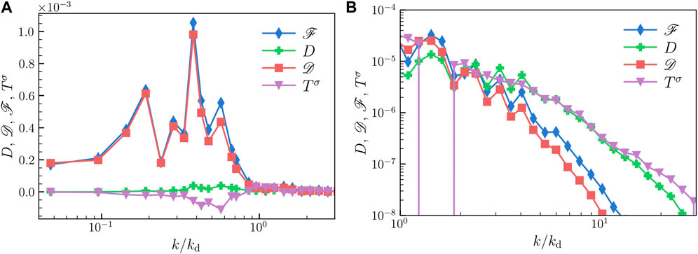
FIGURE 8. Different contributions towards the energy budget for (A) k < k_d and (B) k > k_d obtained from NSD simulation.

4 Conclusion

We have investigated the spectral properties of the two-dimensional bubbly flows under confinement in a Hele-Shaw setup for experimentally relevant Ga and ϕ. The flow visualization in the steady state is similar to earlier experimental observations [15]. The energy spectrum obtained from the gap-averaged velocity field shows E(k) ∼ k for k < k_d and E(k) ∼ k⁻⁵ for k > k_d. We also observe an intermediate scaling range with E(k) ∼ k⁻³ around k ∼ k_d. A scale-by-scale energy budget analysis reveals the dominant balances. For k < k_d, energy injection balances dissipation due to drag, whereas for k > k_d, the net injection balances net dissipation. Finally, we show that the Navier-Stokes equation with a linear drag can be used to approximate large scale flow properties of bubbly Hele-Shaw flow but it fails to correctly capture energy balance at scales smaller than the bubble diameter.

Data availability statement

The raw data supporting the conclusion of this article will be made available by the authors, without undue reservation.

Author contributions

PP contributed to conception and design of the study. RR and VP contributed equally. RR performed initial NSHS and NSD simulations. VP performed NSHS simulations. VP and PP performed the analysis and wrote the manuscript. All authors read, and approved the submitted version.

Funding

We acknowledge support from the Department of Atomic Energy (DAE), India under Project Identification No. RTI 4007, and DST (India) Project Nos. ECR/2018/001135, MTR/2022/000867, and DST/NSM/R&D_HPC_Applications/2021/29.

Conflict of interest

The authors declare that the research was conducted in the absence of any commercial or financial relationships that could be construed as a potential conflict of interest.

Publisher’s note

All claims expressed in this article are solely those of the authors and do not necessarily represent those of their affiliated organizations, or those of the publisher, the editors and the reviewers. Any product that may be evaluated in this article, or claim that may be made by its manufacturer, is not guaranteed or endorsed by the publisher.

Supplementary material

The Supplementary Material for this article can be found online at: https://www.frontiersin.org/articles/10.3389/fphy.2023.1112304/full#supplementary-material

Footnotes

¹Alternatively referred to as the Archimedes number.

²See Supplementary Material for a detailed derivation.

³As the density contrast is negligible for the low At, we do not plot the co-spectra for $\mathtt{H}1,H2$.

References

1. Clift R, Grace JR, Weber ME. Bubbles, drops and particles. New York: Academic Press (1978).

Google Scholar

2. Lance M, Bataille J. Turbulence in the liquid phase of a uniform bubbly air–water flow. J Fluid Mech (1991) 222:95–118. doi:10.1017/s0022112091001015

CrossRef Full Text | Google Scholar

3. Risso F. Agitation, mixing, and transfers induced by bubbles. Annu Rev Fluid Mech (2018) 50:25–48. doi:10.1146/annurev-fluid-122316-045003

CrossRef Full Text | Google Scholar

4. Mudde RF. Gravity-driven bubbly flows. Annu Rev Fluid Mech (2005) 37:393–423. doi:10.1146/annurev.fluid.37.061903.175803

CrossRef Full Text | Google Scholar

5. Mathai V, Lohse D, Sun C. Bubbly and buoyant particle–laden turbulent flows. Annu Rev Condens Matter Phys (2020) 11:529–59. doi:10.1146/annurev-conmatphys-031119-050637

CrossRef Full Text | Google Scholar

6. Pandey V, Ramadugu R, Perlekar P. Liquid velocity fluctuations and energy spectra in three-dimensional buoyancy-driven bubbly flows. J Fluid Mech (2020) 884:R6. doi:10.1017/jfm.2019.991

CrossRef Full Text | Google Scholar

7. Riboux G, Risso F, Legendre D. Experimental characterization of the agitation generated by bubbles rising at high Reynolds number. J Fluid Mech (2010) 643:509–39. doi:10.1017/s0022112009992084

CrossRef Full Text | Google Scholar

8. Prakash VN, Mercado JM, Wijngaarden LV, Mancilla E, Tagawa Y, Lohse D, et al. Energy spectra in turbulent bubbly flows. J Fluid Mech (2016) 791:174–90. doi:10.1017/jfm.2016.49

CrossRef Full Text | Google Scholar

9. Mendez-Diaz S, Serrano-Garcia JC, Zenit R, Hernández-Cordero JA. Power spectral distributions of pseudo-turbulent bubbly flows. Phys Fluids (2013) 25:043303. doi:10.1063/1.4800782

CrossRef Full Text | Google Scholar

10. Innocenti A, Jaccod A, Popinet S, Chibbaro S. Direct numerical simulation of bubble-induced turbulence. J Fluid Mech (2021) 918:A23. doi:10.1017/jfm.2021.288

CrossRef Full Text | Google Scholar

11. Pandey V, Mitra D, Perlekar P. Turbulence modulation in buoyancy-driven bubbly flows. J Fluid Mech (2022) 932:A19. doi:10.1017/jfm.2021.942

CrossRef Full Text | Google Scholar

12. Ramadugu R, Pandey V, Perlekar P. Pseudo-turbulence in two-dimensional buoyancy-driven bubbly flows: A dns study. Eur Phys J E (2020) 43:73–8. doi:10.1140/epje/i2020-11997-0

PubMed Abstract | CrossRef Full Text | Google Scholar

13. Roig V, Roudet M, Risso F, Billet A-M. Dynamics of a high-Reynolds-number bubble rising within a thin gap. J Fluid Mech (2012) 707:444–66. doi:10.1017/jfm.2012.289

CrossRef Full Text | Google Scholar

14. Bouche E, Roig V, Risso F, Billet A. Homogeneous swarm of high-Reynolds-number bubbles rising within a thin gap. Part-1. Bubble dynamics. J Fluid Mech (2012) 704:211–31. doi:10.1017/jfm.2012.233

CrossRef Full Text | Google Scholar

15. Bouche E, Roig V, Risso F, Billet A. Homogeneous swarm of high-Reynolds-number bubbles rising within a thin gap. Part-2. Liquid dynamics. J Fluid Mech (2014) 758:508–21. doi:10.1017/jfm.2014.544

CrossRef Full Text | Google Scholar

16. Kelley E, Wu M. Path instabilities of rising air bubbles in a Hele-Shaw cell. Phys Rev Lett (1997) 79:1265–8. doi:10.1103/physrevlett.79.1265

CrossRef Full Text | Google Scholar

17. Wang X, Klaasen B, Degrève J, Blanpain B, Verhaeghe F. Experimental and numerical study of buoyancy-driven single bubble dynamics in a vertical Hele-Shaw cell. Phys Fluids (2014) 26:123303. doi:10.1063/1.4903488

CrossRef Full Text | Google Scholar

18. Filella A, Patricia E, Roig V. Oscillatory motion and wake of a bubble rising in a thin-gap cell. J Fluid Mech (2015) 778:60–88. doi:10.1017/jfm.2015.355

CrossRef Full Text | Google Scholar

19. Brackbill JU, Kothe DB, Zemach C. A continuum method for modeling surface tension. J Comput Phys (1992) 100:335–54. doi:10.1016/0021-9991(92)90240-y

CrossRef Full Text | Google Scholar

20. Gondret P, Rabaud M. Shear instability of two-fluid parallel flow in a Hele–Shaw cell. Phys Fluids (1997) 9:3267–74. doi:10.1063/1.869441

CrossRef Full Text | Google Scholar

21. Alexakis A, Biferale L. Cascades and transitions in turbulent flows. Phys Rep (2018) 767:1–101. doi:10.1016/j.physrep.2018.08.001

CrossRef Full Text | Google Scholar

22. Aniszewski W, Arrufat T, Crialesi-Esposito M, Dabiri S, Fuster D, Ling Y, et al. Parallel, robust, interface simulator (Paris). Comp Phys Commun (2021) 263:107849. doi:10.1016/j.cpc.2021.107849

CrossRef Full Text | Google Scholar

23. Ganesh M, Kim S, Dabiri S. Induced mixing in stratified fluids by rising bubbles in a thin gap. Phys Rev Fluids (2020) 5:043601. doi:10.1103/physrevfluids.5.043601

CrossRef Full Text | Google Scholar

24. Risso F. Theoretical model for k⁻³ spectra in dispersed multiphase flows. Phys Fluids (2011) 23:011701. doi:10.1063/1.3530438

CrossRef Full Text | Google Scholar

25. Mitchell M, Muftakhidinov B, Tobias W (2023). Engauge digitizer software. markummitchell. Available at: github.io/engauge-digitize

Google Scholar

26. Verma M. Energy transfers in fluid flows. Cambridge University Press (2019).

Google Scholar

27. Pope S. Turbulent flows. Cambridge University Press (2012).

Google Scholar

28. Wang X, Klaasen B, Degrève J, Mahulkar A, Heynderickx G, Reyniers M-F, et al. Volume-of-fluid simulations of bubble dynamics in a vertical Hele-Shaw cell. Phys Fluids (2016) 28:053304. doi:10.1063/1.4948931

CrossRef Full Text | Google Scholar

29. Bretherton F. The motion of long bubbles in tubes. J Fluid Mech (1961) 10:166–88. doi:10.1017/s0022112061000160

CrossRef Full Text | Google Scholar

30. Denkov ND, Tcholakova S, Golemanov K, Subramanian V, Lips A. Foam–wall friction: Effect of air volume fraction for tangentially immobile bubble surface. Colloids Surf A Physicochem Eng Asp (2006) 282-283:329–47. doi:10.1016/j.colsurfa.2006.04.028

CrossRef Full Text | Google Scholar