 Zhaoxuan Zhang1,2
 Hao Liu
- 1School of Physics and Astronomy, Sun Yat-Sen University, Tangjia, Zhuhai, China
- 2School of Physics and Optoelectronics Engineering, Anhui University, Hefei, Anhui, China
- 3Key Laboratory of Particle and Astrophysics, Institute of High Energy Physics (CAS), Beijing, China
- 4CSST Science Center, Zhuhai, China
- 5Peng Cheng Laboratory, Shenzhen, China
Time-ordered data (TOD) from ground-based CMB experiments is usually filtered before map-making to reduce the contamination from ground and atmospheric emissions. However, when the observation region contains strong point sources, the filtering process will cause a considerable leakage around the point sources, which should be eliminated to provide a clean CMB polarization map for scientific purposes. The method we introduce in this work, which we refer to as “template fitting,” is capable of removing these leakage signals in the pixel domain, meeting the requirement of measuring the primordial gravitational waves from CMB-B modes for at least r < 0.005, while also avoiding time-consuming operations on the TOD.
1 Introduction
The cosmic microwave background (CMB) temperature and polarization anisotropies are strong observational evidence of the inflationary expansion history of the Universe. Especially, the detection of B-mode CMB polarization in form of the tensor-to-scalar ratio, r, is crucial for confirming the existence of the gravitational waves in the early Universe, which is a natural consequence of the inflationary potential. Several space and ground-based experiments are devoted to constraining r, including the BICEP series [1], Planck [2], QUIJOTE [3], ACTPol [4], SPTPol [5]. Current observations have already provided limits to r ≲ 0.036–0.1 [6–10], and the forthcoming experiments including POLARBEAR [11], LiteBIRD [12], CMB-S4 [13], the Simons Observatory [14], and AliCPT [15] will devote to reaching a high sensitivity of r ∼ 0.001. This inevitably requires dedicated treatments of all kinds of contamination and systematics. Especially, all available CMB experiments in the next 5–10 years are ground-based, which are ineluctably contaminated by the atmosphere and ground emissions. In order to produce clean sky maps, filtering of modes (including polynominal filtering) in the time ordered data (TOD) is used in many CMB experiments to avoid/alleviate these contaminations, and has become a standard procedure in data processing pipeline of ground-based CMB experiments, such as in the BICEP2/Keck experiment [8], the Simons Observatory [14], and AliCPT [16].
Usually, in a ground-based experiment (e.g., BICEP or AliCPT), the observed TOD is converted to the T, Q, and U maps by the data analysis pipeline that contains data splitting and cutting, pointing and polarization orientation reconstruction (for each detector), time domain filtering, and the final time-to-pixel domain map making. First of all, the TOD are split in units of “halfscan,” and “scanset” (tens of neighbouring halfscans), and bad data are removed at certain thresholds. After that, the pointing trajectory and polarization orientation for each detector are constructed from the encoder data, GPS time, site location as well as the focal plane structure, then the TOD are high-passed to suppress long-distance correlations arising from noise sources or systematic errors. In order to remove the atmospheric radiation present in the data, a polynomial filter (typically of the 3rd order) is applied, and to handle noise associated with the ground coordinate system, such as ground reflections/emissions, templates are constructed and removed for each scanset, which is called a ground subtraction filter. In addition, as a polarization experiment targeting the CMB B-mode, the temperature-polarization leakages need to be removed as much as possible, e.g., by using a de-projection filter on scansets to suppress the leakage due to the beam mismatch of orthogonal polarization detector pairs. It is worth noting that all the filters mentioned above are linear, so it is possible to implement them either as direct time domain operations, or as pixel domain matrix operations, which are completely equivalent. After all these operations, the TOD is weighted by the inverse variance estimated from each scanset, and then projected and co-added on the sky for each map pixel, to produce the final observed map.
Unfortunately, although the TOD filtering can efficiently remove the atmosphere/ground emissions, as well as fixing some other errors, it will also remove part of the CMB signal and cause leakages from point sources to the pixel domain regions around them. Because the latter usually has no preference for the E- and B-modes, when the point source is strong, it can significantly contaminate the weak primordial B-mode signal in a large pixel domain region. For measuring the primordial gravitational waves through the extremely faint B-mode signal, this kind of leakage has to be removed accurately.
In principle, if one knows the sky location of point sources, then it is possible to identify their positions in TOD and cut the corresponding TOD segments to prevent the leakage due to filtered point sources. However, this will cause several problems: 1) Most point sources are not strong enough to be identified from the TOD, because the TOD is much noisier than the final stacked sky map. 2) Removal of the TOD segments containing the point source will compromise the TOD’s integrity, which is disruptive and lead to filtering and mapmaking problems. 3) Typically, operations on TOD are very time-consuming; thus, removal of the point source leakage directly in the TOD is quite expensive. 4) Finally, even if some point sources can be identified through external data, such as radio and optical observations, it is still difficult to subtract them directly from the TOD because their polarization intensities in the CMB bands are usually unknown.
In this work, we introduce a new method to remove the point source leakage due to filtering of the TOD. This method is based on [17] and operates mainly in the pixel domain. The main idea is to construct ideal and realistic templates of the leakages in the pixel domain, and then remove the leakages by linear regression. The advantage of this method is obvious: 1) This method does not cut the TOD, which is friendly to all types of TOD operations. 2) From the test results, this method can successfully remove the point source leakage down to the level satisfying the detection requirement of at least r ≤ 0.005. 3) This method operates mainly in the pixel domain, which is fast and easy to implement.
The structure of this paper is as follows: in Section 2, we introduce our removal of point source leakage method for both single and multiple point sources. We give examples for these two situations and use actual point source data to verify our method in Section 3. Finally, we summarize and conclude in Section 4.
2 Methods
The core concept to alleviate the point source leakages on the final sky map is based on the fact, that all TOD operations and their effects in the pixel domain sky maps are linear. In order to remove the leakages by linear regression, the fundamental operation is to create pixel domain leakage templates. Since the data we obtain from the pipeline is always filtered, two types of templates can be produced: ideal and realistic. The main difference between them is that the ideal template requires complete knowledge of the beam profile, which is usually unavailable1; whereas a realistic template is constructed directly from the product of the pipeline, which is always available. The performance of the ideal template is certainly better, but, as we will mention below, the results of cleaning by the realistic template are also acceptable.
2.1 The ideal template
Construction of the ideal template is straightforward: the filtered sky map D′ produced by the pipeline is
where dp is a single point source (assumed to have Gaussian shape in simulation) and
is a column vector containing the input signals other than the point sources: dc is the CMB signal, df is the foreground, and n is the noise. F is a square matrix representing the linear filtering effect. M is a diagonal matrix for the point source mask, which is 1 for the region around the point source and 0 elsewhere, and I is the identity matrix. Thus, I − M is the non-point source region where the point source leakages need to be studied. For convenience, the filtered result of d is also computed as
note that both d and d′ are without the point source or point source leakages.
It is clear from the descriptions above that the ideal template
which fully contains the point source leakage due to filtering except for an unknown point source amplitude2. If the amplitude of the template can be perfectly determined, then we have
which separates the signal and point source leakages completely. In practice, the amplitude of the template should be determined by linear regression, and the best-fit template is subtracted to remove the point source leakage, leaving a residual that is no more than the chance correlation between
2.2 The realistic template
The ideal template can remove the point source leakages more effectively, but it necessitates precise knowledge of the beam profile, including the asymmetry, which is usually unavailable. Therefore, we go forward with creating a realistic template that can be obtained directly from the sky map produced by the pipeline. The main idea to construct the realistic template is based on three reasonable assumptions:
I The point sources are almost unaffected by the TOD filtering. This is true according to Ghosh et al. [16], which shows the small scale structures are almost unaffected by the TOD filtering.
IIThe point source mask is big enough to include the majority of the point source. According to Li et al. [18]; Salatino et al. [19], the FWHM of AliCPT beam varies from 12′ ∼ 19′, which corresponds to the Gaussian beam width of σ < 10′. Therefore, a mask of r = 40′ region is enough to exclude most point sources, with an exception of only a few extremely bright sources along the Galactic plane, which is usually not used for CMB studies.
III The point source is significantly stronger than the CMB/foreground at the position of itself. Although it is possible to detect point sources that are weaker than the CMB, the leakages produced by these point sources are negligible, thus their leakages don’t need to be taken into account.
With assumption I, it is easy to see that dp ≈ F ⋅dp, and assumption II ensures dp ≈ M ⋅dp, which means dp does not change significantly for left multiplication by either F or M; thus, we have:
substitute the above one into Eq. 4, we get the realistic template
The above equation is crucial: As already mentioned above, it is impossible to acquire the true leakage because dp is unknown3. However, M ⋅F ⋅M ⋅dp is nothing more than the filtered sky map in the point source regions (assume III); thus, we may obtain a reasonable estimate of the true point source leakage by feeding the available term M ⋅F ⋅M ⋅dp into the pipeline instead of dp. Therefore, the concept of Eqs 6, 7 is to compute an available approximation of the unavailable true point source leakage.
2.3 Other procedures
The aforementioned method is firstly tested using a single point source simulation. First, Eq. 1 constructs the filtered sky map, and Eqs 4, 7 provide the ideal and realistic templates
where i is pixel number, n is the total number of pixels, the superscripts Q and U of σ denote the Stokes parameters, the subscript Q or U on the right term stands for the Stokes parameter vector solely considered in this formula, and ξ = 0, 1 for the ideal or realistic templates respectively.
If the point source’s polarization direction is unknown, we construct separately
where the Stokes parameter vector is solely taken into account in the formula by the subscript Q (or U) of the right term.
We also test our method with multiple point sources. The filtered sky map D′ is shown here as follows:
where j is the index of point source, MΣ = ∑jMj is the mask for all point sources4 and Mj is the jth single point source mask, and I − MΣ is the non-point source region to investigate the impact of leakage. Hence the ideal and realistic templates for each point source are:
correspondingly, the fitting parameters kξj (when the polarization direction is known) or
and if the polarization directions are unknown, then the RMS are:
3 Simulations and tests
In the computation that follows, we use the outcome with the local monopoles subtracted from each Stokes parameter in the non-point source region, in order to demonstrate the ability of our method to correct the leakages. We also use the average of 10 different CMB and noise realizations to reduce the accidental fluctuation. We first validate the correction method for r = 0.023, and then further demonstrate the validity of our method with simulations of a much smaller value of r = 0.005. However, we also point out that, because the point sources used in our simulation are significantly stronger than what they could be in reality, r = 0.005 is a very conservative estimation of our method’s capacity.
After determining the fitting parameters by multi-linear regression, we build dB (20 log10P) sky maps of the two templates, their residuals and compute the dB effect as
and when the polarization direction is unknown, the residual is:
where ξ = 0, 1 for the ideal and realistic templates, respectively. Now we introduce a quantity,
where the superscript dB stands for the units of decibels. In general, p stands for the polarization intensity, determined by
here θ is the polarizing angle, which are related to the Stokes parameters Q and U by
hence, Pδ denotes the polarization residual for the ideal or realistic template, and ⟨Pcmb⟩ is the mean value of CMB polarization intensity, about 2.07 μK.
3.1 Single point source
In the case of r = 0.023 and for a single point source, the fitting parameter for the ideal template is very close to 1, whereas the fitting parameter for the realistic template is above 1, because the amplitude of the point source is reduced by the TOD filtering. The residual leakages after correction are 1 to 2 orders of magnitudes less than the point source leakage template.
We select a location at [b, l] = [50°, 190°], assuming that its polarization intensity is equal to 150 μK5. We then smooth this point by 19′ to make a Gaussian point source. We first assume that the polarization direction is already known, where we fix the polarization angle of this point source to be 22.5°, resulting in a Gaussian point source with the Q, U values of approximately 106 μK. For this artificially point source, the fitting parameter with true leakage is close to 1.004 and polarization residual standard deviation is approximately 1.339 × 10⁻³ μK in the pixel domain. The fitting parameter with the realistic template is close to 1.205, and the polarization residual standard deviation is roughly 2.115 × 10⁻³ μK in the pixel domain. Meanwhile, the true leakage and the realistic template have standard deviations of 0.028 μK and 0.024 μK for polarization, respectively. Additionally, after filtering calculation, the standard deviations of the CMB polarization, foreground and noise are 0.334 μK, 0.027 μK, and 0.121 μK, respectively. After using our method to alleviate the impact of point source leakage, the standard deviation of residuals is orders of magnitudes smaller than either the template or the CMB, foreground, noise.
For a single Gaussian point source with a given polarization direction, the polarization dB value of templates, residuals and dB effects, are presented in Figure 1. The leakage of point source has a diffused star-like structure in the observation region, as seen in Figure 1, and the residual has a similar shape but is much weaker. Additionally, the dB effect shows that the residual power spectrum is expected to be 3–6 orders of magnitudes lower than the CMB spectrum, and the ideal dB effect is slightly better than the realistic dB effect, which is consistent with expectation.
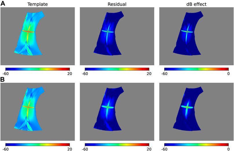
FIGURE 1. Comparison of results in units of decibels (dB) for r = 0.023, obtained using the ideal template (A) and the realistic template (B), for the case of a single point source with a given polarization direction, where the polarization values of the templates (left), the residuals (middle) from Eq. 14 and the dB effects (right) as defined in Eq. 16 are shown, respectively.
We then compute the angular power spectrum of CMB, residual, and true leakage to demonstrate the effect of correction in the harmonic domain, as shown in Figure 2. We select ℓ in the range of 20–600, and the residual spectra (i.e., the power spectra of δξ calculated by Eq. 14, where the filtered CMB signal has been subtracted out) are 2 or 3 orders of magnitudes lower than that of the templates. In addition, there are some fluctuations of the BB power spectrum for CMB in small multipole ℓ as we only study part of the sky. In addition, the unlensed CMB BB spectra with r = 0.023 (red solid) and r = 0.005 (red dashed) are shown as references, respectively. After applying our correction method, the residual spectra for single point source are much smaller than both the lensed and unlensed CMB spectra.
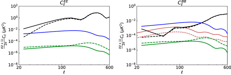
FIGURE 2. The EE and BB power spectra for the single point source simulation with given polarization direction and when r = 0.023, including the input (black solid) and filtered CMB (black dashed), residuals after the leakage removal with the ideal template (green solid) and the realistic template (green dashed), the true leakage (blue), and unlensed CMB BB spectra with r = 0.023 (red solid) and r = 0.005 (red dashed) as references. Note that the residual power spectra do not contain the contribution of the CMB.
Then we proceed to the case that the polarization direction is unknown, and construct the ideal and realistic template as explained above. In this case, the ratio of the fitting parameters kU/kQ is apparently expected to be around tan(2θ). Taking θ = 15° as an example, the result of fitting parameters, residual standard deviations and the comparison of ratios under the condition of unknown polarization direction are presented in Table 1. For both the ideal and realistic templates, kU/kQ are close to tan(2θ), with fluctuations due to the template’s chance correlation with CMB, foreground and noise.

TABLE 1. Derived fitting parameters for single point source with unknown polarization direction when r = 0.023, where the subscripts 0 and 1 denote the ideal and realistic templates, respectively.
3.2 Multiple point sources
In the case of multiple point sources for r = 0.023, five point sources are generated with random locations and are smooth with 19′. Their locations and polarization amplitudes are displayed in Table 2. The fitting parameter given by multi-linear regression for each point source is consistent to the case when the point source is treated as a single point source in simulation, as shown in Table 2; and when the polarization angles are assumed to be unknown, the fitting results are shown in Table 3. The pixel domain residuals are still 1 to 2 orders of magnitudes less than the point source’s true leakages, as shown in Figure 3.
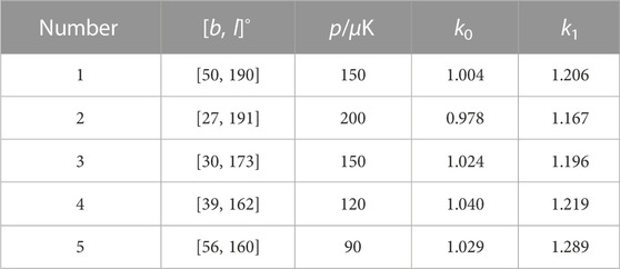
TABLE 2. Derived fitting parameters for multiple point sources by the multi-linear regression method when the polarization direction is known for each point source, which are comparable with those for each single point source.

TABLE 3. Derived fitting parameters for multiple point sources with unknown polarization direction when r = 0.023.
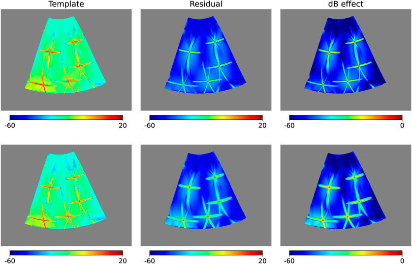
FIGURE 3. Same as in Figure 1, but for the case of multiple point sources with unknown polarization direction when r = 0.023, where the residuals are estimated through Eq. 15.
In Figure 4, we compute and compare the angular power spectrum of CMB, residuals, and true leakage for multiple point sources with unknown polarization directions. The results are similar to Figure 2 with higher residual spectra, which is consistent with expectation because more point sources are considered in simulation. After correction, the residuals’ BB spectrum is substantially smaller than the true residual’s spectrum, and also smaller than the unlensed CMB amplitude with r = 0.023 or r = 0.005 when ℓ < 200. Furthermore, as shown in Table 2, the point sources’ polarization amplitudes are apparently higher than what can be for the observation region, which means our method will actually work for a much lower tensor-to-scalar ration than r = 0.005.
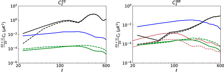
FIGURE 4. Same as in Figure 2, but for the case of multiple point sources with unknown polarization directions. The red reference spectrum are still for the unlensed CMB BB with r = 0.023 and r = 0.005, respectively.
In conclusion, our correction method maintains good accuracy and reliability for single and multiple point sources and known/unknown polarization directions, and even when the point sources’ polarization intensities are greatly overestimated. The amplitude of residuals after correction is much lower than that of the true leakage in the pixel domain; and the residual spectrum is considerably smaller than the CMB spectrum. Thus, the impact of point source leakage can be effectively corrected by our method.
3.3 Actual point sources
To simulate the actual sky map6, we use the data from 2013 Planck Catalogue of Compact Sources(PCCS). In the region we study (the same region as in Figure 3), the flux data of the 10 brightest point sources at 100 GHz are used to calculate the conversion coefficient from flux to temperature, which is equal to 2.879 μK ⋅mJy−17. The approximate temperature of these 10 brightest point sources is hence determined, and the point source polarization intensity is assumed to be 40 percent of its temperature8. Since the precise point source polarization directions are unknown before we obtain the corrected map, a set of random polarization angles are applied to simulate the input data sky map while a certain polarization direction (θ = 22.5°) is specified for each point source to build two different types of templates for simplification of calculation. For the case of r = 0.023, according to the fitting parameter results in Table 4, for both the ideal and realistic templates, the ratio of fitting parameters kU/kQ for each point source is close to tan(2θ).
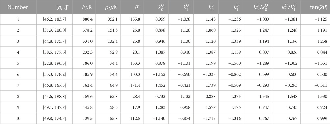
TABLE 4. Location, temperature, polarization and fitting parameter result with random polarization direction of actual 10 brightest point sources in the region we study (the region shape is the same with Figure 3) when r = 0.023.
We again build the sky map showing the polarization dB value of the templates, residuals and dB effects for actual point sources (Figure 5). The results are similar to Figure 3, as detailed in Table 5.
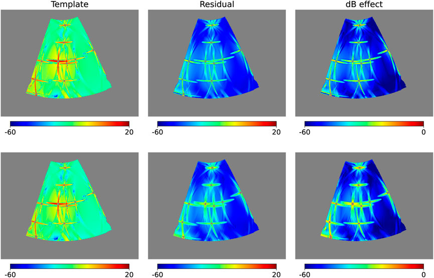
FIGURE 5. Same as in Figure 1, but for the case of actual point sources with unknown polarization direction, where the residuals are estimated using Eq. 15.
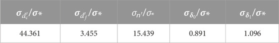
TABLE 5. Comparison of the standard deviation of σ* = 10−2 μK of filtered CMB, foreground, noise, and actual 10 brightest point sources simulation residuals with unknown polarization direction in the pixel domain when r = 0.023.
In Figure 6, with our correction method, the angular power spectrum of residual is again substantially smaller than that of the true leakage and the expected CMB signal, demonstrating the effectiveness of our method with a actual point source simulation.

FIGURE 6. Same as in Figure 2, but for the case of the actual point sources with unknown polarization directions.
4 Discussion
In this work, we have introduced a novel “template-fitting” method (Section 2) for removing the point source leakage due to time-order data filtering. The key component of this method is to create several leakage templates for each point source in the pixel domain and then fit these templates to remove the leakage contamination. Several tests for single, multi and realistic point source simulations (Section 3) are present to demonstrate the effectiveness of our method. The leakage after template fitting is typically star-like, and can be reduced by 1-2 orders of magnitude in the pixel domain and by 3-4 orders of magnitude in angular power spectrum. The performance of our method is robust in all simulations. According to the calculation of the angular power spectrum of the residuals (see Figures 2, 4, 6), we can see that the residual BB spectrum is about two orders of magnitudes lower than the theoretical prediction for the primordial gravitational waves with r ∼ 10−2 (lensed); and by comparing with the unlensed spectrum with r = 0.005 (the reference lines in Figures 2, 4, 6), we can see that our method can at least work with r = 0.005. In fact, because the polarization intensities are overestimated in all the simulations, our method should actually work with a much lower tensor-to-scalar ratio than r = 0.005, e.g., much lower than r ∼ 10−3.
The application of our template fitting method is simple with a matrix-based pipeline, and it is also preferable to use a conventional non-matrix pipeline to execute our approach, because the construction of a full matrix for a high-resolution map is infeasible at a higher resolution (scaled as
Data availability statement
The original contributions presented in the study are included in the article/Supplementary Material, further inquiries can be directed to the corresponding author.
Author contributions
All authors listed have made a substantial, direct, and intellectual contribution to the work and approved it for publication.
Funding
This work is supported by the National Key R\&D Program of China (2018YFA0404504, 2018YFA0404601, 2020YFC2201600, 2021YFC2203100, 2021YFC2203104), the Ministry of Science and Technology of China (2020SKA0110402, 2020SKA0110100), National Science Foundation of China (11890691, 11621303, 11653003), the China Manned Space Project with No. CMS-CSST-2021 (B01 \& A02), the 111 project No. B20019, and the CAS Interdisciplinary Innovation Team (JCTD-2019-05) and the Anhui project Z010118169.
Conflict of interest
The authors declare that the research was conducted in the absence of any commercial or financial relationships that could be construed as a potential conflict of interest.
Publisher’s note
All claims expressed in this article are solely those of the authors and do not necessarily represent those of their affiliated organizations, or those of the publisher, the editors and the reviewers. Any product that may be evaluated in this article, or claim that may be made by its manufacturer, is not guaranteed or endorsed by the publisher.
Footnotes
1A Gaussian beam profile is often used as an approximation.
2Strictly speaking, the point source polarization direction should also be taken into account, which will be managed in Section 3 by fitting the Q and U templates separately.
3Because the point source is affected by the filtering and the filtering is not lossless, it is theoretically impossible to fully retrieve dp. Additionally, it is impossible to completely separate point sources from CMB at the point source regions.
4Assume the point sources are non-overlapping, otherwise the summation should be replaced by the “exclusive or” (XOR) operation.
5This value is significantly higher than what could be in the region of simulation; thus, we are running the simulation with a much worse situation to estimate the lower limit of our method’s capacity.
6https://pla.esac.esa.int/#catalogues.
7Due to the different point source spectra, the standard HFI unit conversion coefficient (4.583 μK ⋅mJy−1) in the Planck 2013 result [20] can be slightly different from the value used here.
8Like above, the polarization ratio is significantly overestimated to test the performance of our method in a tough situation.
References
1. Keating BG, Ade PAR, Bock JJ, Hivon E, Holzapfel WL, Lange AE, et al. BICEP: A large angular scale CMB polarimeter. In: S Fineschi, editor. Polarimetry in astronomy. Vol. 4843 of society of photo-optical instrumentation engineers (SPIE) conference series. Amsterdam, Netherlands: SPIE (2003). p. 284–95. doi:10.1117/12.459274
2.The Planck Collaboration. The scientific programme of Planck (2006). arXiv e-prints, astro-ph/0604069.
3. Rubiño-Martín JA, Rebolo R, Tucci M, Génova-Santos R, Hildebrandt SR, Hoyland R, et al. The QUIJOTE CMB experiment. In: Highlights of Spanish astrophysics V. In: Vol. 14 of astrophysics and space science proceedings (2010). p. 127. doi:10.1007/978-3-642-11250-8_12
4. Niemack MD, Ade PAR, Aguirre J, Barrientos F, Beall JA, Bond JR, et al. ACTPol: A polarization-sensitive receiver for the atacama cosmology telescope. In: WS Holland, and J Zmuidzinas, editors. Millimeter, submillimeter, and far-infrared detectors and instrumentation for astronomy V. Vol. 7741 of society of photo-optical instrumentation engineers (SPIE) conference series. Amsterdam, Netherlands: SPIE (2010). p. 77411S. doi:10.1117/12.857464
5. Austermann JE, Aird KA, Beall JA, Becker D, Bender A, Benson BA, et al. SPTpol: An instrument for CMB polarization measurements with the south Pole telescope. In: WS Holland, and J Zmuidzinas, editors. Millimeter, submillimeter, and far-infrared detectors and instrumentation for astronomy VI. Vol. 8452 of society of photo-optical instrumentation engineers (SPIE) conference series. Amsterdam, Netherlands: SPIE (2012). p. 84521E. doi:10.1117/12.927286
6. Hinshaw G, Larson D, Komatsu E, Spergel DN, Bennett CL, Dunkley J, et al. Nine-year wilkinson microwave anisotropy probe (WMAP) observations: Cosmological parameter results. Astrophys J Suppl Ser (2013) 208:19. doi:10.1088/0067-0049/208/2/19
7.Planck Collaboration Aghanim N, Akrami Y, Ashdown M, Aumont J, Baccigalupi C, et al. Planck 2018 results. VI. Cosmological parameters (2018). arXiv e-prints, arXiv:1807.06209.
8.BICEP2/Keck CollaborationPlanck Collaboration Ade PAR, Aghanim N, Ahmed Z, Aikin RW, et al. Joint analysis of BICEP2/Keck array and planck data. Phys Rev Lett (2015) 114:101301. doi:10.1103/PhysRevLett.114.101301
9.BICEP2 CollaborationKeck Array Collaboration Ade PAR, Ahmed Z, Aikin RW, Alexander KD, et al. Constraints on primordial gravitational waves using planck, WMAP, and new BICEP2/Keck observations through the 2015 season. Phys Rev Lett (2018) 121:221301. doi:10.1103/PhysRevLett.121.221301
10. Ade PAR, Ahmed Z, Amiri M, Barkats D, Thakur RB, Bischoff CA, et al. Improved constraints on primordial gravitational waves using planck, wmap, and bicep/keck observations through the 2018 observing season. Phys Rev Lett (2021) 127:151301. doi:10.1103/PhysRevLett.127.151301
11. Keating B, Moyerman S, Boettger D, Edwards J, Fuller G, Matsuda F, et al. Ultra high energy cosmology with POLARBEAR (2011). ArXiv e-prints.
12. Hazumi M, Borrill J, Chinone Y, Dobbs MA, Fuke H, Ghribi A, et al. LiteBIRD: A small satellite for the study of B-mode polarization and inflation from cosmic background radiation detection. In: Space telescopes and instrumentation 2012: Optical, infrared, and millimeter wave. In: vol. 8442 of Proc. SPIE. Amsterdam, Netherlands: SPIE (2012). p. 844219. doi:10.1117/12.926743
13. Abazajian KN, Adshead P, Ahmed Z, Allen SW, Alonso D, Arnold KS, et al. CMB-S4 science book. 1st ed. (2016). ArXiv e-prints.
14. Ade P, Aguirre J, Ahmed Z, Aiola S, Ali A, Alonso D, et al. The Simons observatory: Science goals and forecasts. J Cosmol Astropart Phys (2019) 2019:056. doi:10.1088/1475-7516/2019/02/056
15. Li H, Li SY, Liu Y, Li YP, Cai Y, Li M, et al. Probing primordial gravitational waves: Ali CMB polarization telescope. Natl Sci Rev (2018) 6:145–54. doi:10.1093/nsr/nwy019
16. Ghosh S, Liu Y, Zhang L, Li S, Zhang J, Wang J, et al. Performance forecasts for the primordial gravitational wave detection pipelines for AliCPT-1. J Cosmology Astroparticle Phys (2022) 2022:63. doi:10.1088/1475-7516/2022/10/063
17. Liu H, Creswell J, von Hausegger S, Naselsky P. Methods for pixel domain correction of EB leakage. Phys Rev D (2019) 100:023538. doi:10.1103/PhysRevD.100.023538
18. Li H, Li SY, Liu Y, Li YP, Cai Y, Li M, et al. Probing primordial gravitational waves: Ali CMB polarization telescope. Natl Sci Rev (2019) 6:145–54. doi:10.1093/nsr/nwy019
19. Salatino M, Austermann J, Thompson KL, Ade P, Bai X, Beall J, et al. The design of the ali CMB polarization telescope receiver. In: J Zmuidzinas, and JR Gao, editors. Millimeter, submillimeter, and far-infrared detectors and instrumentation for astronomy X. Amsterdam, Netherlands: SPIE (2020). doi:10.1117/12.2560709
Keywords: cosmology, cosmic microwave background, data analysis, primordial gravitational wave, observation, cosmology
Citation: Zhang Z, Huang L, Liu Y, Li S-Y, Zhang L and Liu H (2023) Removal of point source leakage from time-order data filtering. Front. Phys. 11:1108072. doi: 10.3389/fphy.2023.1108072
Received: 25 November 2022; Accepted: 27 February 2023;
Published: 16 March 2023.
Edited by:
Taotao Qiu, Huazhong University of Science and Technology, ChinaReviewed by:
Arun Kannawadi, Princeton University, United StatesEmmanuel N. Saridakis, Baylor University, United States
Copyright © 2023 Zhang, Huang, Liu, Li, Zhang and Liu. This is an open-access article distributed under the terms of the Creative Commons Attribution License (CC BY). The use, distribution or reproduction in other forums is permitted, provided the original author(s) and the copyright owner(s) are credited and that the original publication in this journal is cited, in accordance with accepted academic practice. No use, distribution or reproduction is permitted which does not comply with these terms.
*Correspondence: Hao Liu, dXN0Y19saXVoYW9AMTYzLmNvbQ==