 Jianing Zhang
 Kexin Fang1
 Lin Zhang
95% of researchers rate our articles as excellent or good
Learn more about the work of our research integrity team to safeguard the quality of each article we publish.
Find out more
ORIGINAL RESEARCH article
Front. Phys. , 18 April 2023
Sec. Interdisciplinary Physics
Volume 11 - 2023 | https://doi.org/10.3389/fphy.2023.1107178
This article is part of the Research Topic Complex Networks in Interdisciplinary Research: From Theory to Applications View all 12 articles
Origin identification of the earliest cases during the pandemic is crucial in containing the transmission of the disease. The high infectiousness of the disease during its incubation period (no symptom yet) and underlying human interaction pattern make it difficult to capture the entire line of the spread. The hidden spreading period is when the disease is silently spreading, for the “silent spreaders” showing no symptoms yet can transmit the infection. Being uncertain of the hidden spreading period would bring a severe challenge to the contact tracing mission. To find the possible hidden spreading period span, we utilized the SEITR (susceptible–exposed–infected–tested positive–recovered) model on networks where the relation between E state and T state can implicitly model the hidden spreading mechanism. We calibrated the model with real local resurgence epidemic data. Through our study, we found that the hidden spreading period span of the possible earliest case of local resurgence could vary according to the people interaction networks. Our modeling results showed the clustering and shortcuts that exist in the human interaction network significantly affect the results in finding the hidden spreading period span. Our study can be a guide for understanding the pandemic and for contact tracing the origin of local resurgence.
Since December 2019, the newly recognized coronavirus known as severe acute respiratory syndrome–coronavirus 2 (SARS-CoV-2) has affected every individual. Globally, it has caused more than 623,000,396 confirmed cases, including 6,550,033 deaths, according to the WHO [1]. While the coronavirus has affected the healthcare system significantly, it is a greater challenge for the government to help people coordinate their daily lives living with the virus. One of the most used strategies, contact tracing, along with robust testing and isolation, is a key strategy for interrupting chains of transmission of SARS-CoV-2 and reducing COVID-19-associated mortality [1]. The virus was first reported in Wuhan, China, in late 2019. The doubt still unresolved as to when the virus actually started its spreading.
COVID-19 displays peculiar epidemiological traits when compared with previous coronavirus outbreaks [2]. A large number of transmissions occurred through human-to-human contact with individuals showing no or mild symptoms. High viral loads of SARS-CoV-2 were found in the upper respiratory samples of patients showing little or no symptoms, with a viral shedding pattern akin to that of influenza viruses [3]; hence, the inapparent transmission, that is, the disease’s hidden spread may play a major and underestimated role in sustaining the outbreak.
Origin identification requires detailed contact history records, which are not easily accessible [4]. Even now under the implemented mandatory COVID test that requires frequent detection, there is still unexpected local resurgence occurring with no clear sign. High cost and exhausted human labor are obvious problems in terms of tedious contact tracing missions, especially when the virus is rapidly evolving and there is no clear guidance on how many contacts should be isolated. The Omicron variant BA.5 remains dominant in the United States, people infected with COVID-19 can show symptoms as early as 2 days or as late as 14 days after infection, and people are generally contagious between 3 and 4 days before appearance of symptoms [5]. The BA.5 variant also causes long COVID-19 symptoms, and some can experience health problems for 4 or more weeks after first being infected [6].
To understand the complicated factors in predicting the spread of disease, stochastic mathematical epidemic modeling has been one of the main approaches in understanding the spreading dynamics of the virus. Commonly used models are SIR-inspired models, which describe the flow of individuals through three or more mutually exclusive stages of infection: susceptible, infected, and recovered. More complex models such as SEITR and SEIQR have been carried out to portray the dynamic spread of specific epidemics [7–11]. The SEITR model is a more complex and detailed infectious disease modeling framework than the SIR model [12, 13]. The SEITR model includes a more accurate representation of disease progression and allows for a better understanding of the transmission dynamics of the disease. It accounts for the latency period between exposure and onset of symptoms and can help in modeling diseases where individuals can spread the infection before showing symptoms [14].
In order to understand the local resurgence and find the possible hidden spreading period, we utilized a modified SEITR (susceptible–exposed–infected–tested positive–recovered) compartmental mathematical model for predictions of COVID-19 epidemic dynamics. Our main goal is to use the modified SEITR model to trace back the origin time of the spreading process, given a certain number of confirmed cases. In the following article, real local resurgence data from Xi’an, China, is used to calibrate the model to find the possible hidden spreading period of local resurgence. While homogeneous contact is not applicable in real life, we compared our model on different people interaction networks to observe the impact of clustering and shortcuts created by mobility. Our results showed that the existence of clustering and shortcuts does affect the speed of disease transmission, hence affecting our decision in finding the possible hidden spreading period span. Although local resurgence seems unpredictable, our model provides guidance for time spans of contact tracing and suggestions on modifications of control measures and testing abilities.
The SEITR model is a variation of the basic SIR (susceptible–infectious–recovered) model used for modeling the spread of infectious diseases in a population [14]. The SEITR model includes additional compartments to account for more complex disease transmission dynamics. Considering one population, as shown in Figure 1, the model subdivides the total human population size at time t denoted as N(t) into susceptible S(t), exposed E(t), infected I(t), tested positive T(t), and the recovered R(t). Hence, for the population, we have N(t) = S(t) + E(t) + I(t) + T(t) + R(t).
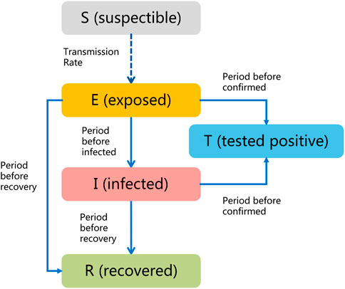
FIGURE 1. SEITR model transmission graph.
Since the beginning of the COVID-19 epidemic, SARS-CoV-2 has evolved and mutated continuously, producing variants with different transmissibility and virulence. Real data indicate that asymptomatic and symptomatic infected individuals can spread the virus to susceptible persons through close contact. Mwalili identified the difference between asymptomatic and symptomatic infected individuals by dividing the infected I(t) into these two subpopulations. Ottaviano provides analytical results for SAIRS (susceptible–asymptomatic infected–symptomatic infected–recovered–susceptible) model where asymptomatic infected is considered one compartment [15, 16]. While different approaches have been taken in considering the “silent spreaders”—those showing no symptoms and able to transmit the infection—here in our study, we included both the concept of incubation period along with the asymptomatic infected individuals into the compartment exposed E(t). The hidden spreading period Φ is when the disease is silently spreading, for the “silent spreaders” showing no symptoms yet able to transmit the infection, and the uncertainty of the hidden spreading period would bring a severe challenge to the contact tracing mission. We define the hidden spreading period Φ as the time since the initial infectious individual [exposed individual E(t) or infected individual I(t)] in the population until the time since the first confirmed case T(t). In the process of disease spread, the susceptible individual first moves to the exposed population E(t) when making contact with exposed or infected individuals since they both are infectious. During the incubation period, the exposed population may develop severe symptoms like shortness of breath, chest pain, or confusion [these would move to the infected population I(t)], some may be self-immune to the virus [move to recovered R(t)], and some people may only have very mild or non-specific symptoms [some can be tested as confirmed cases T(t)]. T(t) is the number of confirmed cases detected through the ordinary COVID tests at time t; this number can be significantly affected by the testing ability. Some infected individuals would be detected positive through ordinary screening, and some infected individuals would self-recover and move to the recovered human population R(t).
The SEITR model is, thus, governed by the reactions:
where parameters used in the transmission model are given in Table 1.
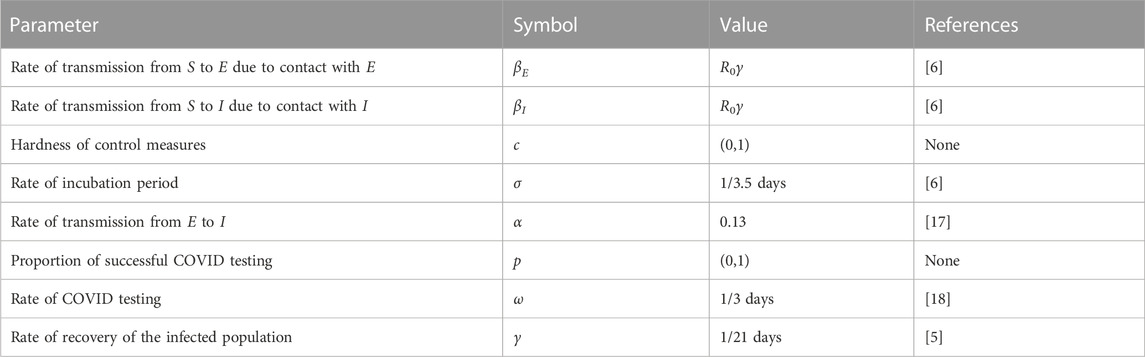
TABLE 1. Model parameters.
The contagion process involves contact interaction. In this mean field approach, the effect of contact on susceptible individuals with exposed and infected individuals is considered in a homogeneously mixed population. So, the model culminates in the following systems of mean field equations:
The basic reproduction number defines the average number of secondary infections caused by an individual in an entirely susceptible population. The derivation of R0 in our model can be approximated by R0 = βI/γ. There is no death or birth in the process, and an individual would attain immunity after recovery and cannot be infected again.
During the hidden spreading period, the exposed population spread the virus “silently,” wherein some would self-recover, some would transfer to infected individuals, and some would be detected as test positives. Real data showed that the transmission rate from asymptomatic to infected individuals during local resurgence in Shanghai in April is 1995/15284 = 13.05% [17]. In the model, βI and βE are generated from R0∗γ, which is around 0.88. 1/σ is the average latency period of the exposed individuals and 1/γ captures the average recovery time of the infected population.
In the model, two aspects of non-pharmaceutical intervention practices are introduced to model the effect of intervention policies. In facing a local resurgence of the disease, the hardness of control measures c ∈ (0, 1) would be tightened to scale down the ability of transmission. This act could be explained by reduced contact interaction during city lockdown or suspended travel activities. For other non-pharmaceutical intervention practices, the testing ability would affect the number of tested positive T(t) individuals, which consist of two latent parameters: rate of successful COVID testing p ∈ (0, 1) and testing frequency ω. Depending on the quality of each throat swab, the rate of successful COVID testing p would vary and rely highly on those third-party organizations corresponding to the testing. The testing frequency ω describes how frequently the COVID test is implemented. The current standard in major cities for testing frequency is a COVID test in 3 days and one test per day during lockdowns.
Considering the aforementioned interaction measures, our model can capture the dynamics of the spreading process when restrictions are implemented during a local resurgence.
The data used to calibrate the model were real local resurgence data from Xi’an, China, from 09 August 2022 to 18 September 2022 [18]. The first BA.5 confirmed case was detected on August 9 in Xi’an, which then caused rapid increase in daily new cases, consisting daily new infected cases and daily new asymptomatic cases. In our simulation, we implemented the lockdown once the number of tested positive T(t) exceeds 18 by minimizing the control measure c to 0 and pushing the testing ability p to the highest 0.99 with a daily COVID test, as what really happened in July at Xi’an. The source of this local resurgence was still not clear.
The methodology of locating the earliest case in local resurgence is as follows: first, real data are used to calibrate the SEITR model, and then the control policies are added. This can be done by adjusting only control measures (c), rate of successful COVID testing (p), and testing frequency (w), while the remaining parameters are determined by real clinical report data. Since these parameters act directly on the transmission of the disease, different combinations of the aforementioned policy measures can simulate different control scenarios such as city lockdowns and restrictions on human travel. Normally in real life scenarios, control policies would be strengthened once the newly confirmed cases exceed a certain number. However, it is certain that the disease has been spreading hidden for a period, and this is why finding the possible hidden spreading period Φ span is crucial for the following contact tracing work.
A total population of N = 13, 000, 000 is considered to approximate the population of Xi’an city. As shown in Figure 2, initially, we added one infected (I) individual into the population, while the remaining population are susceptible (S) individuals. We can clearly see that even days before disease detection, a certain number of exposed (E) individuals in the population have been “silently” spreading the virus. During this hidden spreading period Φ, some exposed individuals are already infectious, yet due to the virus being still in its incubation period, they may escape from detection. The rapid increase in the number of either tested positive (T) or recovered (R) would occur once it is detectable or recovered, respectively. With the implementation of the lockdown, restrictions in control measures such as less travel or visiting (c = 0.4) and increasing the testing ability and the frequency (p = 0.99, w = 1), the increase in the confirmed case would soon reduce as what happened in Xi’an.
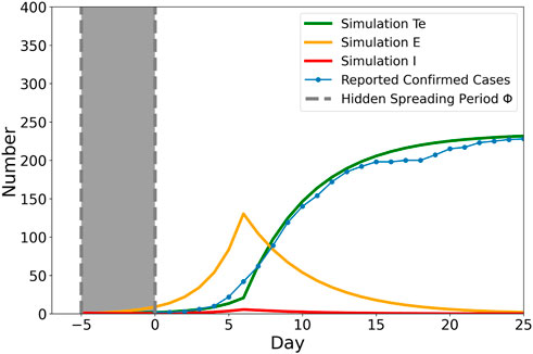
FIGURE 2. Simulation result with real Xi’an local resurgence data fitted. The blue dotted line shows the real recorded accumulated daily confirmed cases since Day 0. The green line is the simulated tested positive number with the implementation of lockdown once the number of reported confirmed case exceeds 40. βI = βE = 0.88, c = 1, w = 1/3, p = 0.8. The shaded area Φ = 5 hidden spreading period span was added to the real data to capture the delay of growth in simulation, indicating the possible initial infected individual started its hidden spreading period around 5 days ago.
The hidden spreading period Φ is deduced by comparing the difference between the first reported case in real resurgence record and the simulated initial spreader. As shown in Figure 2, the shaded area Φ = 5 hidden spreading period span was added to the real data to capture the delay of growth in simulation, indicating the possible initial infected individual started its hidden spreading period around 5 days ago. We define
The mean field numerical results can provide us with the solution to the systems of equations; however, the real-case scenario is much more complicated than one system of equations. Φ = 5 is the most possible hidden spreading period based on the strong assumption that the population is homogeneously mixed. However, in real life, social interactions are much more complicated, and the heterogeneity in human behavior would significantly affect the speed of transmission. The key to confronting the pandemic is to lower the rate of transmission of the disease. Our non-pharmaceutical intervention practice parameters in the model can provide a vague picture of modifying the transmission rate. Having c = 0 (city lockdown) is one of the worst-case scenarios since it bans people from moving.
Therefore, it is necessary to understand the trade-offs between restrictions and daily activities. Some regulations such as restricting certain types of transportation would decrease human mobility; hence, in turn, lowering the transmission rate may also be useful, but is it really efficient in controlling the spread of the disease? In the following section, we extended our model on human interaction networks to discuss the impact of clustering and shortcuts created by mobility.
Many studies have shown that human daily interactions and mobility can lead to construction of local communities and shortcuts in social networks [19]. Clustering is often simply described as the number of triangles (where the friend of my friend is also my friend) in a network, but usually also implies that links between nodes tend to be aggregated in well-connected, groups as shown in Figure 3. Hebert–Dufresne investigated the impact of contact structure clustering on the dynamics of multiple diseases interacting through the coinfection of a single individual and found the opposite effect of clustering. In addition, they showed that although clustering slows down the propagation of non-interacting diseases, it would speed up the propagation of synergistically interacting diseases [20].
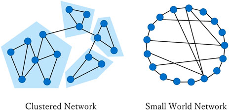
FIGURE 3. Different network structure.
Extensive studies on mobility within the pandemic revealed that population mobility is among the main drivers of the spatial spreading of the outbreak [19, 21, 22]. The complex social network structures created by heterogeneous mobility and contacts would affect the spread of the disease significantly [21]. At the modeling level, the network consists of a set of communities (node), connected by edges that capture daily short-range commuting and long-range mobility. The small-world network is one of the most basic representations of human interaction patterns in network science, by analogy with the small-world phenomenon [23]. We run our model on simple small-world networks by modifying initial rewiring probability to simulate the existence of shortcuts, an analogy of the shortcuts created by travel behavior.
The community structure network extended the description of propagation dynamics on a highly clustered network using overlapping community structures [20]. The arrangement of nodes leads to clustering of nodes into well-connected groups, which may represent the notion of a workplace or family. Every connection in this structure can be decomposed in terms of groups, where even single links between two individuals can be considered a group of size 2. Assuming that we know the distribution of group sizes (number of nodes per group) and of node memberships (number of groups per node), we can define a maximally random ensemble of clustered networks with a fixed community structure by randomly assigning nodes to groups. Hence, the entire network structure is solely defined by two probability distributions, pn, and gm, respectively, which are the probabilities that a randomly selected group will contain n members (size n) or that a randomly selected individual will participate in m groups (m memberships). This concept results in a network with highly connected communities and a sparser density of links between them. To highlight the effects of community structure (CS), an equivalent random network (RN) with exactly the same degree distribution but randomly rewired links is generated. Furthermore, description of the dynamics of the community structure can be found at [20].
The network-based SEITR model counts the changes in network contacts upon the presence of infected (I) and also allows for exposed (E), which could be used to simulate the likely changes in contact patterns of an individual in tested positives. The parameters discussed in previous sections are preserved during the Monte Carlo simulation. The one seed-infected individual was added randomly into the network of 2,000 nodes. At each time step, susceptible individuals Si would be infected and transmit to exposed Ei when contacted with exposed individual Ej or infected individual Ij neighbors. The transmission rate could be expressed as β = 1 − ∑j∈[1,N](1 − βEEj)(1 − βIIj)Aij, while A is the adjacency matrix of the network. During the incubation period, exposed individuals would transfer to infected individuals spontaneously, and some would self-recover. In both exposed and infected individuals, some would be detected as tested positive Ti. By modifying the control measures and test ability, we would see how these non-pharmaceutical intervention practices affect the time tracing of the earliest case.
We tested our model on both the community structure network and the equivalent random network introduced by Hebert–Dufresne [20], hoping to find the evidence of clustering speed up the propagation and hence influence our decision in finding the Φ hidden spreading period span. In addition, since the network models described by Hebert–Dufresne mainly focused on the effect of the existence of clustering, we also discussed the effect of the shortest path created by human mobility in the network. We addressed this by running the model on a small-world network, modifying the probability of rewiring an edge [23].
The existence of community is a common feature of human interaction networks. The main goal of running the SEITR model on different network structures is to reconstruct the possible human interaction networks during disease propagation. Figure 4 shows the phase diagram of running simulation on the community structure network and the equivalent random network shows the number of tested positive (T) at its final steady state of each simulation. The control measures c and frequency of COVID test w are two non-pharmaceutical intervention practices that can be modified in our model to simulate real intervention conditions. Lower c means a lower level of transmission, and higher c means there are no restrictions to prevent the disease from spreading. The lowest frequency of COVID testing w means no COVID test is conducted; hence, all the exposed and infected individuals would remain in the population and spread the disease silently. Assuming a 100% success in COVID testing p = 1, we compared how the two intervention policies would affect the propagation. As shown in Figure 4, w = 0 means no COVID test is conducted; hence, no test positive exists in the population; w = 1 means any exposed or infected individuals would be detected once they are positive. Figure 4A shows the number of tested positive (T) at its final steady state on the community structure network of the 2,000 nodes. In Figure 4B, the equivalent random network result is presented. The random network is created from the community structure network, by randomly rewiring the links within the community to another node while keeping the same average degree. The resulting random network in our analysis has a clustering coefficient of around 0.05, while the coefficient of the structure community network is around 0.10. In Figure 4, we can see that although the average degree of both networks is relatively the same, the changes in the community structure network are smoother than those of the random network due to the randomness of Monte Carlo simulations. There are similarities between community structure and its equivalent random network, and the reason may be how the community structure network was constructed. Although the clustering coefficient is doubled for the community structure network, the relatively same average degree and average shortest path of the two networks would smooth out the effect of clustering on disease propagation. However, if we focus on a coarse-grained level of the heat map, the combined influence of the two intervention policies on disease transmission is clear and would be useful as guidance.
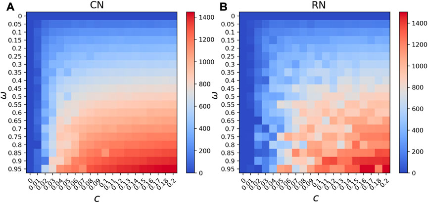
FIGURE 4. Phase diagram of steady state tested positives (T) (A) on the community structure network and (B) the equivalent random network under different combinations of control measures and testing frequency.
While the phase diagram provides thorough information about how the combined intervention would affect the results of the disease spread, our main task is to locate possible hidden spreading period span Φ in a local pandemic resurgence. Through each simulation, we counted the number of days needed for a local resurgence, and the accumulated tested positive number exceeds 10. As shown in Figure 5, we provided a comparison between different community structures by varying its clustering coefficient C. With the increased clustering coefficient, the hidden spreading period span would shrink significantly, indicating that a higher clustering network provides a smaller hidden spreading period span Φ. We can conjecture that the clustering in the network does affect the speed of the propagation. As shown in Figure 5A, with a daily COVID test window, all the positives would be detected immediately. As shown in Figure 5B, a higher clustering coefficient of 0.6 would still provide a shorter span than that of a clustering coefficient of 0.2 and 0.4. In addition, Figure 6A shows the trend of how the average hidden spreading period span changes along with different clustering coefficients. The red line represents the result of Φ if the COVID test is conducted per week; it is obvious that a delayed test would shade the hidden spreading and, hence would cause more difficulty in conducting the contact tracing. Especially in the low clustering region (clustering coefficient of 0.05), a 1-week delayed test would lead up to 1 month of contact tracing. If the test is not conducted daily, but with a delay of few days, some exposed and infected individuals would self-recover, and some would still spread the disease ‘silently’ and not be tested on time. This is the reason the hidden spreading period spans are increased, hence increasing the tracing back time of the origin of disease propagation.
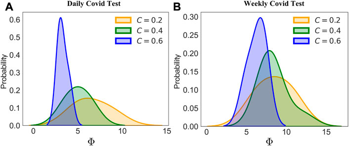
FIGURE 5. Probability density distribution of the hidden spreading period span Φ. Holding a control measure of c = 0.03, two testing frequencies are chosen, a test per day (A) and a test per 7 days (B). Results under different clustering coefficient community structure networks (CNs) are provided.
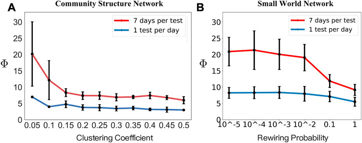
FIGURE 6. Hidden spreading period span Φ results. Holding a control measure of c = 0.03, two testing frequencies are chosen, a test per day (blue lines) and a test per 7 days (red lines). (A) A set of community structure networks has different clustering coefficients. (B) Small-world network with six sets of rewiring probability were chosen, providing the average shortest path from 20.49, 11.58, 5.58, 3.43, 2.72, and 2.25, respectively.
The time span results may vary according to the heterogeneity of human interaction behaviors. We showed the existence of a community provides a higher amount of interactions in the community, and the disease would spread faster, hence reducing the hidden spreading period span. Another effect of human interaction networks is the existence of a short path in the network. In our daily activities, a short journey to another city can create a short path for the contagious disease. To address the influence of human travel, we used the small-world network developed by Watt and Strogatz [23]. The network of 2,000 nodes has an average degree of 50, representing the number of people that an individual has regular physical contact with, e.g., family members, co-workers, and friends. We compared different sets of rewiring probability p, the probability that an edge is disconnected from one of its nodes and then randomly connected to another node anywhere in the network (vertex may have a long-range shortcut connected to a remote vertex).
As shown in Figure 6B, six sets of rewiring probability were chosen, providing different average shortest paths. Similar to that shown in Figure 6A, the trend of both lines steadily decreases, indicating a smaller average shortest path provides a shorter period of hidden spreading span. In general, the daily COVID test would capture both exposed and infected individuals immediately, but with delayed testing, the span of the possible period distribution would be increased. Through the aforementioned comparison, we conclude that the structure of how human interaction networks would have a great influence on how fast disease propagation is, and in turn, influence the time tracing mission finding the origin of the propagation.
It should be necessary to point out that rewiring probability p is meaningful only in a relative sense. For example, choosing a degree of 50 and p = 0.01 does not imply that each person in society interacts with 50 people in daily activities and knows only one person in far-away areas. But rather, the changes from p = 0.01 to p = 0.001 mean that, on average, each person reduces the daily infection-transmissible interactions by half and/or long-distance travel by 90%. Another point that needs to be made is that in real-world social networks, different individuals have different ways of interacting with others, for example, the contact frequency is usually different between the different contact patterns, and household contact is significantly more frequent than other scenarios. For example, it is unknown how individuals with different levels of social interactions respond to social distancing or lockdown orders. Figure 7 shows that different choices of the contact frequency distribution do not affect greatly tracing the possible hidden spreading span. In our study, the contact frequency is assumed to be the same for all the vertices because there is no adequate data on the real contact network. So in order to address the problem of the heterogeneity of contact frequency, except for the constant control measure c, we also tested both power-law distributed contact frequency and uniformly distributed contact frequency. Holding the mean of the distribution to the same constant number, we see no clear difference in finding the possible hidden spreading period. Hence, the use of the constant contact frequency with each individual represented as a vertex can still provide useful predictions.
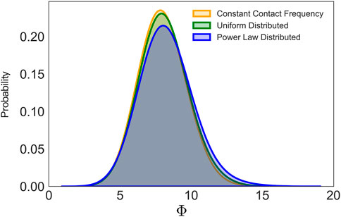
FIGURE 7. Probability density distribution of the possible hidden spreading span under the different choice of contact frequency. Holding the mean of the contact frequency as 0.05, we compared the influence of contact frequency on the possible hidden spreading span.
Till today, SARS-CoV-2 has caused more than 623,000,396 confirmed cases, including 6,550,033 deaths. We need to understand how and what should we do to live with the disease. Origin identification of the earliest cases during the pandemic is crucial in terms of contact tracing. It is a key strategy for interrupting chains of transmission of SARS-CoV-2 and reducing COVID-19-associated mortality. However, high cost and human labor are a problem in terms of contact tracing, especially when the virus is rapidly evolving and there is no clear guidance on how many contacts should be isolated. To help understand the disease propagation and to trace the earliest case, we utilized a modified SEITR compartmental mathematical model for prediction of COVID-19 epidemic dynamics. Our main goal was to use the data-driven simulation result to find the possible hidden spreading period span since the beginning of the spreading process. Real local resurgence data of Xi’an, China (August 2022) were used to fit the mean field model. Our result indicated the possible initial infected individual started its hidden spreading period around 5 days ago since the first recorded confirmed case.
Since a homogeneously mixed population is not applicable in real life, we then tested our model on different network structures to simulate human interaction patterns. The community structure network extended the description of propagation dynamics on a highly clustered network using overlapping community structure [20], and our results showed that in a local pandemic resurgence, given a certain amount of test positive cases, a high clustering network does minimize the possible hidden spreading span. We then discussed the effect of the short path created by human mobility. The results showed clear evidence that shorter average paths provide a shorter period of the hidden spreading results. In real-case scenarios, these together may infer the different human interaction patterns between big cities and rural areas. Where communities are very common and have constant interactions with remote individuals, a local resurgence in big cities always appears very suddenly and breaks out. If not with accurate control restrictions, a larger pandemic seems inevitable. However, in rural areas, where communities are normally sparse and lack interactions, the local resurgence is not very often and may not grow to a larger scale. Hence, in order to capture the “silent” spreaders in a timely manner, accurate contact tracing should be carried out as soon as a positive is detected to avoid further costs.
We discussed two aspects of non-pharmaceutical intervention practice in facing the local resurgence of the disease. The hardness of control measures scales down the ability of transmission and testing ability, consisting of the rate of successful COVID testing and testing frequency. Control measures could be interpreted as the restrictions policies such as city lockdowns, while the testing ability represents the detection quality. Based on these, our model provides insights into how the combination of the interventions could affect the speed of disease propagation. Our results present the possible distribution of the hidden spreading period span in terms of contact tracing.
There is a certain amount of mis-considerations when building up our SEITR model, for example, the birth and death rate of the population is not included, as well as the quarantine factor. The network structures we considered were all static rather than temporal. In real life, the spontaneous and temporal movement could modify human interaction networks. More studies need to be performed to address the real changing temporal characteristics of human mobility to better understand the propagation patterns. In addition, our study of disease propagation could also extend to subjects such as idea propagation [24–26], culture spreading [27], and signal propagation [28]. For example, signal propagation patterns on complex networks may be helpful in understanding the complex behavior of the contagion, especially how the social system would respond according to perturbation of the dynamics [28, 29]. Our work put forward the method to timing the earliest case, given real local resurgence data. Although local resurgence seems unpredictable, our model provides a guidance for time spans of contact tracing as well as suggestions on modifications of control measures and testing abilities.
The datasets presented in this study can be found in online repositories. Epidemiological data for this study are available at http://www.nhc.gov.cn/xcs/yqtb/list_gzbd.shtml. The code used for the simulations is available at https://github.com/avecsally/Tracing-the-time-of-the-origin-in-local-epidemic-spreading-on-networks/tree/main.
JZ, KF, and LZ conceived and designed the research with inputs from all the authors. JZ and KF performed parameter identification and the numerical studies and wrote the first draft of the manuscript. JZ and LZ supervised the research and consolidated the manuscript in its present submission. JZ contributed to the interpretation and analysis of the results and to reviewing the current submission of the manuscript. All authors contributed to the article and approved the submitted version.
This work was jointly supported by the National Natural Science Foundation of China (Grant Nos. 11971074 and 61671005).
The authors declare that the research was conducted in the absence of any commercial or financial relationships that could be construed as a potential conflict of interest.
All claims expressed in this article are solely those of the authors and do not necessarily represent those of their affiliated organizations, or those of the publisher, the editors, and the reviewers. Any product that may be evaluated in this article, or claim that may be made by its manufacturer, is not guaranteed or endorsed by the publisher.
1.World Health Organization. Contact tracing in the context of covid-19. interim guidance. Pediatria i Medycyna Rodzinna (2020). Available at: https://www.who.int/emergencies/diseases/novel-coronavirus-2019/global-research-on-novel-coronavirus-2019-ncov.
2. Giordano G, Blanchini F, Bruno R, Colaneri P, Filippo AD, Matteo AD, et al. Modelling the Covid-19 epidemic and implementation of population-wide interventions in Italy. Nat Med (2020) 26:855–60. doi:10.1038/s41591-020-0883-7
3. Read JM, Bridgen JR, Cummings DAT, Ho AYW, Jewell CP. Novel coronavirus 2019-ncov: Early estimation of epidemiological parameters and epidemic predictions. medRxiv (2020). Philosophical Transactions of the Royal Society B.
4. Xia Y, Lee G. How to return to normalcy: Fast and comprehensive contact tracing of covid-19 through proximity sensing using mobile devices (2020). arXiv preprint. ArXiv:2004.12576.
5.CDC. Nsars-cov-2 variant classifications and definitions. Centers for Disease Control and Prevention (2022). Available at: https://www.cdc.gov/coronavirus/2019-ncov/variants/variant-classifications.html.
6.UC DAVIS HEALTH. Omicron ba.5: What we know about this covid-19 strain (2023). Available at: https://health.ucdavis.edu/coronavirus/covid-19-information/omicron-variant.
7. Prabakaran R, Jemimah S, Rawat P, Sharma D, Gromiha MM. A novel hybrid seiqr model incorporating the effect of quarantine and lockdown regulations for Covid-19. Scientific Rep (2021) 11:24073. doi:10.1038/s41598-021-03436-z
8. Huang Q, Ma J, Xu Z, Gu X, Yang M. A staging prediction model for Covid-19 pandemic under strong public health interventions. In: 2022 Tenth International Conference on Advanced Cloud and Big Data (CBD); 04-05 November 2022; Guilin, China (2022). p. 184–9. doi:10.1109/CBD58033.2022.00040
9. Yang Z-F, Zeng Z, Wang K, Wong S-S, Liang W, Zanin M, et al. Modified seir and ai prediction of the epidemics trend of Covid-19 in China under public health interventions. J Thorac Dis (2020) 12:165–74. doi:10.21037/jtd.2020.02.64
10. Cai M, Karniadakis GE, Li C. Fractional seir model and data-driven predictions of Covid-19 dynamics of omicron variant. Chaos (2022) 32:071101. doi:10.1063/5.0099450
11. Calafiore GC, Novara C, Possieri C. A modified sir model for the Covid-19 contagion in Italy. In: 2020 59th IEEE Conference on Decision and Control (CDC); 14-18 December 2020; Jeju, Korea (South) (2020). p. 3889–94. doi:10.1109/CDC42340.2020.9304142
12. Kucharski AJ, Russell TW, Diamond C, Liu Y, Edmunds JW, Funk S, et al. Early dynamics of transmission and control of Covid-19: A mathematical modelling study. Lancet Infect Dis (2020) 20:553–8. doi:10.1016/s1473-3099(20)30144-4
13. Hethcote HW. The mathematics of infectious diseases. SIAM Rev (2000) 42:599–653. doi:10.1137/s0036144500371907
14. Brauer F, Castillo-Chavez C. Mathematical models in population biology and epidemiology New York: springe (2001) 2:40.
15. Mwalili S, Kimathi M, Ojiambo V, Gathungu D, Mbogo R. Seir model for Covid-19 dynamics incorporating the environment and social distancing. BMC Res Notes (2020) 13:352. doi:10.1186/s13104-020-05192-1
16. Ottaviano S, Sensi M, Sottile S. Global stability of sairs epidemic models. Nonlinear Anal Real World Appl (2022) 65:103501. doi:10.1016/j.nonrwa.2021.103501
17.Hangzhou. Hangzhou (2022). Available at: https://news.hangzhou.com.cn/gnxw/content/2022-04/15/content_8228338.htm (Accessed on 04 15, 2022).
18.NHC. NHC (2022). Available at: http://www.nhc.gov.cn/xcs/yqtb/list_gzbd.shtml (Accessed on 11 13, 2022).
19. Parino F, Zino L, Porfiri M, Rizzo A. Modelling and predicting the effect of social distancing and travel restrictions on Covid-19 spreading. J R Soc Interf (2021) 18:20200875. doi:10.1098/rsif.2020.0875
20. Hébert-Dufresne L, Althouse B. Complex dynamics of synergistic coinfections on realistically clustered networks. Proc Natl Acad Sci United States America (2015) 112:10551–6. doi:10.1073/pnas.1507820112
21. Kraemer MUG, Yang C-H, Gutierrez B, Wu C-H, Klein B, Pigott DM, et al. The effect of human mobility and control measures on the Covid-19 epidemic in China. Science (2020) 368:493–7. doi:10.1126/science.abb4218
22. Jia J, Lu X, Yuan Y, Xu G, Jia J, Christakis N. Population flow drives spatio-temporal distribution of Covid-19 in China. Nature (2020) 582:389–94. doi:10.1038/s41586-020-2284-y
23. Watts D, Strogatz S. Collective dynamics of small world networks. Nature (1998) 393:440–2. doi:10.1038/30918
24. Watts DJ. A simple model of global cascades on random networks. Proc Natl Acad Sci United States America (2002) 99:5766–71. doi:10.1073/pnas.082090499
25. Granovetter MS. Threshold models of collective behavior. Am J Sociol (1978) 83:1420–43. doi:10.1086/226707
26. Leskovec J, Adamic LA, Huberman BA. The dynamics of viral marketing. ACM Trans Web (2005) 1:5. doi:10.1145/1232722.1232727
27. Kempe D, Kleinberg JM, Tardos É. Maximizing the spread of influence through a social network. In: Knowledge discovery and data mining (2003).
28. Bao X, Hu Q, Ji P, Lin W, Kurths J, Nagler J. Impact of basic network motifs on the collective response to perturbations. Nat Commun (2022) 13:5301. doi:10.1038/s41467-022-32913-w
Keywords: SEITR, resurgence, origin identification, tracing, EPI, epidemiology
Citation: Zhang J, Fang K, Zhu Y, Kang X and Zhang L (2023) Time tracing the earliest case of local pandemic resurgence. Front. Phys. 11:1107178. doi: 10.3389/fphy.2023.1107178
Received: 24 November 2022; Accepted: 30 March 2023;
Published: 18 April 2023.
Edited by:
Ye Wu, Beijing Normal University, ChinaReviewed by:
Zhongyuan Ruan, Zhejiang University of Technology, ChinaCopyright © 2023 Zhang, Fang, Zhu, Kang and Zhang. This is an open-access article distributed under the terms of the Creative Commons Attribution License (CC BY). The use, distribution or reproduction in other forums is permitted, provided the original author(s) and the copyright owner(s) are credited and that the original publication in this journal is cited, in accordance with accepted academic practice. No use, distribution or reproduction is permitted which does not comply with these terms.
*Correspondence: Lin Zhang, emhhbmdsaW4yMDExQGJ1cHQuZWR1LmNu
Disclaimer: All claims expressed in this article are solely those of the authors and do not necessarily represent those of their affiliated organizations, or those of the publisher, the editors and the reviewers. Any product that may be evaluated in this article or claim that may be made by its manufacturer is not guaranteed or endorsed by the publisher.
Research integrity at Frontiers
Learn more about the work of our research integrity team to safeguard the quality of each article we publish.