 Yan Li
 Sisi Xu2†
 Yao Lu
 Zhenyu Qi
95% of researchers rate our articles as excellent or good
Learn more about the work of our research integrity team to safeguard the quality of each article we publish.
Find out more
ORIGINAL RESEARCH article
Front. Phys. , 23 January 2023
Sec. Medical Physics and Imaging
Volume 11 - 2023 | https://doi.org/10.3389/fphy.2023.1088899
This article is part of the Research Topic Artificial Intelligence for Medical Informatics View all 8 articles
Introduction: Using MRI to synthesize CT and substitute its function in radiation therapy has drawn wide research interests. Currently, deep learning models have become the first choice for MRI—CT synthesis because of their ability to study complex non-linear relations. However, existing studies still lack the ability to learn complex local and global MRI–CT relations in the same time , which influences the intensity and structural performance of synthetic images.
Methods: This study proposes a hybrid multi-scale model to explore rich local and global MRI—CT relations, relations, namely, the hybrid multi-scale synthesis network (HMSS-Net). It includes two modules modelling different resolution inputs. In the low-resolution module, the Transformer method is applied to build its bottleneck part to expand the receptive field and explore long-range MRI—CT relations to estimate the coarse distribution of widely spread tissues and large organs. In the high-resolution module, residual and dense connections are applied to explore complex local MRI—CT relations under multiple step sizes. Then, the feature spaces of two modules are combined together and utilized to provide synthetic CT. HMSS-Net also introduces the multi-scale structural similarity index measure loss to provide multi-scale supervision during training.
Results: The experimental results on head and neck regions of 78 patients showed that HMSS–Net reduced the average of 7.6/3.13 HU on the mean absolute error and increased the average of 2.1/1.8% on the dice coefficient of bone compared with competing image–to–image synthesis methods.
Conclusion: The results imply that HMSS–Net could effectively improve the intensity and structural performances of synthetic CT.
Magnetic resonance imaging (MRI) is an important medical imaging modality as it presents a clear soft-tissue structure of the human body without introducing ionizing radiations like in computed tomography (CT) [1]. Currently, MRI is widely used in clinical diagnosis and tumor or organ delineation. However, since MRI cannot reflect the electron density of the human body, CT is still essential in the current radiation therapy (RT) workflow for a dose plan [2]. For increasing the efficiency of RT and prevent additional ionizing radiation to patients, studies were carried out to investigate the possibility of using MR images to synthesize CT and replace its function in RT [3].
In recent years, deep learning (DL) has become the first choice for MRI–CT synthesis because deep network models have the ability to study complex non-linear relationships [4]. An early study by Han et al. [5] used a deep convolutional neural network (CNN) model to synthesize CT from MRI with pretrained VGG weights as initialization, and their work proved that the DL-based method is a feasible solution to MRI–CT synthesis. With the rapid development of DL, researchers began to introduce more complex frameworks and powerful models to this task. For example, as Han’s work only applied L1-loss to measure the distance between synthetic and real CT that tends to produce blurry results, the generative adversarial network (GAN) was applied to add authenticity and detailed patterns to synthetic CT images in the study of Dong et al. [6]. Maspero et al. [7] further introduced a conditional GAN model called ‘pix2pix’ that pays more attention on high-frequency features to improve the performance on local structures. While the aforementioned studies are trained under registered MRI–CT data, the CycleGAN framework was introduced in the work of Wolterink [8] to provide unpaired training for the affection of the MRI–CT registration error. However, owing to the lack of constraints, unpaired training is difficult to preserve structural consistency between synthetic and real CT; hence, Yang et al [9] proposed a structure-consistency loss function in their study to solve this problem. Meanwhile, with the concept of ‘more modality brings more information’, some researchers turned to collect multiple MRI sequences to synthesize CT [10, 11]. The study of Mengke et al. [11] thoroughly analyzed the performance of using four MRI sequences together with a multi-channel pix2pix model. In addition to the overall framework, there are studies focusing on detailed network structures. For example, Haley [12] applied the Inception V3 [13] block to replace the conventional convolutional block, which could aggregate convolutions under various kernel sizes together and study different types of patterns. Dinkla [14] introduced the dilated convolution to MRI–CT synthesis to enlarge the receptive field of the model for studying contextual correlations between different regions.
Although aforementioned studies obtained considerable results, they have the limitation of learning multi-scale MRI–CT relations. Considering the intensity and structure of a CT image are both essential to calculate the attenuation of X-ray beams inside a patient’s body, both local and global properties of CT should be well-synthesized. In more recent cross medical-imaging synthesis studies, such a problem has been addressed by introducing a multi-scale learning framework. For example, the work of Boni et al. [15] introduced the ‘pix2pixHD’ model for MRI–CT synthesis, which is a multi-scale version of pix2pix. It contains two synthesis modules to model the low-resolution and high-resolution inputs to extract global and local relations, respectively. According to the results, pix2pixHD successfully outperformed pix2pix on the performance of synthetic CT. In another work was by Xuzhe et al. [16], the authors designed a multi-scale transformer-based model for cross-MRI synthesis. However, as convolution is efficient to extract local image patterns and the transformer focuses more on long-range image patterns [17], pure convolution- or transformer-based models could not utilize the strength of the other method.
In this study, we propose a hybrid multi-scale model for MRI–CT synthesis aiming to explore rich local and global MRI–CT relations, which is called the hybrid multi-scale synthesis network (HMSS-Net). HMSS-Net has two synthesis modules for pyramidal inputs like pix2pixHD, but each module has a different design targeting at the local or global information. Specifically, in the global synthesis module, the transformer [18] is applied to the bottleneck part of the network to expand the receptive field for long-range MRI–CT relations and estimate the coarse distribution of widely spread tissues and large organs; in the local synthesis module, the residual and dense connections [19] are applied to aggregate local patterns under the gradually enlarged step size and explore MRI–CT relations on complex local anatomical structures. Afterward, the local and global features are combined to provide synthetic CT. In addition to the designs in network architecture, HMSS-Net also applies a combination of loss functions during training to provide supervision from different aspects, including the L-1 loss on intensity performance, the adversarial loss on local detailed performance, and the multi-scale structural similarity index measure (MS-SSIM) loss [20] on luminance, contrast, and structural performances on local-to-global perspectives.
The main contributions of HMSS-Net could be summarized as follows:
1) HMSS-Net proposes a hybrid convolution- and transformer-based multi-scale synthesis model to enhance the learning of local and global MRI–CT relations, which could leverage the advantages of both methods to improve the intensity and structural performances of synthetic CT.
2) HMSS-Net proposes a new combination of loss functions to supervise the learning procedure; moreover, for the first time, it introduces the MS-SSIM loss to provide multi-scale supervision.
The rest of the paper is organized as follows. We first provide a detailed explanation of HMSS-Net; then, we present the experimental results to evaluate the performance of HMSS-Net, and finally we discuss the results and draw the conclusion.
This study included a total of 78 nasopharyngeal carcinoma (NPC) patients who received intensity modulation radiation therapy (IMRT) at Sun Yat-sen University Cancer Center from 2010 to 2017. Their head and neck MRI and CT data were scanned under head and neck immobilization with a mask in a supine position. For MRI, standard T1-weighted images were acquired using a Philips MRI simulator (Ingenia, Philips) under 3T magnetic field strength, 4.9–5.0 ms echo time (TE), and 2.4–2.5 ms repetition time (TR) and were reconstructed to a spatial resolution of (0.7–0.975) × (0.7–0.975) × 3 mm3. CT images were acquired using a spiral CT scanner (SOMATOM Definition AS, Siemens) at a 140 kVp tube voltage and were reconstructed to a spatial resolution of 0.975 × 0.975 × 3 mm3.
In this paper, we propose the multi-scale synthesis network (HMSS-Net) for MRI–CT synthesis. It is a multi-scale learning framework that contains two synthesis modules on pyramidal inputs and a discriminator to distinguish the synthetic and real CT. Its overall structure is presented in Figure 1. The high-resolution synthesis module models the original MR image, and the low-resolution synthesis module models the down-sampled MR image whose resolution is half of the original resolution. The down-sampling operation is carried out via the average pooling layer. The detailed description of each module is provided in the following subsections.
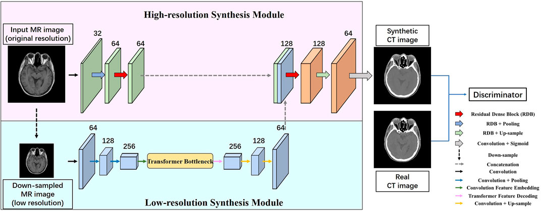
FIGURE 1. Overall structure of HMSS-Net. It contains two synthesis modules with pyramidal inputs; the low-resolution synthesis module would model down-sampled MR images whose resolution is half of that of the original images; the high-resolution synthesis module would model MR images of original resolution. These two modules have different designs to enrich the learning of local or global information. After synthesis, the synthetic CT and its corresponding real CT would be fed into the discriminator module for adversarial learning.
The low-resolution synthesis module is designed to extract global patterns in MRI–CT synthesis that could represent MRI–CT relations on widely spread tissues and large organs, thus providing a coarse anatomical background for synthetic CT. Therefore, the synthesis module should have a large receptive field to explore long-range patterns. In this module, instead of using a pure convolutional architecture whose receptive field is limited, we apply the concept of transformer to its bottleneck part. Transformer is a convolution-free model that solely relies on the attention mechanism to study contextual dependencies in the natural language processing (NLP) task, and it could analyze the correlations between every word in a sentence regardless of the distance. Vision transformer (VIT) [21] has expanded its usage to image processing with an embedding procedure to translate the image feature space to the semantic feature space and a decoding procedure as the reverse translation. Based on VIT, we build the transformer bottleneck whose detailed structure is presented in Figure 2. In addition to the bottleneck, the low-resolution synthesis module also contains a convolutional encoder and a convolutional decoder. The encoder consists of three convolutional blocks with a 3 × 3 convolutional layer, instance normalization, and Gaussian error linear unit (GELU). The average pooling layer is used between each convolution block to down-sample the feature size. The decoder consists of two convolutional blocks with the same structure as that of the encoder, and bilinear interpolation is used after each convolutional block to up-sample the feature size. In the end, the output of the low-resolution synthesis module is delivered to the high-resolution synthesis module and concatenated with the latter’s feature map.
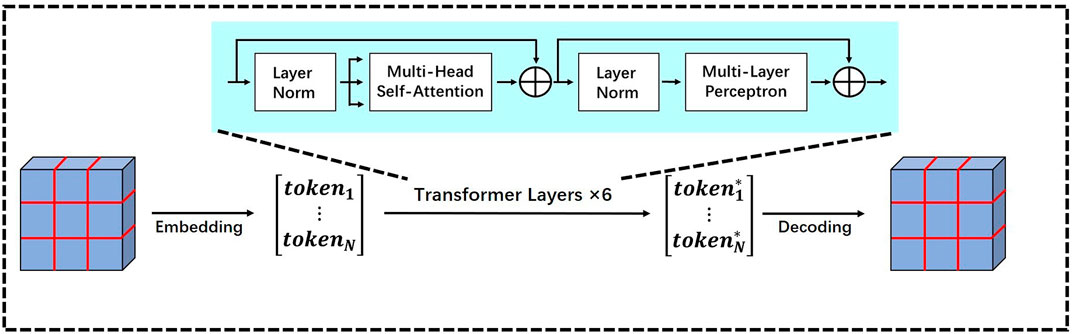
FIGURE 2. Detailed structure of the transformer bottleneck in the low-resolution synthesis module.
We provide more details of the transformer bottleneck to show how it studies the contextual correlations from its input feature map. As shown in Figure 2, it contains three procedures, i.e., embedding, transformer layer, and decoding.
Embedding: The embedding procedure aims to translate the input feature map to a sequence of semantic tokens, and each token would reflect the content information of a small patch on the original image. It contains several steps; first, the input feature map is separated into small feature patches. Then, the patches are flattened into vectors, and they further form the rows of a matrix whose height equals the number of patches and width equals the dimension of flattened patches. Given an input feature map
Transformer layer: The embedded matrix is then modeled by several transformer layers to study the contextual information. Each transformer layer is a cascaded structure of multi-head self-attention (MSA) and multi-layer perceptron (MLP). Let
where
The multi-head self-attention is a group of single-head self-attention, where each single-head self-attention independently studies the contextual correlations between every token-pair from the embedded matrix. Let
where
The relevance is further multiplied with
Such calculation could be carried out in parallel for all tokens in
where
The output of MSA is the concatenation of all single-head output, formulated as follows:
The MLP contains two fully connected layers; the first layer would double the dimension of MSA-modified tokens, and the second layer would compress the dimension back; this structure could analyze the interactions within each modified token and extract useful information.
Decoding: After modeling by the transformer layers, the output matrix
As presented in Figure 1, the convolutional encoder of the low-resolution synthesis module has 64, 128, and 256 filters in each convolutional layer. The decoder has 128 and 64 filters in each convolutional layer. In the transformer bottleneck, the input feature is separated with a patch size 3 and stride 1, and the dimension of embedded tokens
The high-resolution synthesis module is designed to explore local MRI–CT relations to synthesize detailed anatomical structures on the output of the low-resolution synthesis module. In order to enhance the learning of local structural properties, conventional convolutional blocks are replaced by residual dense blocks (RDBs), which are able to aggregate convolutional features under gradually enlarged receptive fields that could represent local patterns based on multiple step sizes.
Figure 3 presents the detailed structure of the RDB. Each block contains two densely connected 3 × 3 convolutional layers with instance normalization and GELU and an additional 1 × 1 convolutional layer to adjust the channel size to the predefined number. The dense connection would combine the features from preceding layers together with the current layer, and as 3 × 3 convolution would enlarge the receptive field by two pixels, the output would contain features under the gradually enlarged receptive field. The RDB also contains a residual connection that adds the input and output of RDB, which is designed to prevent gradient vanishing. If the input and output have different channel sizes, the input would be further modified by a 1 × 1 convolutional layer.
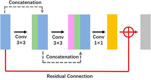
FIGURE 3. Detailed structure of the residual dense block in the high-resolution synthesis module.
The structure of the high-resolution synthesis module is given in Figure 1. It contains an encoder and a decoder. The encoder contains three blocks; the first block is a conventional convolutional block with a 3 × 3 convolutional layer, instance normalization, and GELU; the number of filters is 32; the second and third blocks are RDBs; the number of filters of each 3 × 3 convolutional layer is 16 and 32 in each RDB, respectively; their output channels are controlled to 64 and 64. The decoder contains three blocks; the first and second blocks are RDBs; the number of filters of each 3 × 3 convolutional layer is 64 and 64 in each RDB, respectively; their output channels are controlled to 128 and 64. The third block of the decoder is a convolutional block with a 1 × 1 convolutional layer to combine all channels together and a sigmoid function as non-linear activation.
As presented in Figure 1, the low-resolution synthesis module and high-resolution synthesis module are connected through feature concatenation. These modules together form the generator part of HMSS-Net. Designed as a GAN framework, HMSS-Net also contains a discriminator model to provide adversarial learning. During training, it would try to distinguish the synthetic and real CT and compete against the generator to reach the Nash equilibrium. Specifically, HMSS-Net introduced the PatchGAN discriminator from pix2pix [22]. It consists of five convolutional blocks; the first three blocks contain a convolutional layer with kernel size 4, stride size 2, and padding size 1; the rest of the blocks contain a convolutional layer with kernel size 4, stride size 1, and padding size 1. Instance normalization is used after the second, third, and fourth convolutional blocks. Consequently, an input image with shape 256 × 256 would be transformed to a 30 × 30 matrix by PatchGAN; each element of the matrix represents the discriminator’s judgement on a 70 × 70 sub-region from the input image. The number of filters of each convolutional block is 32, 64, 128, 256, and 1.
During training, the performance of synthetic CT is supervised by the loss functions; then, the results are back-propagated through HMSS-Net to update its parameters. In this study, the total loss function is a combination of L1-loss, adversarial loss, and multi-scale structural similarity index measure (MS-SSIM) loss. They could provide supervision from a different scale and different aspects. For L1-loss, it focuses on the global intensity performance of synthetic CT; for adversarial loss, it focuses on the local detailed synthesis performance; for MS-SSIM loss, it measures the similarities on three predefined aspects including luminance, contrast, and structure under five different scales [20]. Their formulas are provided as follows:
Adversarial loss: We used the LS-GAN method [23] to calculate the adversarial loss. Let
where
where
L1-loss: L1-loss is a direct way to evaluate the intensity difference between the synthetic and real CT, and its definition is as follows:
where N is the total number of elements in synthetic or real CT.
MS-SSIM Loss: SSIM is a widely used metric to evaluate the similarity between two images. Compared with the mean absolute error (MAE) or mean squared error (MSE), SSIM is more comprehensive as it combines the similarities of luminance, contrast, and structure. These similarities are quantified by the mean value, standard deviation, and co-variance on image patches with step size
where
Then, the SSIM of the patch is defined by multiplying
Finally, the SSIM between synthetic and real CT images is defined as the mean value of all patches.
Typically, SSIM uses a
where
Finally, the MS-SSIM loss is defined as follows:
Total Loss: The total loss function is the weighted summary of the aforementioned loss functions, given by
where
To provide quantitative evaluations to the performance of synthetic CT, this study introduced five kinds of metrics, namely, the mean absolute error (MAE), peak signal-to-noise ratio (PSNR), dice similarity coefficient of bone (Bone_DSC), SSIM, and MS-SSIM. The metrics could judge the performance of synthetic CT from multiple angles. The meaning and definition of SSIM and MS-SSIM have been given in the aforementioned section. The MAE and PSNR mainly focus on the intensity performance of synthetic CT. The Bone_DSC evaluates the structural performance using bone as the representative. Their definitions are given as follows:
where N is the number of valid pixels on the head and neck regions; MAX is the maximum intensity value of real CT;
Before training, the MR and CT images were preprocessed with several steps. First, each slice was resampled to the spatial resolution of 1 × 1 mm2; then, the unnecessary background region was cropped to unify the size to 256 × 256 for the deep network input. Each patient’s MRI was aligned rigidly to the corresponding CT under 3D registration by the ‘ANTs’ package [24]. N4BiasFieldCorrection [25] and histogram matching [26] procedures were also applied to MR images to correct the intensity inhomogeneity and reduce the intensity variance among different patients. Finally, the maximum values of MR and CT images were cut off to 800 and 1400 HU, respectively, and the images were then scaled to [0, 1].
The 78 patients were randomly sampled into three datasets for training, validation, and test by 80%, 10%, and 10%, respectively, and the corresponding numbers were 62, 8, and 8. During training, the network parameters that yielded the best performance on the validation set were saved and used to evaluate the performance on the test set. Before training, the data augmentation method was applied to the training set to increase the robustness of the model, which contained random shift, flip, and rotation.
The proposed study was implemented using PyTorch 1.7.1 on the Python 3.8 platform by a NVIDIA GeForce GTX 1080 Ti GPU that contains 11 GB memory. The hyperparameters of the network were listed as follows: the maximum training epoch was 120, the batch size was set to be 3, the Adam optimizer was set to use with β_1 = 0.5 and β_2 = 0.9, and the initial learning rate was 10–4. The learning rate was automatically controlled by a method called ‘ReduceLROnPlateau’, when the performance of the validation set did not improve within 10 epochs, and the learning rate would decay by 30%.
In order to evaluate the performance of HMSS-Net, we conducted several comparative studies between it and two state-of-the-art methods. The first method is the pix2pixHD that has shown its effectiveness on MRI–CT synthesis in the work of Boni et al. [15]. As an improved version of pix2pix, pix2pixHD is designed as a coarse-to-fine model that enables the multi-scale learning, which is purely built on convolution-based models. The second method is the PTNet that was proposed for cross-MRI synthesis in the work of Zhang et al [16]. It is also a multi-scale learning framework but is purely based on the Transformer method. Compared with them, HMSS-Net is a hybrid structure with convolution- and transformer-based designs targeting at the learning of local and global MRI–CT relations, respectively.
Table 1 summarizes the quantitative evaluations on the performance of synthetic CT by HMSS-Net, pix2pixHD, and PTNet in the test set. Numerical results are displayed by the mean (±standard deviation). The two-tailed paired t-test between HMSS-Net and other models on each evaluation metric was applied to analyze the significances of the results, and corresponding p-values are also displayed in Table 1. It is evident that HMSS-Net achieved the best performances on all metrics, as it reduced the mean MAE of 7.6/3.13 HU, increased the mean PSNR of 1.41/0.97 dB, increased the mean Bone_DSC of 0.021/0.018, increased the mean SSIM of 0.031/0.006, and increased the mean MS-SSIM of 0.038/0.016 compared with pix2pixHD/PTNet. Moreover, these improvements were all statistically significant with p-value < 0.05.
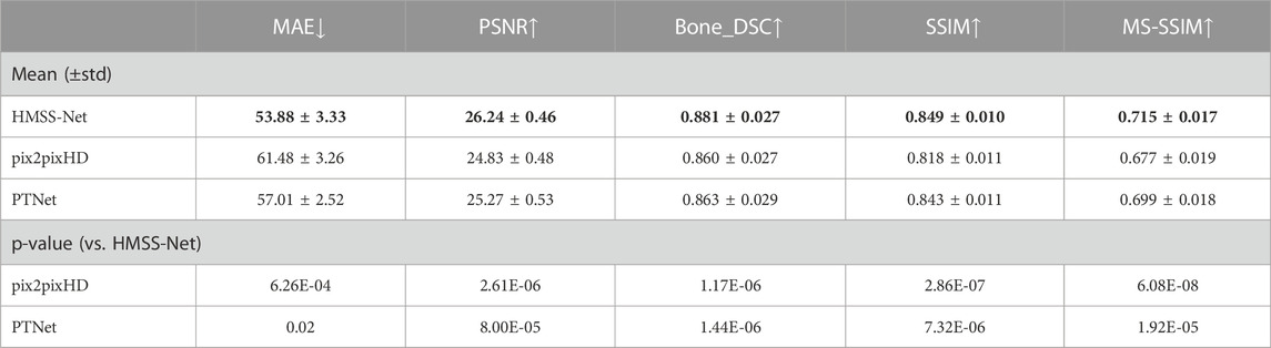
TABLE 1. Quantitative evaluations of HMSS-Net, pix2pixHD, and PTNet. The down arrow means that the lower number of this metric indicates better performance; the up arrow means that higher number of this metric indicates better performance.
We also provided qualitative evaluations of HMSS-Net, pix2pixHD, and PTNet. Figure 4 presents two slices of synthetic CT by pix2pixHD (a1 and a5), PTNet (a2 and a6), HMSS-Net (a3 and a7), and the corresponding real CT (a4 and a8) which is labeled as the ‘ground truth.’ To present the difference between synthetic and real CT, difference maps under two display windows are also given in Figure 4, where one ranges from -100 HU to 100 HU to highlight the soft-tissue difference and the other ranges from -1000 HU to 1000 HU to highlight the bone difference. The display windows are shown in (b4 and b8) and (c4 and c8). The difference maps are placed in (b1, b5, c1, and c5) for pix2pixHD, (b2, b6, c2, and c6) for PTNet, and (b3, b7, c3, and c7) for HMSS-Net. It is evident that all difference maps of HMSS-Net have lighter color than those of pix2pixHD and PTNet, which means that HMSS-Net provided more accurate synthetic results on the intensity of both tissues. In addition, the difference map (c3) of HMSS-Net has a thinner deep region around the skull than (c1 and c2), while (c7) has a smaller deep region around the spine than (c5 and c6). This finding could suggest that HMSS-Net reduced the structural differences on tissue boundaries.
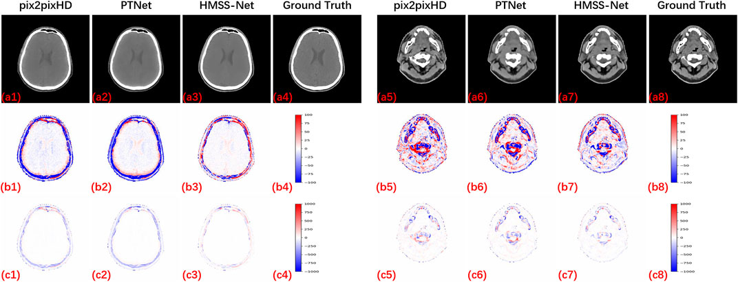
FIGURE 4. Synthetic results of pix2pixHD, PTNet, and HMSS-Net with two kinds of difference maps for qualitative comparison. All CT images are displayed with a soft-tissue window [-125, 225] HU to provide a clear visualization of the tissues.
Figure 5 presents the zoomed-in CT regions to evaluate the local synthetic performance. (a1 and a5), (a2 and a6), and (a3 and a7) are two slices of synthetic CT by pix2pixHD, PTNet, and HMSS-Net, respectively, and (a4 and a8) are the corresponding real CT. (b1∼b8) are the zoomed-in regions in the red box on (a1∼a8). The first slice is in a layer containing the eyeball; we could see that pix2pixHD and PTNet did not provide a smooth bone structure pointed by the green arrows in (b1 and b2). The second slice is in a layer containing the nasal cavity, pix2pixHD, and PTNet-synthesized discontinuous bone structure pointed by the green arrows in (b5 and b6), whereas HMSS-Net provided good synthetic performances shown in (b3 and b7), illustrating its ability to provide more accurate detailed structures.
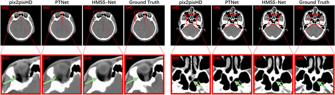
FIGURE 5. Results of pix2pixHD, PTNet, HMSS-Net, and the corresponding real CT with the zoomed-in detailed structure for qualitative comparison.
From the quantitative and qualitative evaluations, we could find their accordance to demonstrate the ability of HMSS-Net on MRI–CT synthesis. This implies that HMSS-Net is able to enhance the learning of local and global MRI–CT relations and utilize them to improve the intensity and structural performances of synthetic CT.
HMSS-Net is designed to enhance the learning and utilization of multi-scale information through the following parts: 1) the transformer bottleneck in the low-resolution synthesis module which enables the learning of global contextual correlations; 2) the RDB in the high-resolution synthesis module which could combine the local patterns under different step sizes; and 3) the MS-SSIM loss which could provide multi-scale supervision. To verify the contribution of each part to the performance of synthetic CT, we conducted three ablation studies: 1) replacing the transformer bottleneck by the conventional convolutional bottleneck, which is denoted as ‘w/o TB’; 2) replacing each RDB by a conventional convolutional block, which is denoted as ‘w/o RDB’; and 3) removing the MS-SSIM loss during training, which is denoted as ‘w/o MS-SSIM.’
Table 2 presents the quantitative evaluations of the ablation studies with HMSS-Net. First, when the transformer bottleneck is replaced, the mean MAE is increased by 2.25 HU, PSNR is decreased by 0.81 dB, Bone_DSC is decreased by 0.007, SSIM is decreased by 0.011, and MS-SSIM is decreased by 0.031. The sharp reduction on the performance of synthetic CT could demonstrate the importance of the transformer bottleneck in HMSS-Net, and it also implies that the transformer bottleneck is better at learning global MRI–CT relations than conventional convolution blocks. Second, when the RDB is replaced, the mean MAE is increased by 0.73 HU, PSNR is decreased by 0.28 dB, Bone_DSC is decreased by 0.007, SSIM is decreased by 0.009, and MS-SSIM is decreased by 0.017. These numbers indicate that RDB is also important to HMSS-Net for enriching local MRI–CT relations. Moreover, as RDB focuses more on the local patterns, its influence on the global intensity performance might be less than that of the transformer bottleneck, which could be inferred from the comparisons on MAE and PSNR. Finally, when training without the MS-SSIM loss, the mean MAE is increased by 0.57 HU, PSNR is decreased by 0.06 dB, Bone_DSC is decreased to 0.003, SSIM is decreased by 0.003, and MS-SSIM is decreased by 0.007. The changes on metrics are small compared with those of other ablation studies; however, the use of MS-SSIM loss still has a positive influence on the overall performance of synthetic CT.
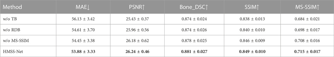
TABLE 2. Quantitative evaluations of the ablation studies and HMSS-Net.
In this study, we proposed a new MRI–CT synthesis model with a multi-scale learning framework. Before our study, some multi-scale-based studies used similar network architectures to model different scales of an input image, including a pure convolution-based model like pix2pixHD and a pure transformer-based model like PTNet. Different from them, the proposed HMSS-Net is a hybrid model with proper designs to take advantage of both methods and fully exploit local and global MRI–CT relations. In the comparisons between HMSS-Net with pix2pixHD and PTNet, we showed that our method could significantly improve the intensity and structural performance of synthetic CT. We also demonstrated the contribution of each method through ablation studies. Alongside the framework, we introduced the MS-SSIM loss to MRI–CT synthesis to provide multi-scale supervision, and the experimental results have proven its contribution to the performance of synthetic CT.
An important finding in our study is the dice of the bone between synthetic and real CT. In current studies, the synthesis of the bone structure is one of the most challenging parts, not only because bone has complex structures but also because its signal on conventional MRI sequences is very low, which makes it hard to be distinguished with air. Meanwhile, accurately synthesizing its structure has great clinical significance because bone could easily absorb X-rays. According to existing MRI–CT synthesis studies, the dice between synthetic and real CT was not very satisfying, even though the authors have introduced techniques to enrich its pattern learning. For example, the work of Haley et al. achieved 0.764 under an Inception V3-based convolutional network; the work of Yang et al. [27] achieved 0.83 under a densely connected convolutional network; the work of Dinkla et al. [14] achieved 0.85 under a dilated convolution-based network. Compared with them, the proposed HMSS-Net showed a stronger ability to study the property of bone and translate it from MRI to CT by increasing the dice to 0.883. Therefore, our method is competing on bone synthesis and has significant potential for clinical usage.
As our experiment was based on clinical data, a small portion of the set contains artifacts that influence the original MR or CT image. In Figure 6, we presented the CT and MR images of a patient from the test set who had dental filling issues, and the severe artifact around the filling region is clearly observed on the CT image. We could find that our method was not sensitive to this situation; it treated the input MR image the same way as normal data and provided synthetic CT with the artifact being ‘corrected’. The main reason might be that only three of 62 patients in the training set have this issue, and it only affects 1–2 slices in each patient, which is not sufficient to train a deep learning model. As shown in the difference map, the artifact region has a larger intensity difference between synthetic and real CT, which lowers the calculation numbers. In addition, it is hard to say whether the ‘corrected’ result is more useful in the clinic because it might mis-inform doctors about the actual dental condition. In further study, we hope to design a more proper approach to deal with data with the artifact and provide two versions of synthetic CT so that one keeps the artifact and one automatically removes the artifact for different usage.
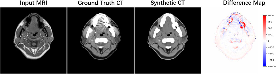
FIGURE 6. Example of data with the dental artifact. The patient’s real MRI, real CT, and synthetic CT by HMSS-Net and the difference map under the [-1,000, 1,000] display window are provided from the left column to the right column.
Although HMSS-Net has achieved considerable results, it still has some limitations. This model uses a single MRI sequence to synthesize CT, which should be extended to multi-MRI sequences because more MRI sequences could bring more structural information to enrich MRI–CT relations [11]. In addition, HMSS-Net uses paired MRI and CT data for training, which introduces the MRI–CT registration error. To solve this problem, it could be designed to the CycleGAN framework [28] which could train unpaired data. Finally, HMSS-Net could benefit from 3D networks to preserve vertical continuity, but we need larger GPU memory for whole 3D inputs with the consideration that a 3D image patch like 32 × 32×32 [6] makes no sense to the learning of global contextual information in the transformer bottleneck.
We propose a hybrid multi-scale model for MRI–CT synthesis, which enhances the learning of local MRI–CT relations with residual and dense connections and the learning of global MRI–CT relations with the transformer bottleneck. In addition to the network structure, the proposed HMSS-Net is supervised by MS-SSIM loss that enables multi-scale supervision. The comprehensive evaluations show the ability of HMSS-Net on providing accurate intensity and structural performances of synthetic CT. HMSS-Net, therefore, has the potential for clinical applications.
The original contributions presented in the study are included in the article/Supplementary Material; further inquiries can be directed to the corresponding authors.
The studies involving human participants were reviewed and approved by the Institutional Review Boards committee of Sun Yat-sen University Cancer Center, with the approval number GZKJ2020-008. The patients/participants provided their written informed consent to participate in this study.
Investigation, YLi, SX, and ZQ; methodology, YLi; resources, ZQ and SX; writing—original draft preparation, YLi and SX; writing—review and editing, YLu and ZQ. All authors have read and agreed to the published version of the manuscript.
This work was funded in part by the NSFC under Grant 12126610, Grant 81971691, Grant 81801809, Grant 81830052, Grant 81827802, and Grant U1811461; in part by the Science and Technology Program of Guangzhou under Grant 201804020053; in part by the Science and Technology Innovative Project of Guangdong Province under Grant 2018B030312002; in part by the Department of Science and Technology of Jilin Province under Grant 20190302108GX; in part by the Construction Project of the Shanghai Key Laboratory of Molecular Imaging under Grant 18DZ2260400; in part by the Guangdong Province Key Laboratory of Computational Science at the Sun Yat-sen University under Grant 2020B1212060032; in part by the Key-Area Research and Development Program of Guangdong Province under Grant 2021B0101190003; and in part by the Science and Technology Program of Guangzhou under Grant 202206010180.
The authors declare that the research was conducted in the absence of any commercial or financial relationships that could be construed as a potential conflict of interest.
All claims expressed in this article are solely those of the authors and do not necessarily represent those of their affiliated organizations, or those of the publisher, the editors, and the reviewers. Any product that may be evaluated in this article, or claim that may be made by its manufacturer, is not guaranteed or endorsed by the publisher.
1. Chandarana H, Wang H, Tijssen R, Das IJ. Emerging role of MRI in radiation therapy. J Magn Reson Imaging (2018) 48(6):1468–78. doi:10.1002/jmri.26271
2. Schneider W, Bortfeld T, Schlegel W. Correlation between CT numbers and tissue parameters needed for Monte Carlo simulations of clinical dose distributions. Phys Med Biol (2000) 45(2):459–78. doi:10.1088/0031-9155/45/2/314
3. Edmund JM, Nyholm T. A review of substitute CT generation for MRI-only radiation therapy. Radiat Oncol (2017) 12(1):28. doi:10.1186/s13014-016-0747-y
4. LeCun Y, Bengio Y, Hinton G. Deep learning. Nature (2015) 521(7553):436–44. doi:10.1038/nature14539
5. Han X. MR-based synthetic CT generation using a deep convolutional neural network method. Med Phys (2017) 44(4):1408–19. doi:10.1002/mp.12155
6. Nie D, Trullo R, Lian J, Wang L, Petitjean C, Ruan S, et al. Medical image synthesis with deep convolutional adversarial networks. IEEE Trans Biomed Eng (2018) 65(12):2720–30. doi:10.1109/TBME.2018.2814538
7. Maspero M, Savenije MHF, Dinkla AM, Seevinck PR, Intven MPW, Jurgenliemk-Schulz IM, et al. Dose evaluation of fast synthetic-CT generation using a generative adversarial network for general pelvis MR-only radiotherapy. Phys Med Biol (2018) 63(18):185001. doi:10.1088/1361-6560/aada6d
8. Wolterink JM, Dinkla AM, Savenije MHF, Seevinck PR, van den Berg CAT, Išgum I. Deep MR to CT synthesis using unpaired data. In: Tsaftaris SA, Gooya A, Frangi AF, Prince JL, editors. Simulation and synthesis in medical imaging. Cham: Springer International Publishing (2017). p. 14–23.
9. Yang H, Sun J, Carass A, Zhao C, Lee J, Prince JL, et al. Unsupervised MR-to-CT synthesis using structure-constrained CycleGAN. IEEE Trans Med Imaging (2020) 39(12):4249–61. doi:10.1109/TMI.2020.3015379
10. Tie X, Lam SK, Zhang Y, Lee KH, Au KH, Cai J. Pseudo-CT generation from multi-parametric MRI using a novel multi-channel multi-path conditional generative adversarial network for nasopharyngeal carcinoma patients. Med Phys (2020) 47(4):1750–62. doi:10.1002/mp.14062
11. Qi M, Li Y, Wu A, Jia Q, Li B, Sun W, et al. Multi-sequence MR image-based synthetic CT generation using a generative adversarial network for head and neck MRI-only radiotherapy. Med Phys (2020) 47(4):1880–94. doi:10.1002/mp.14075
12. Massa HA, Johnson JM, McMillan AB. Comparison of deep learning synthesis of synthetic CTs using clinical MRI inputs. Phys Med Biol (2020) 65(23):23NT03. doi:10.1088/1361-6560/abc5cb
13. Szegedy C, Vanhoucke V, Ioffe S, Shlens J, Wojna Z. Rethinking the inception architecture for computer vision. In: presented at the Proceedings of the IEEE conference on computer vision and pattern recognition; June 2016; Las Vegas, NV, USA. IEEE (2016).
14. Dinkla AM, Wolterink JM, Maspero M, Savenije MH, Verhoeff JJ, Seravalli E, et al. MR-only brain radiation therapy: Dosimetric evaluation of synthetic CTs generated by a dilated convolutional neural network. Int J Radiat Oncol Biol Phys (2018) 102(4):801–12. doi:10.1016/j.ijrobp.2018.05.058
15. Boni KNDB, Klein J, Vanquin L, Wagner A, Lacornerie T, Pasquier D, et al. MR to CT synthesis with multicenter data in the pelvic area using a conditional generative adversarial network. Phys Med Biol (2020) 65(7):075002. doi:10.1088/1361-6560/ab7633
16. Zhang X, He X, Guo J, Ettehadi N, Aw N, Semanek D, et al. Ptnet: A high-resolution infant MRI synthesizer based on transformer (2021). arXiv preprint arXiv:2105.13993.
17. Chen J, Lu Y, Yu Q, Luo X, Adeli E, Wang Y, et al. Transunet: Transformers make strong encoders for medical image segmentation (2021). arXiv preprint arXiv:2102.04306.
18. Vaswani A, Shazeer N, Parmar N, Uszkoreit J, Jones L, Gomez AN, et al. Attention is all you need. Adv Neural Inf Process Syst (2017) 30. doi:10.48550/arXiv.1706.03762
19. Zhang Y, Tian Y, Kong Y, Zhong B, Fu Y. Residual dense network for image super-resolution. In: presented at the Proceedings of the IEEE conference on computer vision and pattern recognition; June 2018. IEEE (2018). p. 2472–81.
20. Zhao H, Gallo O, Frosio I, Kautz J. Loss functions for image restoration with neural networks. IEEE Trans Comput Imaging (2017) 3(1):47–57. doi:10.1109/tci.2016.2644865
21. Dosovitskiy A, Beyer L, Kolesnikov A, Weissenborn D, Zhai X, Unterthiner T, et al. An image is worth 16x16 words: Transformers for image recognition at scale (2020). arXiv preprint arXiv:2010.11929.
22. Isola P, Zhu J, Zhou T, Efros AA. Image-to-image translation with conditional adversarial networks. In: presented at the Proceedings of the IEEE conference on computer vision and pattern recognition; July 2017. IEEE (2017).
23. Mao X, Li Q, Xie H, Lau RY, Wang Z, Paul Smolley S. Least squares generative adversarial networks. In: presented at the Proceedings of the IEEE international conference on computer vision; October 2017. IEEE (2017).
24. Avants BB, Tustison N, Song G. Advanced normalization tools (ANTS). Insight J (2009) 2(365):1–35. doi:10.54294/uvnhin
25. Tustison NJ, Avants BB, Cook PA, Zheng Y, Egan A, Yushkevich PA, et al. N4ITK: Improved N3 bias correction. IEEE T Med Imaging (2010) 29(6):1310–20. doi:10.1109/tmi.2010.2046908
26. Nyul LG, Udupa JK, Zhang X. New variants of a method of MRI scale standardization. IEEE Trans Med Imaging (2000) 19(2):143–50. doi:10.1109/42.836373
27. Lei Y, Harms J, Wang T, Liu Y, Shu H, Jani AB, et al. MRI-only based synthetic CT generation using dense cycle consistent generative adversarial networks. Med Phys (2019) 46(8):3565–81. doi:10.1002/mp.13617
Keywords: MRI–CT synthesis, multi-scale learning, deep learning, transformer, hybrid model, convolution
Citation: Li Y, Xu S, Lu Y and Qi Z (2023) CT synthesis from MRI with an improved multi-scale learning network. Front. Phys. 11:1088899. doi: 10.3389/fphy.2023.1088899
Received: 03 November 2022; Accepted: 06 January 2023;
Published: 23 January 2023.
Edited by:
Junxin Chen, Dalian University of Technology, ChinaReviewed by:
Hao Gao, Nanjing University of Posts and Telecommunications, ChinaCopyright © 2023 Li, Xu, Lu and Qi. This is an open-access article distributed under the terms of the Creative Commons Attribution License (CC BY). The use, distribution or reproduction in other forums is permitted, provided the original author(s) and the copyright owner(s) are credited and that the original publication in this journal is cited, in accordance with accepted academic practice. No use, distribution or reproduction is permitted which does not comply with these terms.
*Correspondence: Zhenyu Qi, cWl6aHlAc3lzdWNjLm9yZy5jbg==; Yao Lu, bHV5YW8yM0BtYWlsLnN5c3UuZWR1LmNu
†These authors have contributed equally to this work and share first authorship
Disclaimer: All claims expressed in this article are solely those of the authors and do not necessarily represent those of their affiliated organizations, or those of the publisher, the editors and the reviewers. Any product that may be evaluated in this article or claim that may be made by its manufacturer is not guaranteed or endorsed by the publisher.
Research integrity at Frontiers
Learn more about the work of our research integrity team to safeguard the quality of each article we publish.