
94% of researchers rate our articles as excellent or good
Learn more about the work of our research integrity team to safeguard the quality of each article we publish.
Find out more
ORIGINAL RESEARCH article
Front. Phys., 26 June 2023
Sec. Statistical and Computational Physics
Volume 11 - 2023 | https://doi.org/10.3389/fphy.2023.1061580
This article is part of the Research TopicHeterogeneous Computing in Physics-Based ModelsView all 5 articles
In this study, we explore the similarities and differences between variational Monte Carlo techniques that employ conventional and artificial neural network representations of the ground-state wave function for fermionic systems. Our primary focus is on shallow neural network architectures, specifically the restricted Boltzmann machine, and we examine unsupervised learning algorithms that are appropriate for modeling complex many-body correlations. We assess the advantages and drawbacks of conventional and neural network wave functions by applying them to a range of circular quantum dot systems. Our findings, which include results for systems containing up to 90 electrons, emphasize the efficient implementation of these methods on both homogeneous and heterogeneous high-performance computing facilities.
Solving the Schrödinger equation for systems of many interacting bosons or fermions is classified as an NP-hard problem due to the complexity of the required many-dimensional wave function, resulting in an exponential growth of degrees of freedom. Reducing the dimensionalities of quantum mechanical many-body systems is an important aspect of modern physics, ranging from the development of efficient algorithms for studying many-body systems to exploiting the increase in computing power. To write software that can fully utilize the available resources has long been known to be an important aspect of these endeavors. Despite tremendous progress having been made in this direction, traditional many-particle methods, either quantum mechanical or classical ones, face huge dimensionality problems when applied to studies of systems with many interacting particles.
Over the last 2 decades, quantum computing and machine learning have emerged as some of the most promising approaches for studying complex physical systems where several length and energy scales are involved. Machine learning techniques and in particular neural-network quantum states Goodfellow et al. [1] have recently been applied to studies of many-body systems, see, for example, Refs. Carleo and Troyer [2]; Carrasquilla and Torlai [3]; Pfau et al. [4]; Calcavecchia et al. [5]; Carleo et al. [6]; Boehnlein et al. [7]; Adams et al. [8]; Lovato et al. [9], in various fields of physics and quantum chemistry, with very promising results. In many of these studies, results have aligned well with exact analytical solutions or are in close agreement with state-of-the-art quantum Monte Carlo calculations.
The variational and diffusion Monte Carlo algorithms are among the most popular and successful methods available for ground-state studies of quantum mechanical systems. They both rely on a suitable ansatz for the ground-state of the system, often dubbed the trial wave function, which is defined in terms of a set of variational parameters whose optimal values are found by minimizing the total energy of the system. Devising flexible and accurate functional forms for the trial wave functions requires prior knowledge and physical intuition about the system under investigation. However, for many systems we do not have this intuition, and as a result it is often difficult to define a good ansatz for the state function.
According to the universal approximation theorem, a deep feedforward neural network can represent any continuous function within a certain error Hornik et al. [10] — see also Refs. Murphy [11]; Hastie et al. [12]; Bishop [13]; Goodfellow et al. [1] for further discussions of deep learning methods. Since the variational state in principle can take any functional form, it is natural to replace the trial wave function with a neural network and treat it as a machine learning problem. This approach has been successfully implemented in recent works, see, for example, Refs. Pfau et al. [4]; Carleo and Troyer [2]; Cassella et al. [14]; Adams et al. [8]; Lovato et al. [9], and forms the motivation for the present study. Here, the neural network of choice was derived from so-called Gaussian-binary restricted Boltzmann machines, much inspired by the recent contributions by Carleo et al., see, for example, Refs. Carleo and Troyer [2]; Carleo et al. [6]. Unlike binary-binary restricted Boltzmann machines Sieber and Gehringer [15], the approximation properties of Gaussian-binary restricted Boltzmann aren’t yet well-understood. However, they are considered highly-expressive networks for certain problems, such as dimensionality reduction and continuous probability density estimation. Note that neural-network representations of variational states are more general, as they don’t in principle require prior knowledge of the ground-state wave function, thereby opening the door to systems that have yet to be solved. Particular attention however has to be devoted to the symmetries of the problem, whose inclusion is critical to achieve accurate results.
In this work, we will focus on systems of electrons confined to move in two-dimensional harmonic oscillator systems, so-called quantum dots. These are strongly confined electrons and offer a wide variety of complex and subtle phenomena which pose severe challenges to existing many-body methods. Due to their small size, quantum dots are characterized by discrete quantum levels. For instance, the ground states of circular dots show similar shell structures and magic numbers as seen for atoms and nuclei. These structures are particularly evident in measurements of the change in electrochemical potential due to the addition of one extra electron. Here, these systems will serve as our test of the applicability of restricted Boltzmann machines as artificial neural network variational states.
The theoretical foundation and the methodology are explained in Section 2. The subsequent sections present our results with an analysis of computational methods and resources. In the last section we present our conclusions and perspectives for future work.
For any Hamiltonian
Thus, approximate solutions to the time-independent Schrödinger equation can be obtained by choosing a careful parameterization of the wave function and minimizing the energy ET with respect to the parameters. Since the integrals representing ET are normally high dimensional, it is most efficient to evaluate them by means of Monte Carlo methods
This involves collecting n samples of configurations and averaging over the so-called local energies
We apply the variational Monte Carlo (VMC) method to various circular quantum dots systems. These are systems of interacting electrons confined to move in a two-dimensional harmonic oscillator well. The (scaled)1 Hamiltonian is given by
where ω is the oscillator frequency, ri is the distance between electron i and the origin, and rij is the distance between electrons i and j. We will henceforth assume the total number of electrons N to be even and the total spin of the system to be zero.
A simple ansatz can be built starting from the analytical solutions to the non-interacting case. The harmonic oscillator eigenfunctions are given by
where Hn are the Hermite polynomials of degree n. To constrain the antisymmetry of the many-body wave function, products of the lowest N/2 spatial states and the two spin states ξ±(σ) are used as a basis for a Slater determinant
where m, n, k label the single-particle state, i labels the particle, and R contains all coordinates of the N particles. As an aside, we do not include the spin projections σi as explicit inputs to the wave function as we will describe how to treat them separately in Section 2.2. We then define a reference state by pulling the common exponential term out of the determinant and inserting a single variational parameter α
Correlations among electrons can be handled by a Padé-Jastrow factor Drummond et al. [16],
where β is a variational parameter and
in order for the Kato cusp condition to be satisfied Huang et al. [17]. The product of the Slater determinant and the Padé-Jastrow factor is commonly named the Slater-Jastrow ansatz,
There are many possible choices for a machine learning inspired wave function, but using an artificial neural network has recently been demonstrated to give remarkably good results in studies of quantum mechanical many-body systems Cassella et al. [14]; Adams et al. [8]; Lovato et al. [9]; Fore et al. [18]; Rigo et al. [19]. Inspired by Ref. Carleo and Troyer [2], our choice is to start from a restricted Boltzmann machine (RBM) configured for continuous inputs, illustrated in Figure 1. The inputs
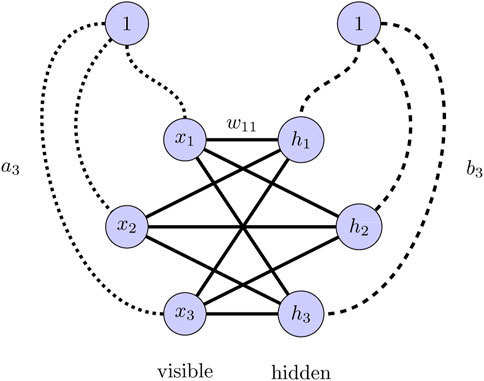
FIGURE 1. Architecture of a restricted Boltzmann machine. Inter-layer connections between the visible and the hidden layer are represented by the solid lines, where, for instance, the line connecting x1 to h1 represents the weight w11. The dotted lines represent the visible biases, where the line going from the bias unit to the visible unit x3 represents the bias weight a3. The dashed lines represent the hidden biases, where the line going from the bias unit to the hidden unit h3 represents the bias weight b3.
Here,
Notice how the marginal distribution in Eq. 9 mimics the Gaussian parts of our aforementioned ansatzes in Eqs 6, 8. Based on such observations, our next step is to construct two corresponding ansatzes
and
The two trial wave functions above apply different levels of physical intuition. While ψRBM doesn’t contain specific information about the electron-electron interactions, ψRBM+PJ contains a correlation factor that explicitly upholds the cusp condition. Both ansatzes contain knowledge about the required antisymmetry and the Gaussians in the marginal distribution help localize the wave functions to satisfy the boundary conditions far from the oscillator well. Also, as the marginal distribution is positive definite, these ansatzes will never collapse into the bosonic state even if the marginal distribution is not symmetric.
Parallel computing is an important part of our efforts for developing an efficient VMC solver. However, increasing the available computational resources alone is often not sufficient. One should also consider developing sophisticated algorithms that deliberately minimize the number of floating point operations, cache misses, and communication between parallel processes. Reducing the number of floating point operations is important in Monte Carlo calculations, in particular for the calculations reported here where we produce a large quantity (typically close to a billion) of samples. To see this, one can consider the evaluation of the kinetic energy. The kinetic energy term of the Schrödinger equation is usually one of the more computationally expensive parts to compute in terms of computing cycles. It includes, amongst other elements, the computation of the Laplacian of the wave function. The Laplacian term in the expression for the local energy can be written as
This way of writing the kinetic energy term is beneficial for two reasons: First, our trial wave function has normally an exponential shape, which is taken care of by the log-function. This is often the case for many other ansatzes for the trial functions. Secondly, this form allows for separating various elements of the trial wave function and reducing thereby the number of floating point operations. Evaluating the left-hand side of the above equation directly as it stands requires more floating point operations than evaluating the first and second derivatives of the logaritmic function. Moreover, with a logarithmic function and exponential functions as ansatzes for the trial wave function, this facilitates the use of automatic differentiation Neidinger [20]; Baydin et al. [21].
By writing the trial wave function as a product of various terms, here ψT = ∏jψj, the kinetic energy terms from each particle i can be written as a sum of their corresponding Laplacians and gradients
Obtaining analytical expressions of the gradient and Laplacian for all the wave function elements is usually computationally advantageous. However, in many Monte Carlo studies they are normally evaluated numerically using automatic differentiation Neidinger [20]; Baydin et al. [21]. Nowadays, automatic differentiation algorithms are employed routinely in VMC calculations.
The computational complexity of calculating the determinant in the näive way is proportional to
The gradient and Laplacian of the logarithm of a determinant with respect to particle i are given by
where dji is element (j, i) of the matrix and
such that the new inverse Slater matrix can be found by a few operations when the previous is known. Here, Ri is the ratio between the new and the old determinant and Sij is the cross product between columns in the new rows and the old matrix,
By using these expressions, the entire Slater determinant matrix is inverted only once per simulation. We also avoid including spin flips in the simulations. We limit ourselves in this work to systems where we can use these approximations. For systems where all single-particle states up to the Fermi level are filled, the above serves as a useful approximation if the Hamiltonian does not contain spin-dependent terms. If not, every suggested move should include possible spin flips as well.
Like most other Monte Carlo schemes, the algorithm can be split into smaller individual parts and run efficiently in parallel. For each optimization step, the system is sampled independently in several processes, and the results from all the processes are averaged before performing the parameter optimization. In this way, we achieve near perfect parallelization with message passing interface (MPI). A flow chart of the simulation code can be found in Figure 2. Notice that the parameters are updated with respect to the gradients of the expectation value of the local energy. The latter is given by
as discussed by Ref. Umrigar and Filippi [23], among others. When the simulations are run with a burn-in period2, each process should have a burn-in time equal to the burn-in time for a single process. The theoretical parallelization efficiency is then given by (tburn-in + tsample)/(mtburn-in + tsample) where m is the number of parallel processes, tburn-in is the burn-in time and tsample is the total sampling time. Additionally, the weight optimization can’t be parallelized, but has a negligible computational cost compared to the sampling. The communication can also be neglected even with low communication speed. The type of Markov-chain Monte Carlo simulations discussed here are rather simple to parallelize with almost no cost from communication between processes.
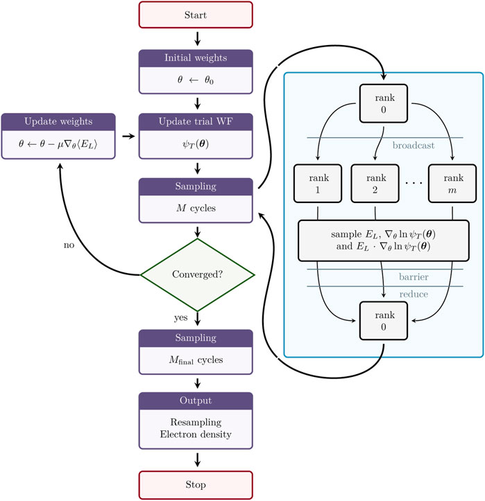
FIGURE 2. Flow chart of the solver with emphasis on the parallel processing. The sampling is parallelized across m processes, where the trial wave function (WF) is broadcast from process 0. Then EL, ∇θ ln ψT and EL ⋅∇θ ln ψT are sampled independently on each process, and an average is taken after all processes are done with sampling.
In this section we compare the computational complexity, ground state energy, energy convergence, contribution from the different Hamiltonian terms and electron densities for various trial wave function ansatzes. The RBM ansatz consists of a Slater determinant with Hermite polynomials as the basis, multiplied with the RBM marginal distribution, as presented in Eq. 10 We have not made any attempt to include optimized single-particle state functions through mean-field optimizations like Hartree-Fock theory. The second ansatz is the RBM ansatz with a correlation factor described in Eq. 7, abbreviated RBM + PJ. We have also include results obtained using a traditional Slater-Jastrow ansatz (Eq. 8), and as reference we use a plain Slater determinant (without a correlation factor, Eq. 6). The diffusion Monte Carlo (DMC) results obtained by Høgberget [24] are our main reference for the ground state energy. For quantum dots with two electrons we compare our results with corresponding analytical ones from Ref. Taut [25].
Figure 3 displays the average CPU time per iteration as a function of system size for the different wave function ansatzes. To obtain these estimates, we averaged the CPU time per iteration over 103 iterations. The RBM + PJ and Slater-Jastrow ansatzes are the most computationally demanding due to the Padé-Jastrow factor, which depends on the relative distance between electrons and requires updating of a matrix containing electron-electron distances. Each process has its own memory, and the matrix is not shared across processes.
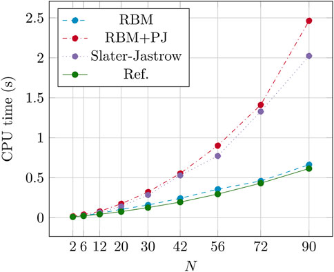
FIGURE 3. CPU time per iteration as a function of the number of electron N in a quantum dot well. Here we have employed 104 Monte Carlo cycles per iteration (with 103 iterations in total to reach an acceptable statistical error). The number of hidden nodes in the Boltzmann machine was set to H = 6.
The impact of parallel processing on computational overhead is minimal compared to other aspects of the code, except for the burn-in period. In fact, the variation in CPU time as a result of noise is much more important than the variation due to parallel processing. Additional information on CPU time per iteration for different wave function ansatzes is presented in Table 1. The reported calculations were performed for 104 Monte Carlo cycles and an oscillator frequency of ω = 1.0, with similar results for other values of ω. Each benchmark simulation was run on a single core without a burn-in period. Production runs require more cycles and consequently longer CPU times per iteration. For instance, for a system size of N = 90 with 220 Monte Carlo cycles run on 30 nodes (960 threads), the RBM, RBM + PJ, and Slater-Jastrow ansatzes required 0.55960, 2.7345, and 1.3001 s per iteration, respectively, with approximately 50,000 iterations needed for convergence.
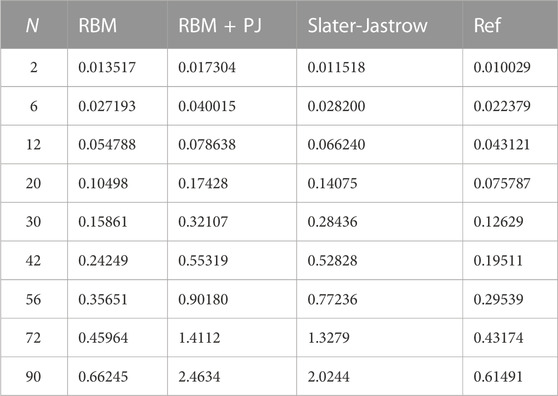
TABLE 1. CPU time per iteration in seconds for various system sizes and ansatzes. The table compliments Figure 3, and computational details are given in the main text.
The ground state energies of two-dimensional quantum dots of various sizes and frequencies are presented in Table 2. The RBM + PJ and Slater-Jastrow ansatzes provide the lowest ground state energies as expected as the correlation factor does explicit satisfy the Kato’s cusp conditions. The relative errors with respect to diffusion Monte Carlo (DMC) calculations tend to be less than 0.2% for both methods. The various results obtained with the RBM + PJ ansatz show that this ansatz dominates for small quantum dots, but is outperformed by the Slater-Jastrow ansatz for larger systems. We suspect this is due to the fact that the former ansatz is more complex and contains significantly more parameters than the latter, and has therefore a hard time finding the global minimum. The optimization could be improved with a more sophisticated optimization algorithm.
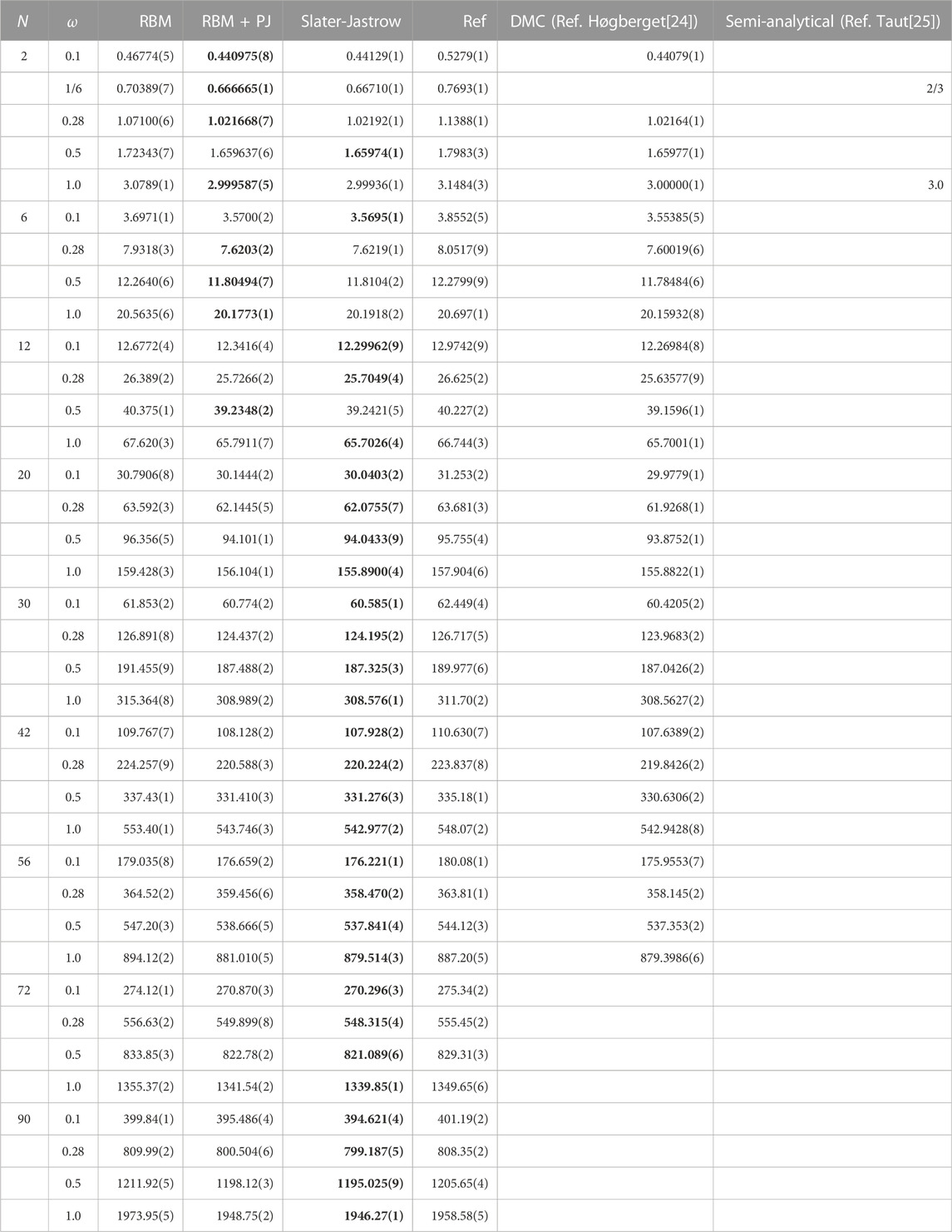
TABLE 2. The ground state energy of two-dimensional quantum dots with N electrons and frequency ω. Other references include diffusion Monte Carlo results taken from Høgberget [24] and semi-analytical results obtained by Taut [25]. The energy is given in Hartree units, and the numbers in parenthesis are the statistical uncertainties in the last digit. Bold values correspond to the lowest ground-state energy obtained in this work. For abbreviations see the text.
For low frequency dots (ω < 0.28), the RBM produces ground state energies lower than the reference energy, but fails for large high frequency dots (N > 6, ω > 0.28). For low frequency dots the interaction energy dominates, and the RBM manages to learn the correlations. For high frequency dots, it is the one-body part of the Hamiltonian which dominates and the interaction part is less important for the final expectation value of the energy. For these systems, the Slater determinant part of the wave function ansatz is the most important one, meaning in turn that the RBM ansatz we have used may not capture well the structure of the single-particle states that define the Slater determinants.
We also note that the reference values are similar to corresponding Hartree-Fock energies up to 30 particles Mariadason [26], which is expected as both approaches try to find the optimal single Slater determinant without a correlation factor.
Some simulations were also performed for the RBM and RBM + PJ ansatzes with sorted network inputs to enforce anti-symmetry under exchange of two particles, as suggested by Ref. Saito [27], among others. Sorted inputs showed promising results, where the ground state energy typically dropped in the fourth or fifth digit. For example, the RBM + PJ ansatz found the ground state energy of a system with N = 30 electrons and ω = 0.5 to be 187.311(1) Hartree. This is lower than the Slater-Jastrow energy. We will investigate this further in a follow-up paper [28].
For the traditional ansatzes that do not contain artificial neural networks, the learning rate determines to a large extent how fast the trial wave function converges towards the true ground state wave function. However, for the RBM and the RBM + PJ approaches, the results are sensitive to the chosen learning rate values. A too large learning rate can easily cause exploding energies, and with a too small learning rate the obtained energies with a given trial function might not converge at all. Our strategy is to find the highest learning rate that does not lead to exploding energies. In general this requires efficient grid searching methods. Here, when the energies have converged, we decrease the learning rate by a factor of 103 and let it run until it converges again. Also, the RBMs tend to converge step-wise, making it hard to know whether or not they have converged.
In Figure 4, the convergence of the local energy is plotted for our four ansatzes for N = 2 electrons. Here the results are compared with analytical calculations for N = 2. A similar behavior is shown for N = 56 electrons and ω = 0.1 in Figure 5. For the N = 2 electrons case, RBM + PJ turns out to be the most accurate ansatz with small absolute errors. During training, the Padé-Jastrow parameter is rather constant, but the adjustment of weights seems important for the model to reach the energy minimum. For larger systems, the Slater-Jastrow ansatz provides a slightly lower energy than the RBM + PJ ansatz. Since the number of inputs for the RBM increases with number of particles, the network contains additional training parameters as we increase the number of electrons. Therefore, the networks get more complex for large quantum dots, and they are naturally harder to train.
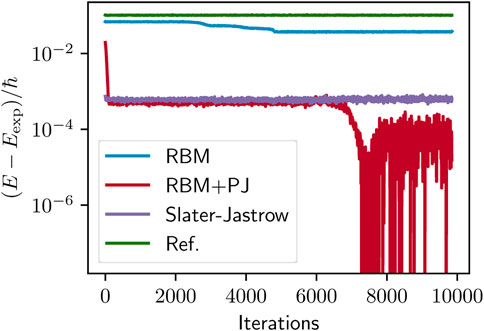
FIGURE 4. Energy convergence for quantum dots with N = 2 and ω = 1/6. The figure shows how the ground state energy approaches the analytical value (Ref. Taut [25]) for various ansatzes.
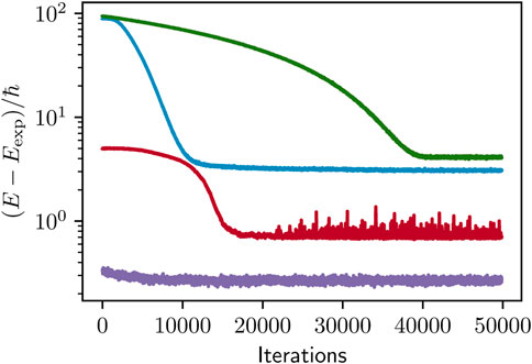
FIGURE 5. Energy convergence for quantum dots with N = 56 and ω = 0.1. The reference value was obtained by Ref. Høgberget [24] using diffusion Monte Carlo. The labeling of the various results is the same as in the previous figure.
The spatial one-body density plots for ω = 1.0 and the RBM and RBM + PJ ansatzes are presented in Figures 6, 7. The electron densities have a wave shape for both ansatzes, with two nodes for N = 2, three nodes for N = 6 and so on similar to those observed in Refs. Ghosal et al. [29]; Høgberget [24]. The RBM seems to exaggerate the states with more distinct peaks (higher peaks and lower wave valleys) compared to the RBM + PJ results. This can be explained by more localized electrons, which becomes even more apparent in low frequency dots (see Figure 8), as the interactions are modelled differently. The RBM would hardly be able to model the correct electron-electron distances, as the network itself is purely linear. The electron density was found to be shape-invariant for high frequency dots (ω > 0.28), with decreasing spatial range as the frequency increases.
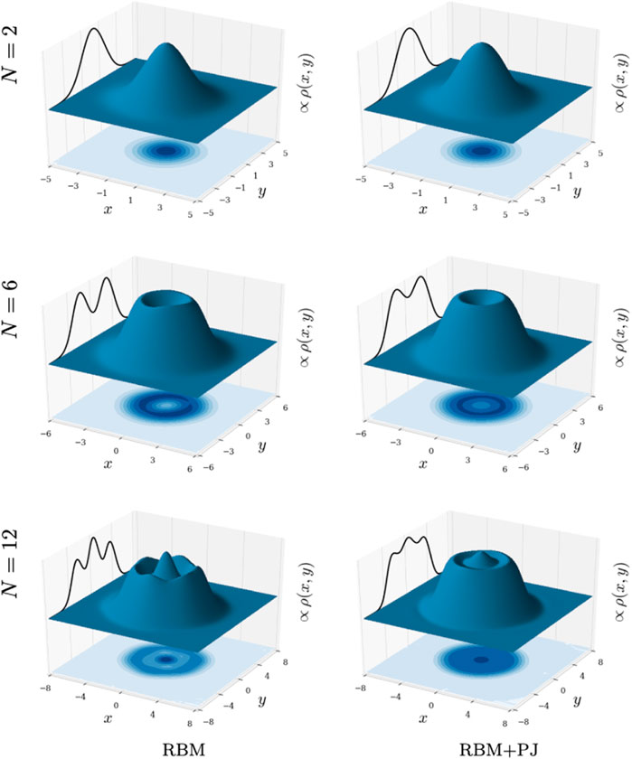
FIGURE 6. Electron density profiles, ρ(x, y), for two-dimensional quantum dots with frequency ω = 0.5 and N = 2, 6 and 12 electrons seen from the top. The surface plot and the contour plot on the xy-plane illustrate the density, and the graph on the yz-plane represents the cross-section through x = 0. They were obtained using RBM (left column) and RBM + PJ (right column), with M = 230 Monte Carlo cycles after convergence. The plots are noise-reduced using a Savitzky-Golay filter. For abbreviations and description of the natural units used, see the main text for more details.
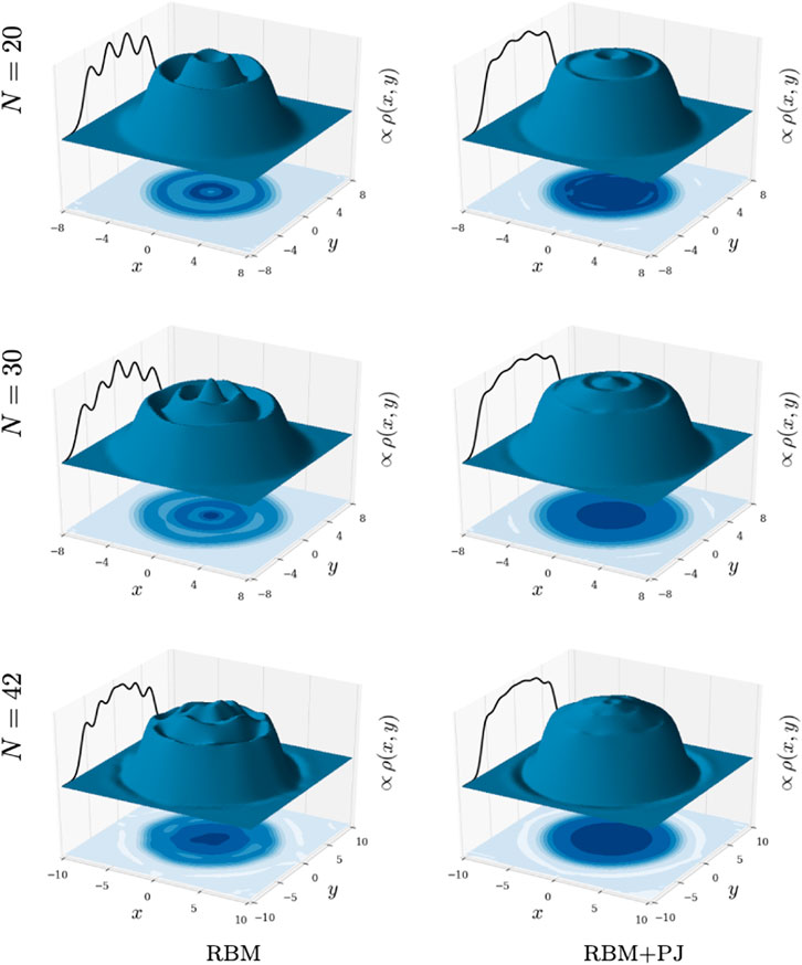
FIGURE 7. Electron density profiles, ρ(x, y), for two-dimensional quantum dots with frequency ω = 0.5 and N = 20, 30 and 42 electrons seen from the top. The surface plot and the contour plot on the xy-plane illustrate the density, and the graph on the yz-plane represents the cross-section through x = 0. They were obtained using RBM (left column) and RBM + PJ (right column), with M = 230 Monte Carlo cycles after convergence. The plots are noise-reduced using a Savitzky-Golay filter. For abbreviations and description of the natural units used, see main text.
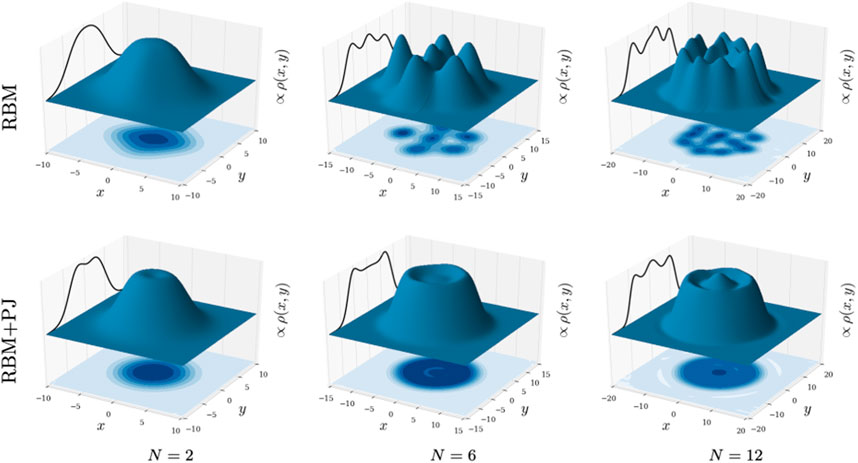
FIGURE 8. One-body density profile, ρ(x, y), of two-dimensional quantum dots with frequency ω = 0.1 and N = 2, 6 and 12 electrons seen from left to right. The ansatzes used are RBM (upper panels) and RBM + PJ (lower panels). The surface plot and the contour plot on the xy-plane illustrate the density, and the graph on the yz-plane represents the cross-section through x = 0. The surface plots are noise-reduced using a Savitzky-Golay filter. For abbreviations and description of the natural units used, see main text.
When reducing the frequency further, the interaction energy dominates over the kinetic energy and harmonic oscillator energy (see Figures 10, 11), and the electrons naturally become more localized. The Padé-Jastrow factor solves this by radially localizing the electrons and conserving the circular symmetry, such that the electrons are confined to specific orbitals. This can be seen from Figure 8, where the spatial one-body density is plotted for low frequency dots (ω = 0.1) and system sizes N = 2, 6 and 12. Radial localization is also what we would expect from the Hamiltonian, which is strictly circular symmetric. On the other hand, the RBM seems to localize the electrons both in radial and angular direction, with the number of electrons corresponding to the number of peaks. This is a nonphysical solution to the problem, and shows that the RBM ansatz breaks down for low frequencies. The RBM + PJ ansatz, on the other hand, confines the electrons in orbitals. Distinct peaks in radial direction is what is expected from Wigner crystallization, which we might see indications of with density parameters rs ≈ 6.7, rs ≈ 1.2, and rs = 0.3 respectively for the three system sizes with the RBM + PJ ansatz. Notice for instance the small “pit” on top of the N = 2 plot for RBM + PJ, which isn’t seen for higher oscillator frequencies. In Figure 9, we have decreased the one-body density even further to ω = 0.01 for N = 2. As expected, the electrons become even more localized and are clearly showing Wigner crystallization effects with a density parameter of rs ≈ 29. For the RBM ansatz, the electrons are strongly localized (in all directions) and the electron densities barely overlap. For the RBM + PJ ansatz, we observe strong orbital confinement where the Wigner crystallization wasn’t the target of this study, but the framework seems capable of a profound study of this phenomenon.
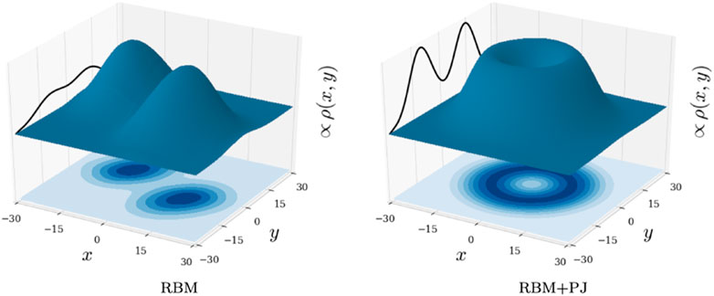
FIGURE 9. One-body density profile, ρ(x, y), of two-dimensional quantum dots with frequency ω = 0.01 and N = 2 electrons. The ansatzes used are RBM (left) and RBM + PJ (right). The surface plot and the contour plot on the xy-plane illustrate the density, and the graph on the yz-plane represents the cross-section through x = 0. The surface plots are noise-reduced using a Savitzky-Golay filter. For abbreviations and description of the natural units used, see main text.
To understand the behavior of the one-body density for various frequencies, we investigate the expectation values of the kinetic energy
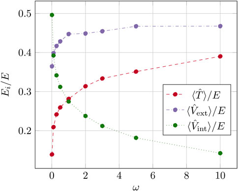
FIGURE 10. Energy distribution for N = 2 electrons for the RBM + PJ ansatz, with frequencies ranging from ω = 0.01 to 10.0.
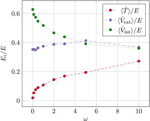
FIGURE 11. Energy distribution for N = 20 electrons for the RBM + PJ ansatz, with frequencies ranging from ω = 0.01 to 10.0.
The quantum dot systems were studied using a general framework for variational Monte Carlo simulations (The code is available on github.com/evenmn/VMaChine). Importance sampling was used to accelerate the simulations Metropolis et al. [31]. To minimize the local energy, we applied the Adam optimizer with β1 = 0.9 and β2 = 0.999 as suggested by Ref. Kingma and Ba [32]. We use an adaptive number of cycles, starting from 220 and then increased to 224 for the ten last iterations after the energy had converged, and further to 230 for the very last iteration to reduce the statistical uncertainty and noise in electron density. The particle step length was chosen to get an acceptance ratio close to 99.5%, spawning from 101 for the smallest and weakest systems to 10–3 for the large and narrow oscillators. The optimal learning rate was found by grid searches, and varied from 101 to 10–5. Both the step length and the learning rate depend strongly on the system and the trial wave function.
For the RBM and RBM + PJ ansatzes, only the raw particle positions were input to the RBM. This choice was made for performance reasons, as inputting processed positions like the electron-electron distances would lead to significantly larger computational efforts, with an increased network complexity.
The Gaussian parameter was initialized to α = 1.0, which is the analytical optimum without interaction. We use Xavier initialization for the RBM weights, putting them all close to zero Glorot and Bengio [33]. The special case with all weights set to zero corresponds to our reference ansatz with α = 1.0. For all the RBMs but the most narrow ones (ω = 1.0), the number of hidden nodes was set to 6, giving 40 to 1272 parameters for the various system sizes. For ω = 1.0, we used H = 12 hidden nodes to achieve a lower energy.
All the simulations were run on Intel Xeon E5-2670 CPUs. In total the computational cost of this project was of the order of 106 CPU hours with largest amount of cycles spent, for obvious reasons, on the largest systems.
We found that the RBM ansatz gives a significantly lower ground state energy than the reference ansatz for low frequency quantum dots. This may indicate that the RBM manages to capture some of the electron-electron correlations. Based on the one-body density plots, the RBM found the electrons to be localized both angularly and radially compared to the ansatzes containing a Padé-Jastrow factor, which confine electrons radially only. For high frequency dots, the RBM fails in the sense that the obtained ground state energy is larger than the reference energy. This can be explained by the fact that when the interactions get less important, the reference ansatz is a good guess. The RBM + PJ ansatz gives energies close to the DMC energies for small quantum dots. The ansatz performance needs to be seen in light of the computational cost, as the ansatzes containing a Padé-Jastrow factor are far more computationally intensive.
From the one-body density and energy distribution plots, it is apparent that the RBM ansatz isn’t able to capture the correlations at the same level as the Padé-Jastrow factor. Because of the linearity of the network, it is impossible for it to compute the distance between the particles, which is crucial to model the interactions correctly. One solution to this could be to input the electron-electron distance into the network, as discussed by Pfau et al. [4], but this would increase the computational intensity. Also, despite including a Slater determinant, the trial wave function is not necessarily anti-symmetric when including an RBM. We performed some simulations where anti-symmetry was forced by sorting the network inputs, which showed promising results in terms of the ground state energy. However, although promising results can be obtained, RBMs are less flexible than general neural networks that make fewer assumptions about the specific mathematical forms of the trial functions. We have encoded explicitly the anti-symmetry via a Slater determinant. Furthermore, two-body correlations are constructed using a Jastrow factor. An RBM with Gaussian distributions is capable of capturing the one-body part of the problem, but is less flexible in finding two-body or more complicated many-body correlations. Although the RBM results reported here are promising compared with existing VMC calculations, recent results with neural networks like those presented in, for example, Refs. Pfau et al. [4]; Cassella et al. [14]; Lovato et al. [9]; Adams et al. [8]; Carrasquilla and Torlai [3] offer much more flexible and promising research venues for deep learning methods applied to many-body problems. Results obtained with deep neural networks for these systems will be presented in a future work [28].
The original contributions presented in the study are included in the article/supplementary materials, further inquiries can be directed to the corresponding author.
The work was conceived by MH-J, JK, and EN. All authors contributed to the article and approved the submitted version.
AL and BF are supported by the U.S. Department of Energy, Office of Science, Office of Nuclear Physics, under contracts DE-AC02-06CH11357, by the NUCLEI SciDAC program, and the DOE Early Career Research Program. MH-J is supported by the U.S. Department of Energy, Office of Science, and office of Nuclear Physics under grant No. DE-SC0021152 and U.S. National Science Foundation Grants No. PHY-1404159 and PHY-2013047. JK is supported by the U.S. National Science Foundation Grants No. PHY-1404159 and PHY-2013047. EN is supported by the Norwegian Research Council under grant 287084.
The authors declare that the research was conducted in the absence of any commercial or financial relationships that could be construed as a potential conflict of interest.
All claims expressed in this article are solely those of the authors and do not necessarily represent those of their affiliated organizations, or those of the publisher, the editors and the reviewers. Any product that may be evaluated in this article, or claim that may be made by its manufacturer, is not guaranteed or endorsed by the publisher.
1Natural units are used with energy given in units of ℏ and length given in units of
2A burn-in period or time refers to the amount of time which is needed before a steady state is reached in a Markov-chain Monte Carlo simulation. When the most likely or steady state has been reached, one can start collecting samples for the stochastic evaluation of the various integrals.
3We have employed a grid of learning rates in terms of powers of ten with negative exponents. Since we have not implemented an adaptive calculation of the learning rates, we search for the optimal results using a grid of decreasing learning rates.
1. Goodfellow I, Bengio Y, Courville A. Deep learning. Cambridge, Massachusetts): The MIT Press (2016).
2. Carleo G, Troyer M. Solving the quantum many-body problem with artificial neural networks. Science (2017) 355:602–6. doi:10.1126/science.aag2302
3. Carrasquilla J, Torlai G. Neural networks in quantum many-body physics: A hands-on tutorial (2021). Available at: https://arxiv.org/abs/2101.11099 (Accessed January 26, 2021).
4. Pfau D, Spencer JS, Matthews AGDG, Foulkes WMC. Ab initio solution of the many-electron Schrödinger equation with deep neural networks. Phys Rev Res (2020) 2:033429. doi:10.1103/PhysRevResearch.2.033429
5. Calcavecchia F, Pederiva F, Kalos MH, Kühne TD. Sign problem of the fermionic shadow wave function. Phys Rev E (2014) 90:053304. doi:10.1103/PhysRevE.90.053304
6. Carleo G, Cirac I, Cranmer K, Daudet L, Schuld M, Tishby N, et al. Machine learning and the physical sciences. Rev Mod Phys (2019) 91:045002. doi:10.1103/RevModPhys.91.045002
7. Boehnlein A, Diefenthaler M, Sato N, Schram M, Ziegler V, Fanelli C, et al. Colloquium: Machine learning in nuclear physics. Rev Moddern Phys (2022) 94:031003. doi:10.1103/RevModPhys.94.031003
8. Adams C, Carleo G, Lovato A, Rocco N. Variational Monte Carlo calculations of A≤4 nuclei with an artificial neural-network correlator ansatz. Phys Rev Lett (2021) 127:022502. doi:10.1103/PhysRevLett.127.022502
9. Lovato A, Adams C, Carleo G, Rocco N (2022). Hidden-nucleons neural-network quantum states for the nuclear many-body problem. Available at: https://arxiv.org/abs/2206.10021 (Accessed June 20, 2022).
10. Hornik K, Stinchcombe M, White H. Multilayer feedforward networks are universal approximators. Neural Networks (1989) 2:359–66. doi:10.1016/0893-6080(89)90020-8
11. Murphy KP. Machine learning: A probabilistic perspective. Cambdridge, Massachusetts): The MIT Press (2012).
12. Hastie T, Tibshirani R, Friedman J. The elements of statistical learning: Data mining, inference and prediction. Berlin): Springer Verlag (2009).
14. Cassella G, Sutterud H, Azadi S, Drummond ND, Pfau D, Spencer JS, et al. Discovering quantum phase transitions with fermionic neural networks. Phys Rev Lett (2023) 130:036401. doi:10.1103/PhysRevLett.130.036401
15. Sieber J, Gehringer J. Quantitative universal approximation bounds for deep belief networks (2022). Available at: https://arxiv.org/abs/2208.09033 (Accessed August 18, 2022).
16. Drummond ND, Towler MD, Needs RJ. Jastrow correlation factor for atoms, molecules, and solids. Phys Rev B (2004) 70:235119. doi:10.1103/physrevb.70.235119
17. Huang C-J, Filippi C, Umrigar CJ. Spin contamination in quantum Monte Carlo wave functions. J Chem Phys (1998) 108:8838–47. doi:10.1063/1.476330
18. Fore B, Kim JM, Carleo G, Hjorth-Jensen M, Lovato A. Dilute neutron star matter from neural-network quantum states. arXiv [Preprint] (2022). doi:10.48550/arXiv.2212.04436
19. Rigo M, Hall B, Hjorth-Jensen M, Lovato A, Pederiva F. Solving the nuclear pairing model with neural network quantum states. Phys Rev E (2023) 107:025310. doi:10.1103/PhysRevE.107.025310
20. Neidinger RD. Introduction to automatic differentiation and MATLAB object-oriented programming. SIAM Rev (2010) 52:545–63. doi:10.1137/080743627
21. Baydin AG, Pearlmutter BA, Andreyevich Radul A, Siskind JM. Automatic differentiation in machine learning: A survey. J Machine Learn Res (2018) 18:1. doi:10.5555/3122009.3242010
22. Hammond BL, Lester WA, Reynolds PJ. Monte Carlo methods in ab initio quantum chemistry. Singapore: World Scientific (1994).
23. Umrigar CJ, Filippi C. Energy and variance optimization of many-body wave functions. Phys Rev Lett (2005) 94:150201. doi:10.1103/physrevlett.94.150201
24. Høgberget J. Quantum Monte Carlo studies of generalized many-body systems. Master’s thesis. Oslo: University of Oslo (2013).
25. Taut M. Two electrons in a homogeneous magnetic field: Particular analytical solutions. J Phys A (1994) 27:1045–55. doi:10.1088/0305-4470/27/3/040
26. Mariadason AA. Quantum many-body simulations of double dot system. Master’s thesis. Oslo: University of Oslo (2018).
27. Saito H. Method to solve quantum few-body problems with artificial neural networks. J Phys Soc Jpn (2018) 87:074002. doi:10.7566/jpsj.87.074002
28. Kim J, Fore B, Nordhagen EM, Lovato A, Hjorth-Jensen M. Deep learning and confined electrons in two dimensions (2022).
29. Ghosal A, Güçlü AD, Umrigar CJ, Ullmo D, Baranger HU. Incipient Wigner localization in circular quantum dots. Phys Rev B (2007) 76:085341. doi:10.1103/physrevb.76.085341
31. Metropolis N, Rosenbluth AW, Rosenbluth MN, Teller AH, Teller E. Equation of state calculations by fast computing machines. J Chem Phys (1953) 21:1087–92. doi:10.1063/1.1699114
32. Kingma DP, Ba J. Adam: A method for stochastic optimization (2014). Available at: https://arxiv.org/abs/1412.6980 (Accessed December 22, 2014).
In this , we will derive the marginal and conditional distributions of a Gaussian-binary restricted Boltzmann machine with the system energy
There are 2N visible units xi with related bias weights ai and H hidden units hj with related bias weights bj. wij are the weights connecting the visible units to the hidden units. The joint probability distribution is given by the Boltzmann distribution
where Z is the partition function,
and β = 1/kBT is the reciprocal temperature that will be fixed to 1. As the marginal and conditional distributions are closely related both for the visible and hidden layer, we present the distributions in sections respective for the two layers.
The distributions of the visible units are used to find properties related to the visible units. If we recall a restricted Boltzmann machine, the transformation between the visible units and the hidden units is
The marginal distribution of the visible units is given by the sum over all possible hidden states, {h} ∈ {0, 1}:
as the hidden units can take binary values only. By inserting the expression of the joint probability distribution from Eq. B1, we obtain
This is what we will use as the marginal distribution of the visible units.
Keywords: quantum dots, many-body physics, Monte Carlo methods, machine learning, Boltzmann machines
Citation: Nordhagen EM, Kim JM, Fore B, Lovato A and Hjorth-Jensen M (2023) Efficient solutions of fermionic systems using artificial neural networks. Front. Phys. 11:1061580. doi: 10.3389/fphy.2023.1061580
Received: 04 October 2022; Accepted: 25 April 2023;
Published: 26 June 2023.
Edited by:
Are Magnus Bruaset, Simula Research Laboratory, NorwayReviewed by:
Tarcísio Marciano Rocha Filho, University of Brasilia, BrazilCopyright © 2023 Nordhagen, Kim, Fore, Lovato and Hjorth-Jensen. This is an open-access article distributed under the terms of the Creative Commons Attribution License (CC BY). The use, distribution or reproduction in other forums is permitted, provided the original author(s) and the copyright owner(s) are credited and that the original publication in this journal is cited, in accordance with accepted academic practice. No use, distribution or reproduction is permitted which does not comply with these terms.
*Correspondence: Morten Hjorth-Jensen, aGplbnNlbkBtc3UuZWR1
Disclaimer: All claims expressed in this article are solely those of the authors and do not necessarily represent those of their affiliated organizations, or those of the publisher, the editors and the reviewers. Any product that may be evaluated in this article or claim that may be made by its manufacturer is not guaranteed or endorsed by the publisher.
Research integrity at Frontiers

Learn more about the work of our research integrity team to safeguard the quality of each article we publish.