 Xinjia Li1
 Wenlian Lu1,2,3,4,5*
- 1School of Mathematical Sciences, Fudan University, Shanghai, China
- 2Shanghai Center for Mathematical Sciences, Fudan University, Shanghai, China
- 3Shanghai Key Laboratory for Contemporary Applied Mathematics, Fudan University, Shanghai, China
- 4Institute of Science and Technology for Brain-Inspired Intelligence, Fudan University, Shanghai, China
- 5Key Laboratory of Computational Neuroscience and Brain-Inspired Intelligence, Fudan University, Ministry of Education, Shanghai, China
The Ensemble Kalman filter (EnKF) is a classic method of data assimilation. For distributed sampling, the conventional EnKF usually requires a centralized server to integrate the predictions of all particles or a fully-connected communication network, causing traffic jams and low bandwidth utilization in high-performance computing. In this paper, we propose a novel distributed scheme of EnKF based on network setting of sampling, called Particle Network EnKF. Without a central server, every sampling particle communicates with its neighbors over a sparsely connected network. Unlike the existing work, this method focuses on the distribution of sampling particles instead of sensors and has been proved effective and robust on numerous tasks. The numerical experiments on the Lorenz-63 and Lorenz-96 systems indicate that, with proper communication rounds, even on a sparse particle network, this method achieves a comparable performance to the standard EnKF. A detailed analysis of effects of the network topology and communication rounds is performed. Another experiment demonstrating a trade-off between the particle homogeneity and performance is also provided. The experiments on the whole-brain neuronal network model show promises for applications in large-scale assimilation problems.
1 Introduction
Data assimilation (DA) is the science of combining system observations with system estimates from a dynamic model to obtain a new and more accurate system description [1]. In DA, the Kalman filter [2] has been regarded as a very effective algorithm to solve state-space representations when the state-space model is linear and Gaussian. As a variant of the Kalman filter, the Ensemble Kalman filter (EnKF) [3] is introduced to deal with the nonlinear state-space model, assuming that all probability distributions are Gaussian. There have been numerous applications involving EnKF, such as physical models of the atmosphere, oceans in geophysical systems [4, 5], and biological science [6].
With complex models and high variability of the dataset, there is a rising demand for deploying DA algorithms in high-performance computing (HPC) in many fields, such as oceanography [7] and neuroinformatics [8–10]. As the system model may be very large, only one computing node is insufficient to compute all particles (samples) to deploy EnKF in HPC. In this situation, the model of each particle can be deployed on more than one node.
When deploying the EnKF in a centralized manner in HPC, a central server is necessary to compute the average of all particles. But there exists two potential challenges: First, computing power or storage space problems may be caused by the scale of the model and exchanged information. Second, traffic jams on the central server may occur during communication [11].
As the main operator for the EnKF is Allreduce, we can deploy it on a fully connected network and use direct all-to-all communication [12] when the number of nodes is not large. As the number of nodes increases, the time to each message hits a floor value determined by the overhead in the switch latencies because a minimum efficient packet size must be used, and it is easy to miss this target size on a large network [13]. This scenario reduces bandwidth utilization and increases the communication cost, motivating industry to deploy the particles on a sparse graph, namely a particle network setting for the EnKF, which is an alternative solution for DA in HPC.
Related work in distributed optimization includes centralized [14, 15] and decentralized algorithms (network setting) [16, 17]. Centralized algorithms assume that a central server is available to integrate the information of all agents and send it back, whereas each agent can only communicate with its neighbors over a local network in decentralized algorithms. Some distributed variants of the Kalman filter, such as the distributed Kalman filter [18–23], distributed particle filter [24], and distributed EnKF [25–27], have recently been introduced as filtering solutions for sensor networks that are robust to link failure and scalable with the network size. However, these methods are designed for sensor networks, and each sensor node runs a local copy of the filter. Thus, to the best of our knowledge, there is no method focusing on particle networks for EnKF rather than sensors networks to handle the problem of DA in HPC.
In this paper, we propose a decentralized EnKF, named Particle Network EnKF for data assimilation in systems with linear and nonlinear measurements. The most relevant work to this current study is the decentralized filter distributing a centralized Kalman filter based on average consensus filters [22]. However, unlike the previous research on the distributed filters, this paper focuses on the distribution of particles instead of sensors from a new perspective, which has many significant applications in large-scale computing.
The Particle Network EnKF deploys particles in a decentralized way and performs reasonable calculations on each node. The particles are distributed in a network and maintain local estimates of global variables, such as the average of predicted states and observations, which can be obtained by communicating with their neighbors over several communication rounds. Then, the algorithm calculates the particles’ Kalman gains and update predicted states. In this way, there is no need for a central server, and it has a lower communication cost than the EnKF with a fully connected network.
To illustrate the proposed method, we experiment on various systems with the Particle Network EnKF, including the Lorenz-63 system with known or unknown parameters and the Lorenz-96 system with nonlinear measurement. The Particle Network EnKF can achieve comparable performance to the EnKF with fewer communication costs, even on a sparse graph. Moreover, we analyze the effects of critical hyperparameters on the Particle Network EnKF and propose an indicator called the gossiping rate to indicate the effects of network topology and communication rounds on the precision and homogeneity.
To determine the trade-off between the paticle homogeneity and precision of filtered states, we modify the Particle Network EnKF, where the particle heterogeneity can be upper bounded theoretically. Finally, we demonstrate the superior performance of the Particle Network EnKF on a large-scale computing application, the whole-brain neuronal network model, where the EnKF fails, as the state update for each particle is computationally intensive.
Contributions. Our contributions are summarized as follows:
• We propose a novel decentralized EnKF called the Particle Network EnKF. From a new perspective, we focus on the distribution of particles instead of sensors as done in the existing works, achieving comparable performance to the EnKF with fewer communication costs, even on a sparse network.
• We define an indicator called the gossiping rate, α, to quantify the combined effects of the network topology and multiple communication rounds. Moreover, we explore the trade-off between the particle homogeneity and precision of the filtered states.
• We test the Particle Network EnKF on the whole-brain neuronal network model, where our method shows promises for applications in large-scale assimilation applications.
The paper is organized as follows. Section 2 reviews the standard EnKF and presents the proposed Particle Network EnKF. Section 3 illustrates the effectiveness of the proposed method on the Lorenz-63 and Lorenz-96 systems and discusses the effects of the network topology and multiple communication rounds. Also, we explore the trade-off between the particle homogeneity and precision in Section 4. In Section 5, we test the Particle Network EnKF on a practical large-scale application (i.e., the whole-brain neuronal network model). Finally, we summarize the work in Section 6.
2 Ensemble Kalman filter and particle network EnKF
In this section, we review the preliminary knowledge of EnKF and introduce the proposed Particle Network EnKF in detail. The proposed method is designed for distributed sampling in lager-scale DA problems, which is obviously different from previous work for sensor networks.
2.1 Ensemble Kalman filter
The EnKF, a variant of the Kalman filter, is a typical method to handle nonlinear systems in DA. The standard EnKF’s context assumes a system [28] with m-dimensional state vector x and n-dimensional observation vector y:
where f and g are system function and measurement function respectively, and wk and vk are Gaussian noises with covariance matrix Q and R. If the measurement function g is linear, the measurement formula can be simplified to
where
The EnKF employs an ensemble approach to address the nonlinear system. Specifically, it uses the Monte Carlo method to choose numerous state points in the initialization step and conducts a prediction step and update step iteratively.
Initialization Step. The filter starts by randomly drawing the initial ensembles by independently sampling N particles
Then, for time steps k = 1, …, K, the filter obtains estimates of the state at the current time step k using the state estimates from the last time step k − 1 in the prediction step and then refines the state estimates with the current prediction and observation in the update step.
Prediction Step. In the prediction step, the EnKF builds the predicted states by drawing N independent samples from the signal model and calculates the mean of the predicted states:
where wi,k−1 is drawn from the distribution of the systemic noise
Update Step. In this step, the EnKF first calculates the observations using the measurement function and obtains the Kalman gain matrix Kk. Then, the predicted states is updated according to the Kalman gain matrix. For each particle i, the update step can be formulated as follows [29]:
where vi,k is drawn from
The update step for nonlinear measurement was proposed by [29], which is completed by rewriting the Kalman gain in the standard EnKF update step Eq. 4. The motivation of Eq. 3 is that the measurement function g in standard EnKF must be linear, which might cause concerns when the nonlinear measurement function is challenging to be linearized [30]. The update step for nonlinear measurement Eq. 3 has been widely used to manage systems with nonlinear measurement functions.
The two update steps are equivalent when satisfying
Some work [30] has shown that the formula Eq. 5 holds if N is infinite and
2.2 Particle network EnKF
Although the EnKF is an effective method to estimate states in many systems, we cannot use the classic EnKF on certain occasions in real applications. For example, in the DA task for the whole-brain neuronal network model, a single computing node cannot calculate all particles because the computing cost for each particle is too expensive.
We propose the Particle Network EnKF, where each particle can only obtain the information of its neighbors over a locally connected network. We have no access to
We assume that a connected network has local connectivity across particles represented by an undirected graph
where
For a fully connected network, without extra communication, the Particle Netowork EnKF degenerates to the standard EnKF. However, when the network is very sparse, the information of other particles is too little to obtain a credible Kalman gain. Hence, we implement extra communication rounds, where the communication round is denoted by s.
Based on the ideas above, we improve the EnKF algorithm to the Particle Network EnKF both in the prediction and update steps separately.
Prediction Step. In the prediction step, after s rounds of communication, each particle i obtains its estimate
For each particle i ∈ {1, 2, …, N}, the prediction step can be formulated as follows.
Update Step. In the update step, there is no central server to compute the average of
The update step can be formulated as follows:
where
Output. After s rounds of communication, the Particle Network EnKF outputs the final filtered state at step k for each particle.
where
2.3 Gossiping rate
To quantify the combined effects of the network topology and multiple communication rounds, we first review the definition of the gossiping matrix W in Eq. 6, which characterizes information mixing among neighboring particles. We assume that the eigenvalues of W are λ1 > λ2 ≥⋯ ≥ λN, where λ1 = 1 and λN > − 1 (see Lemma 2 in Supplementary Appendix SA in Supplementary Material). As presented in the following, the left eigenvector corresponding to the largest eigenvalue (i.e., 1) of W determines the convergence point of Ws when the number of communication rounds s tends to infinity. Meanwhile, the maximum absolute value of the remaining eigenvalues determines the convergence speed, which is a critical indicator. We define a spectral quantity α for the gossiping matrix W, called the gossiping rate, as follows:
The gossiping rate reflects the sparseness of the network. For example, if the network is fully connected, where all the elements of W are 1/N, the gossiping rate is zero. Moreover, the multiple communication rounds per iteration enhance the gossiping matrix W to Ws and reducing the gossiping rate from α to αs, with s rounds of communication.
Consensus analysis. Let
By Perron Frobenius [31], the left eigenvector
where
Theorem 1. Suppose that W satisfies Eq. 6, and the corresponding graph is connected. Let λ1 > λ2 ≥ λ3 ≥⋯ ≥ λN be the eigenvalues of W, then for any
Theorem 2. Under the condition of Theorem 1, there exists a matrix norm ‖ ⋅‖ such that αs = ‖Ws − W∞‖.
3 Experiment on the Lorenz-63 and Lorenz-96 systems
In this section, we demonstrate the effectiveness of the Particle Network EnKF on the Lorenz-63 system with known and unknown parameters and Lorenz-96 system with nonlinear measurement function.
3.1 Experiment on the Lorenz-63 system with known parameters
In this section, we demonstrate the effectiveness of the Particle Network EnKF on the Lorenz-63 system with known parameters. Some experiments show the effects of the network topology and multiple communication round, which can be presented uniformly by the gossiping rate. The comparison of communication costs with the EnKF illustrates that our method achieves communication-efficiency on sparse networks.
The Lorenz-63 system [34] is formulated as follows:
where σ = 10, ρ = 28, and β = 8/3. Given the initial state
In practice, 1,000 noisy points of the Lorenz-63 system are available. The interval between steps of the Euler method h is 0.01. The states are [x,y,z]T with a system noise covariance Q = 0.3 ×I3×3, and the initial states in this experiment are [1.0,3.0,5.0]T. The parameters are [σ,ρ,β]T without any noise. The observation noise covariance R is 4, and the states are filtered at every time step.
For both the EnKF and the Particle Network EnKF, the number of particles N is 50. We randomly sample the initial points of a multivariate Gaussian distribution with mean [1.5,2,6]T and covariance matrix p = 2 × I3 × 3. Then, we repeat each experiment 100 times to obtain credible results. As a baseline, the EnKF reduces the root mean square error (RMSE) of signal from 2.01 to 0.865 ± 0.012 with the nonlinear update step (3) and 0.863 ± 0.012 with the linear update step (4).
We generate a connected random communication graph using an Erdős-Rényi (ER) graph [35, 36] with the probability of connectivity of p = 0.2. For the proposed method, the communication round s is 3. The mean RMSE for all particles is 0.872 ± 0.014, and the top-1 RMSE is 0.865 ± 0.014 using the nonlinear update step while 0.874 ± 0.015 and 0.868 ± 0.015 by the linear update step. Therefore, even randomly choosing a particle for a sparse graph, the Particle Network EnKF can reduce the signal error to a comparable level to the EnKF.
If the measurement function is linear, the two update steps with linear and nonlinear measurement have similar performance, while the latter is more generalized. In the following experiments, we only present the results of the Particle Network EnKF with the nonlinear update step (3).
3.1.1 Effects of the network topology
The network topology is a vital factor determining the performance of the Particle Network EnKF. Hence, we experiment to demonstrate how different network topologies affect the performance with only one communication round, including ER graphs with different probabilities of connectivity p and Watts-Strogatz (WS) graphs [37] using the rewriting probability of 0.3 and a different mean degree k.
Regardless of the type of network topology, the mean RMSE steadily degrades with increasing connections (Figures 1A,B). However, a denser network leads to higher communication costs. The proposed method can achieve comparable performance to the EnKF even on a sparse network.
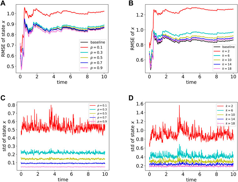
FIGURE 1. Mean RMSE and standard deviation of
As mentioned above, the Particle Network EnKF has no access to the global average of all particle outputs, and every particle i holds its filtered state
3.1.2 Effects of multiple communication round
For each particle of the sparse network, the information from its neighbors is often scarce, limiting reasonable estimates of the global average. For example, a significant gap exists between the WS graphs with k = 2 and k = 6 (Figure 1B) due to the lack of information exchanged in the sparse graph. To improve the performance of the Particle Network EnKF with sparse graphs, we use multiple communication rounds in the prediction and update steps within every time step. We generate four graphs and experiments to demonstrate the effects of multiple communications including ER graphs, WS graphs, random regular (RR) graphs [38] with different degree d, and Barabási-Albert (BA) graphs [39] with different values of m.
To be deployed in HPC and reduce computing and storage costs, our Particle Network EnKF acquires the neighbors’ information instead of the detailed global information, which is the reason why EnKF is better than our Particle Network EnKF at the beginning of communicating on sparse networks as Figure 2A shows. However, with the communication round s between particles increases, the acquired information is more complete, which helps the Particle Network ENKF approach ENKF to achieve better particle homogeneity and reduce the mean RMSE.
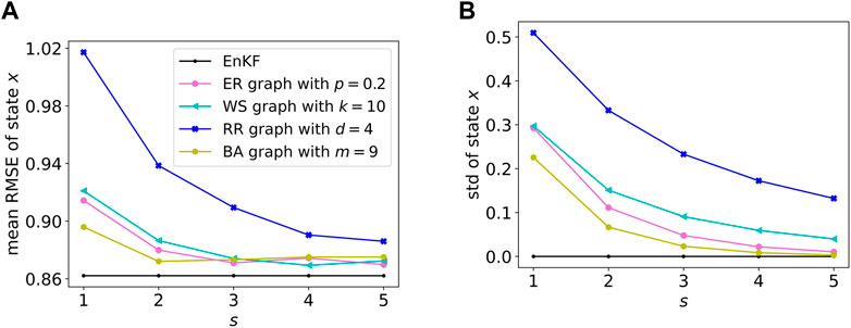
FIGURE 2. Mean and standard deviation of all particles with different communication rounds s. (A) Shows the Mean RMSE of particles and (B) is the plot the mean of {stdk, k = 1, 2, …, K} to display the homogeneity performance.
We apply the standard deviation stdk of
3.1.3 Combined effects of network topology and multiple communications
In this section, we illustrate that the combined effect of the network topology and multiple communication rounds both intrinsically reduce αs, which is discussed in Theorem 1 and Theorem 2. In detail, a denser network indicates a smaller α value, whereas more communication rounds indicate a larger value of s.
We randomly generate four graph types (i.e., ER graphs with p = 0.1, 0.2, …, 1.0; WS graphs with p = 0.3, k = 2, 4, …, 20; RR graphs with r = 2, 4, …, 20; and BA graphs with m1 = 1, 2, …, 10).
The effects on the RMSE. When the communication round s is 1, only a single communication occurs. As α rises, the network becomes sparser, the RMSE becomes larger (Figure 3A). When s communication rounds occur between particles, the gossiping matrix W of the graph becomes Ws and the gossiping rate α reduces to αs (Figure 3B). Moreover, as 0 ≤ α < 1, more communication rounds lead to a smaller gossiping rate. The RMSE decreases with multiple communication rounds as the gossiping rate decreases.
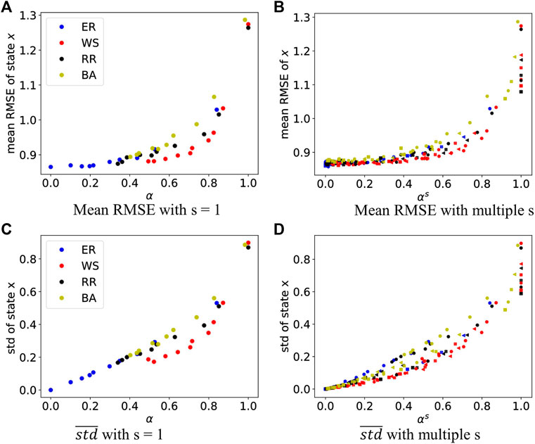
FIGURE 3. Mean RMSE and mean standard deviation of state x on the Lorenz-63 system. Colors represent different network types, and shapes represent communication rounds s. The markers for s = 1, 2, 3, 4, 5 are a circle, left triangle, filled X, hexagon, and square respectively. (A,B) display the mean RMSE of state x along with the gossiping rate. (C,D) are plots of the mean std to illustrate the influence of the gossiping rate on the homogeneity.
In general, the Particle Network EnKF can improve performance by designing a denser network or executing more communication rounds. Both two methods reduce the gossiping rate αs. To obtain a better trade-off between performance and communication, given a connected network, we can obtain the gossiping rate α and then empirically choose a proper s to get a good performance with fewer communication costs.
The Effects on homogeneity. If the communication round is set to be one, a smaller gossiping rate α indicates better homogeneity (Figure 3C). Nevertheless, a slight gap exits between different topologies. For example, the WS graphs achieve better homogeneity than the ER and BA graphs with the same gossiping rate. When the gossiping rate α becomes αs with multiple communication rounds, the particles have a better homogeneity as the gossiping rate declines. The gap between different network topologies under the same gossiping rate shrinks as the network becomes denser (Figure 3D).
3.1.4 The communication cost compared to EnKF
In this section, we compare the communication cost of the Particle Network EnKF and EnKF to show our method can achieve communication-efficiency on sparse networks.
When deployed the EnKF algorithm on any connected network with N nodes, whose topology is known, it needs N(N − 1) communications. As for particle Network EnKF, every node only collects the information from its neighbors. Thus, the communication cost of a node is proportional to its degree and the communication round s. Table 1 shows the communication cost on the network with N = 50 nodes in some experiments on Lorenz-63.
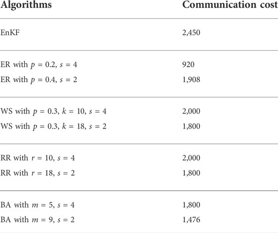
TABLE 1. The communication cost of EnKF and our method with different communication round s for some networks.
Figure 4 shows the logarithm of the ratio of the communication cost between EnKF and our method with different αs on a network with α. For most networks that are not too dense (i.e., αs > 0.1), the Particle Network EnKF is significantly communication-efficient than EnKF, as it does not require the particles to send their information to all the other nodes.
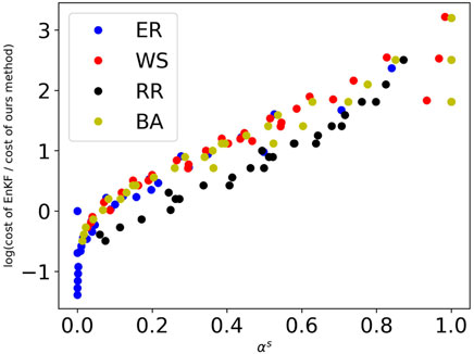
FIGURE 4. The logarithm of the ratio of communication cost between EnKF and our proposed method with different αs. As the sparsity of the network increases (i.e., αs > 0.1), the communication cost of EnKF is much more than the Particle Network EnKF.
3.2 Experiment on the Lorenz-63 system with unknown parameters
In this section, we explore the ability to assimilate the parameters [σ,ρ,β]T of the Particle Network EnKF. The dataset is the same as that in Section 3.1, and only x is observable. The difference is that we assume the parameters [σ,ρ,β]T are unknown, and the variables to be estimated are [x,y,z,σ,ρ,β]T instead of [x,y,z]T.
The system noise covariance Q and measurement covariance R are diag{0.3, 0.3, 0.3, 0, 0, 0} and 4, respectively. The number of nodes is also set to be 50. We randomly sample the initial points of a multivariate Gaussian distribution with mean [1.5,2,6,8,30,3]T and covariance matrix p = 3 × I6 × 6. We test 3, 000 steps to filter the noise of states and assimilate the parameters. In this work, for the EnKF, if the standard deviation of the latest 20 consecutive parameters [pT−l+1, pT−l+2, …, pT](p ∈ {σ, ρ, β}) is less than the threshold ϵ = 1e − 3, the parameter p converges. If all parameters converge, then the EnKF converges. The particle network EnKF converges only if all parameters of all particles converge. As the algorithm converges, for every parameter, the estimated error is defined as
In the prediction stage, we fix p as pend and predicted [x,y,z]T for 25 steps. The RMSEs between the predicted xpre, ypre, zpre and true
The EnKF reduces the signal error (RMSE = 2.010) to 0.984 ± 0.014. All experiments converge before 3,000 steps. The mean steps T to converge, called the mean converged steps, is 1,647 ± 129.
For the Particle Network EnKF, we randomly generate a BA graph with m1 = 8. If the communication round is set to be one, 6 out of 100 experiments have not converged before 3, 000 steps. However, if we increase the communication rounds, all 100 experiments converge before 3, 000 steps for these parameters. Specifically, the mean converged steps corresponding to s = 2, 3, 4, 5 are 1,619 ± 360, 1,190 ± 274, 1,080 ± 248, and 1,034 ± 221. The Particle Network EnKF achieves similar performance with the EnKF in the filter and prediction stages (Table 2). Increasing the communication rounds makes the algorithm converge faster but has no significant improvement in filtering the noise.
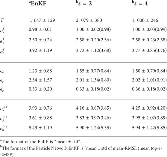
TABLE 2. Detail results of the Lorenz-63 system with unknown parameters.
In the experiments on the Lorenz-63 system with unknown parameters, neither the EnKF nor the Particle Network EnKF can precisely estimate the parameters [σ,ρ,β]T. In this section, we also analyze the possible causes.
For the Particle Network EnKF, as the time step increases, the estimates of the three parameters converge to a relatively stable value (Figure 5). However, the convergence point for each experiment is not always the same but is scattered in a certain range. For example, σ is between 7 and 10.5 where the ground truth is 10. The result of EnKF has a similar property.

FIGURE 5. The estimated parameters [σ,ρ,β]T for the Particle Network EnKF with an ER graph. Only the results of particle 0 are shown.
The EnKF and Particle Network EnKF have a commonality in parameter estimate tasks for the Lorenz-63 system. Thus, we only test the EnKF to determine a reasonable explanation for this phenomenon. If we regard the EnKF as an optimization problem, does it fall into some local optima? To evaluate it, we design an experiment fixing σ and ρ to the ground truths, varying β within certain limitations. Then, we assume that all three parameters are known and implement the EnKF on the Lorenz-63 system with known parameters to get the RMSE of all states [x,y,z]T.
Overall, there is an interval around the ground truth of the β, which allows the algorithm to obtain reasonably good x, y, z with a small RMSE (Figure 6A). However, there are many local optima, into which the EnKF or our Particle Network EnKF may fall (Figure 6B).
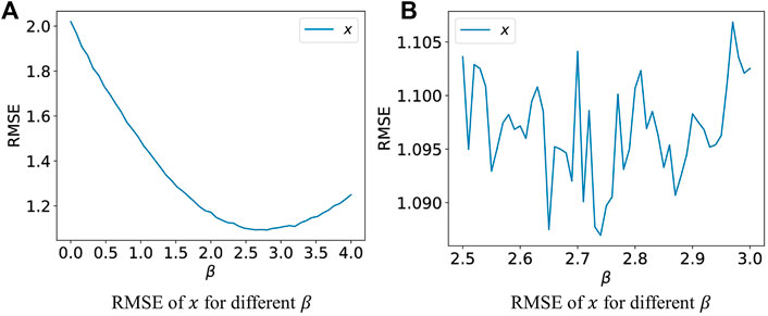
FIGURE 6. Fix σ, ρ and vary β to estimate x, y, z. (A,B) plot the RMSE of the state x with different scaling.
3.3 Experiments on the Lorenz-96 system with nonlinear measurement function
Sections 3.1 and Section 3.2 present the comparable performance of the proposed Particle Network EnKF to ENKF with fewer communication costs on the low-dimensional Lorenz-63 system in filtering noise and estimating parameters. The Particle Network EnKF with update step (8) can also handle systems with nonlinear measurement functions. Hence we apply the Particle Network EnKF on another common system, the Lorenz-96 system [40], which can be formulated as follows:
satisfying F = 8, x−1 = xm−1, x0 = xm, and xm+1 = x1.
The Lorenz-96 system represents a simplified weather system and is a common model in DA. The complexity of the model can be adjusted by m in the system. We consider high dimensional Lorenz-96 system with m = 40 [28, 40], and three variables are observable: x1, x2, and x40. We solve the Lorenz-96 system using a fourth-order Runge-Kutta time integration scheme with a time step of 0.05 [41], which is 6 h in the real world time if the time scale is 5 days [40].
Assume that 1, 000 noisy points of the Lorenz-96 system are available. The states are
We test three measurement functions when generating data and filtering noise: 1) The linear measurement function (linear), g1(x) = [x1, x2, x40]; 2) the rectified linear unit (ReLU) measurement function, g2(x) = max(0, x); and 3) a nonlinear measurement function
We randomly sample the initial points of the multivariate Gaussian distribution with mean
We test the EnKF and the Particle Network EnKF on the ER graph with p = 0.3 and communication rounds s = 3. We repeat each experiment for 50 times.
As a baseline, the EnKF reduces the measurement noise to 1.098 ± 0.014, 1.330 ± 0.018, and 1.376 ± 0.016, respectively for the linear, ReLU, and the nonlinear (i.e. g3(x)) measurement function. For the Particle Network EnKF, the RMSE values are 1.097 ± 0.013,1.330 ± 0.013 and 1.363 ± 0.018. The Particle Network EnKF achieves comparable performance on the assimilation of the high-dimensional system with nonlinear measurements.
4 Trade-off between homogeneity and RMSE
In this section, we explore the trade-off between homogeneity and RMSE by modifying the update step (8). The experiments and theories reveal that the heterogeneity of the updated particles
When the local Kalman gain
where
There is a trade-off between homogeneity and RMSE. By replacing
We offer a mathematical theory regarding the homogeneity for the Particle Network EnKF with Eq. 11 and demonstrate that the difference between particles in each time step can be upper bounded under some conditions where the gossiping rate α and communication rounds s1 are two essential factors.
In this section, the following notation is needed. The symbol ⊗ denotes the Kronecker product, and 0 is a zero matrix. Moreover, λmin(A) is the smallest eigenvalue value of a symmetric matrix A. For a positive define matrix
With s1 communication rounds, Eq. 11 can be described as follows:
where
Let
Then we can rewrite the system Eq. 12 as follows:
Let
We present the following theorem, and the proof is given in Supplementary Appendix SB in Supplementary Material.
Theorem 3. The gossiping rate α of W is defined as Eq. 10. The communication round s1 is defined as in Eq. 11. Define a matrix p = diag{N1, N2, …, NN}, where Ni is the number of neighbors of particle i. If there exists a positive definite matrix
for any
Then, For any k ≥ 1, i, j = 1, 2, …, N, we have
where
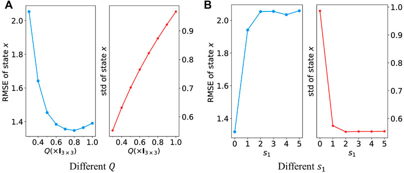
FIGURE 7. RMSE and standard deviation of state x with a different values of Q and s1. (7A) Shows the results with different Q values when filtering and (B) shows the results with different s1 values in Eq. 11. A smaller Q or larger s1 indicates better particle homogeneity.
5 Experiment on the whole-brain neuronal network model
In this section, we experiment on a whole-brain neuronal network model, including 92 brain blocks and 10, 000, 904 neurons. The experiment reveals that the Particle Network EnKF show promises for applications in large-scale computing problems.
5.1 The whole-brain neuronal network model
We assume a whole-brain neuronal network model, composed of basic computing units and a network structure. The basic computing units are neurons and synapses, and the spike signals transmitted between the neurons by synapses are actional potentials (i.e., spikes). Each neuron model receives postsynaptic currents as input and describes the generating scheme of the time points of the action potentials as the output. The network model provides synaptic interactions between neurons by a directed multiplex graph.
We consider the leakage integrate-and-fire (LIF) model to be a neuron. A capacitance-voltage equation describes the membrane potential of neuron i, Vi, when it is less than a given voltage threshold Vth,i, we have
where Ci is the capacitance of the neuron membrane, gL,i denotes the leakage conductance, VL represents leakage voltage, Isyn,i is the synaptic currents and Iext,i is the external stimulus. When Vi = Vth,i at
Afterward, Vi is again governed by Eq. 11.
We consider an exponentially temporal convolution to be this map
where gu,i is the conductance of the synapse type u of neuron i, Vu represents the voltage of the synapse type u,
We simulate the brain of a human based on prior knowledge, and divide the brain into 92 blocks [42], where LGN is from [43]. We propose a network model of hierarchical random graphs with constraints and multiple edges, to represent the neuron pairwise synaptic connections. To generate the neuronal connectivity, we divide the 10,000,904 neurons into 92 brain blocks where the number is proportional to the gray volume obtained by the sMRI. The ratio of the number of excitation neurons to that of the inhibitory neurons is 4:1. The in-degree of each neuron is 100, where 50% are from the excitation neurons out of this block, 30% are from excitation neurons within this block, and the others are from the inhibitory neurons within this block. For each neuron, the probability of connecting to other blocks is determined by the diffusion tensor imaging (DTI) data.
Once the mean fire rate of each block is obtained, the measured blood oxygenation level dependent (BOLD) responses can be calculated [44] for each brain block.
5.2 The experiments on signal filtering
In this experiment, only one BOLD signal is measurable for each brain block. The measurement variance is 1e − 6. In this experiment, we use an ER graph with p = 0.3 and repeat each experiment 10 times to obtain stable results.
Each brain block model must be run on 1.5 NVIDIA GeForce GTX 1080 Ti GPUs. We also use sparsity to optimize the communication between nodes, according to the generated random graph. For N = 30 particles, 45 GPUs are used in the experiments.
The Particle Network EnKF reduces the noise of measurements (RMSE = 1.436e − 3) to 4.745e − 4 ± 7.559e − 5 with a communication round and 4.294e − 4 ± 6.931e − 5 with multiple communication rounds where s = 3. The Particle Network EnKF reduces the measurement noise to a low level for all 92 brain blocks (Figure 8).
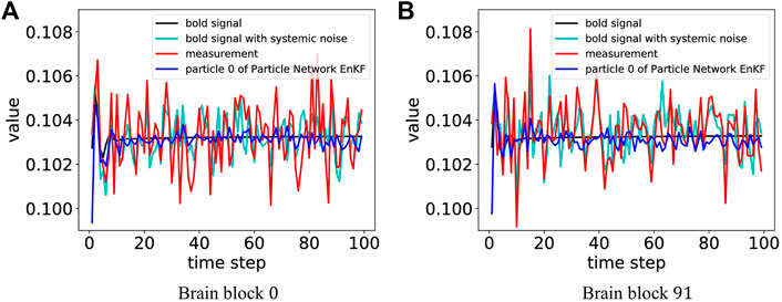
FIGURE 8. The results of the filtering bold signal for blocks 0 and 91. For the Particle Network EnKF, we only depict the performance of particle 0 as an example. (A) shows the result for the brain block 0 and (B) shows the result for the brain block 91.
The ground truth of the parameter to assimilate gAMPA,i is 1.027e − 2. Table 3 lists the detailed mean and top-1 RMSE of the parameters for the particles. The proposed method estimates the parameters with a small relative error. The results reveal that the Particle Network EnKF shows promises for applications application in large-scale computing problems.
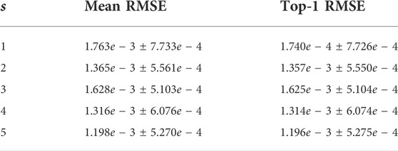
TABLE 3. Mean and top-1 RMSE of the parameter gAMPA,i.
6 Conclusion
We propose a particle-based distributed EnKF, called Particle Network EnKF in this paper. It assumes that the particle of the EnKF has no access to global information and can only communicate with its neighbors over a network. In this way, there is no central node to store and calculate states from all particles, and the network can be very sparse. Hence, the proposed method can address the limitation of storage space or low bandwidth utilization in large-scale computing. Moreover, it can achieve comparable performance to the EnKF with fewer communication costs in filtering the states and assimilating the parameters. In theory, denser networks and more communication rounds improve the performance by changing the gossiping matrix, which is indicated by the gossiping rate. The proposed method is very practical and effective in large-scale calculations and avoids the bandwidth and storage space limitations.
Data availability statement
The raw data supporting the conclusion of this article will be made available by the authors, without undue reservation.
Author contributions
All authors listed have made a substantial, direct, and intellectual contribution to the work and approved it for publication.
Funding
This work was supported by the National Key R&D Program of China (No. 2018AAA0100303), National Natural Sciences Foundation of China under Grant (No. 62072111), and Shanghai Municipal Science and Technology Major Project under Grant 2018SHZDZX01 and ZJLab.
Conflict of interest
The authors declare that the research was conducted in the absence of any commercial or financial relationships that could be construed as a potential conflict of interest.
Publisher’s note
All claims expressed in this article are solely those of the authors and do not necessarily represent those of their affiliated organizations, or those of the publisher, the editors and the reviewers. Any product that may be evaluated in this article, or claim that may be made by its manufacturer, is not guaranteed or endorsed by the publisher.
Supplementary material
The Supplementary Material for this article can be found online at: https://www.frontiersin.org/articles/10.3389/fphy.2022.998503/full#supplementary-material
References
1. Vetra-Carvalho S, van Leeuwen PJ, Nerger L, Barth A, Altaf MU, Brasseur P, et al. State-of-the-art stochastic data assimilation methods for high-dimensional non-Gaussian problems. Tellus A: Dynamic Meteorology and Oceanography (2018) 70:1–43. doi:10.1080/16000870.2018.1445364
2. Kalman RE. A new approach to linear filtering and prediction problems. J Basic Eng (1960) 82:35–45. doi:10.1115/1.3662552
3. Evensen G. Sequential data assimilation with a nonlinear quasi-geostrophic model using Monte Carlo methods to forecast error statistics. J Geophys Res (1994) 99:10143–62. doi:10.1029/94JC00572
4. van Leeuwen PJ. Particle filtering in geophysical systems. Mon Weather Rev (2009) 137:4089–114. doi:10.1175/2009MWR2835.1
5. Rabier F. Overview of global data assimilation developments in numerical weather-prediction centres. Q J R Meteorol Soc (2005) 131:3215–33. doi:10.1256/qj.05.129
6. Jang J, Jang K, Kwon HD, Lee J. Feedback control of an hbv model based on ensemble kalman filter and differential evolution. Math Biosci Eng (2018) 15:667–91. doi:10.3934/mbe.2018030
7. Teruzzi A, Di Cerbo P, Cossarini G, Pascolo E, Salon S. Parallel implementation of a data assimilation scheme for operational oceanography: The case of the medbfm model system. Comput Geosciences (2019) 124:103–14. doi:10.1016/j.cageo.2019.01.003
8. Izhikevich EM, Edelman GM. Large-scale model of mammalian thalamocortical systems. Proc Natl Acad Sci U S A (2008) 105:3593–8. doi:10.1073/pnas.0712231105
9. van Albada SJ, Rowley AG, Senk J, Hopkins M, Schmidt M, Stokes AB, et al. Performance comparison of the digital neuromorphic hardware spinnaker and the neural network simulation software nest for a full-scale cortical microcircuit model. Front Neurosci (2018) 12:291. doi:10.3389/fnins.2018.00291
10. Painkras E, Plana LA, Garside J, Temple S, Galluppi F, Patterson C, et al. Spinnaker: A 1-w 18-core system-on-chip for massively-parallel neural network simulation. IEEE J Solid-state Circuits (2013) 48:1943–53. doi:10.1109/JSSC.2013.2259038
11. Lian X, Zhang C, Zhang H, Hsieh CJ, Zhang W, Liu J. Can decentralized algorithms outperform centralized algorithms? A case study for decentralized parallel stochastic gradient descent. In: NIPS’17: Proceedings of the 31st International Conference on Neural Information Processing Systems. Red Hook, NY, USA: Curran Associates Inc. (2017). p. 5336–46.
12.[Dataset] Duato J. Interconnection networks : An engineering approach/josé duato, sudhakar yalamanchili, lionel ni (1997).
13. Zhao H, Canny J. Kylix: A sparse allreduce for commodity clusters. In: 2014 43rd International Conference on Parallel Processing (2014). p. 273–82. doi:10.1109/ICPP.2014.36
14. Shamir O, Srebro N, Zhang T. Communication efficient distributed optimization using an approximate Newton-type method. In: 31st International Conference on Machine Learning (2013).
15. Boyd S, Parikh N, Chu E, Peleato B, Eckstein J. Distributed optimization and statistical learning via the alternating direction method of multipliers. FNT Machine Learn (2011) 3:1–122. doi:10.1561/2200000016
16. Li B, Cen S, Chen Y, Chi Y. Communication-efficient distributed optimization in networks with gradient tracking and variance reduction. arXiv preprint arXiv:1909.05844 (2019).
17. Koloskova A, Stich SU, Jaggi M. Decentralized stochastic optimization and gossip algorithms with compressed communication. CoRR abs/1902.00340 (2019).
18. Mahmoud M, Khalid HM. Distributed kalman filtering: A bibliographic review. IET Control Theor & Appl (2013) 7:483–501. doi:10.1049/iet-cta.2012.0732
19. Zhou Y, Li J. Distributed sigma-point kalman filtering for sensor networks: Dynamic consensus approach. In: 2009 IEEE International Conference on Systems, Man and Cybernetics (2009). p. 5178–83. doi:10.1109/ICSMC.2009.5346001
20. Msechu EJ, Roumeliotis SI, Ribeiro A, Giannakis GB. Decentralized quantized kalman filtering with scalable communication cost. IEEE Trans Signal Process (2008) 56:3727–41. doi:10.1109/tsp.2008.925931
21. Olfati-Saber R. Distributed kalman filter with embedded consensus filters. In: Proceedings of the 44th IEEE Conference on Decision and Control (2005). p. 8179–84. doi:10.1109/CDC.2005.1583486
22. Talebi SP, Werner S. Distributed kalman filtering and control through embedded average consensus information fusion. IEEE Trans Automat Contr (2019) 64:4396–403. doi:10.1109/TAC.2019.2897887
23. Kar S, Moura JMF. Gossip and distributed kalman filtering: Weak consensus under weak detectability. IEEE Trans Signal Process (2011) 59:1766–84. doi:10.1109/TSP.2010.2100385
24. Yu JY, Coates MJ, Rabbat MG. Graph-based compression for distributed particle filters. IEEE Trans Signal Inf Process Netw (2019) 5:404–17. doi:10.1109/tsipn.2018.2890231
25. Kazerooni M, Shabaninia F, Vaziri M, Vadhva S. Distributed ensemble kalman filter for multisensor application. In: 2013 IEEE 14th International Conference on Information Reuse Integration (IRI) (2013). p. 732–5. doi:10.1109/IRI.2013.6642544
26. Sirichai P, Yamakita M. Using ensemble kalman filter for distributed sensor fusion. Trans ISCIE (2013) 26:466–76. doi:10.5687/iscie.26.466
27. Shahid A, Üstebay D, Coates M. Distributed ensemble kalman filtering. In: 2014 IEEE 8th Sensor Array and Multichannel Signal Processing Workshop (SAM) (2014). doi:10.1109/SAM.2014.6882379
28. Hamilton F, Berry T, Sauer T. Ensemble kalman filtering without a model. Phys Rev X (2016) 6:011021. doi:10.1103/PhysRevX.6.011021
29. Houtekamer PL, Mitchell HL. A sequential ensemble kalman filter for atmospheric data assimilation. Monthly Weather Rev (2001) 129:123–37. doi:10.1175/1520-0493(2001)129<0123:ASEKFF>2.0.CO;2
30. Tang Y, Ambandan J, Chen D. Nonlinear measurement function in the ensemble kalman filter. Adv Atmos Sci (2014) 31:551–8. doi:10.1007/s00376-013-3117-9
31. Godsil C, Royle GF. Algebraic graph theory. No. Book 207 in graduate texts in mathematics. Berlin, Germany: Springer (2001).
32. Xiao L, Boyd S. Fast linear iterations for distributed averaging. Syst Control Lett (2004) 53:65–78. doi:10.1016/j.sysconle.2004.02.022
33. Aysal TC, Yildiz ME, Sarwate AD, Scaglione A. Broadcast gossip algorithms for consensus. IEEE Trans Signal Process (2009) 57:2748–61. doi:10.1109/TSP.2009.2016247
34. Lorenz EN. Deterministic nonperiodic flow. J Atmos Sci (1963) 20:130–41. doi:10.1175/1520-0469(1963)020-0130:DNF-2.0.CO;2
37. Watts DJ, Strogatz SH. Collective dynamics of ’small-world’ networks. Nature (1998) 393:440–2. doi:10.1038/30918
38. Steger A, Wormald NC. Generating random regular graphs quickly. Comb Probab Comput (1999) 8:377–96. doi:10.1017/s0963548399003867
39. Barabási AL, Albert R. Emergence of scaling in random networks. Science (1999) 286:509–12. doi:10.1126/science.286.5439.509
40. Lorenz E. Predictability: A problem partly solved. In: Seminar on predictability, 4-8 september 1995. ECMWF, Vol. 1. Shinfield Park, Reading: ECMWF (1995). p. 1–18.
41. Ott E, Hunt B, Szunyogh I, Zimin A, Kostelich E, Corazza M, et al. A local ensemble kalman filter for atmospheric data assimilation. Tellus A (2004) 56:415–28. doi:10.1111/j.1600-0870.2004.00076.x
42. Tzourio-Mazoyer N, Landeau B, Papathanassiou D, Crivello F, Etard O, Delcroix N, et al. Automated anatomical labeling of activations in spm using a macroscopic anatomical parcellation of the mni mri single-subject brain. NeuroImage (2002) 15:273–89. doi:10.1006/nimg.2001.0978
43. Rolls ET, Huang CC, Lin CP, Feng J, Joliot M. Automated anatomical labelling atlas 3. NeuroImage (2020) 206:116189. doi:10.1016/j.neuroimage.2019.116189
Keywords: EnKF, data assimilation, gossip algorithms, decentralized sampling, large-scale problem
Citation: Li X and Lu W (2022) Particle network EnKF for large-scale data assimilation. Front. Phys. 10:998503. doi: 10.3389/fphy.2022.998503
Received: 20 July 2022; Accepted: 18 August 2022;
Published: 28 September 2022.
Edited by:
Duxin Chen, Southeast University, ChinaCopyright © 2022 Li and Lu. This is an open-access article distributed under the terms of the Creative Commons Attribution License (CC BY). The use, distribution or reproduction in other forums is permitted, provided the original author(s) and the copyright owner(s) are credited and that the original publication in this journal is cited, in accordance with accepted academic practice. No use, distribution or reproduction is permitted which does not comply with these terms.
*Correspondence: Wenlian Lu, d2VubGlhbkBmdWRhbi5lZHUuY24=