Reproducible phantom for quality assurance in abdominal MRI focussing kidney imaging

Quality assurance (QA) in magnetic resonance imaging (MRI) requires test objects. ‘Phantoms’ provided by MR manufacturers are homogeneously filled spheres or cylinders, and commercially available products are often too small for abdominal imaging, particularly for enlarged polycystic kidneys. Here we present the design, manufacturing and testing of a dedicated, yet versatile, abdominal MRI phantom, that can be reproduced with relatively low costs. The phantom mimics a human abdomen in size and shape and comprises seven test fluids, representing various tissue types at 3 T. The conductivity and permittivity of the test fluids match the average abdomen and kidney with a relative permittivity (ε) 65 and 72 as well as conductivity 0.6 and 0.7 S/m, respectively. The T₁ and T₂ relaxation times cover healthy average abdomen and kidney tissue values (T_1(abd): 856 ms and T_1(kid): 1,106 ms; T_2(abd): 52 ms and T_2(kid): 67 ms), intermediate (T₁: 1,183 ms and 1,271 ms; T₂: 128 and 189 ms), and disease values for (polycystic) kidney (T₁: 1,428 ms, 1,561 ms and 1763 ms; T₂: 319 ms, 424 and 647 ms). T₁ and T₂ relaxation times were stable over 73 weeks. Our reasonably priced, durable and reproducible abdominal phantom enables single and multi-center QA for future collaborative studies aiming for various challenges around abdominal and, particularly, kidney imaging.

Introduction

Abdominal magnetic resonance imaging (MRI) in clinical routine is challenging, mainly due to the large volume, strong susceptibility changes which lead to e.g., signal dephasing, B₁ heterogeneity, and organ motion causing artefacts. Some of these challenges are traditionally dealt with by using lower field strengths (≤1.5 T), while MRI systems with 3 T are mostly used in high-end clinical examinations in neurology and skeletal radiology as those provide higher sensitivity, which is turned into higher spatial resolution and specificity [1, 2]. However, state-of-the-art abdominal MRI research has to meet the challenges of applying higher field strengths (3 T) to deliver quantitative functional and structural information for the translation into clinical practice. For renal MRI, this has been proposed in detail by a European Cooperation of Science and Technology (COST) Action PARENCHIMA (CA 16103, renalMRI.org) [3], with several reviews on the most promising MRI techniques [4–7]. Furthermore, technical recommendations were recently shared with the community, including sequence acquisition schemes and parameters, orientations, and quality control (e.g., adjusting for B₀ and B₁ inhomogeneities) [8–12]. All those protocols are designed to be short and to maintain patients’ comfort (breath-hold duration), because they need to be included into established/diagnostic qualitative abdominal MRI protocols. Therefore, these fast-imaging protocols need to be validated against gold standard protocols, which take up to several hours. This shows the need for further optimizations and standardizations of various renal MRI protocols, in particular for MR relaxometry, as no final consensus was reached on some important key points for clinical renal T₁ and T₂ mapping. For example, two different T₁ mapping schemes were proposed (modified Look-Locker inversion recovery (MOLLI) and classic inversion recovery (IR) with echo planar imaging (EPI) readout), and for T₂ mapping no final consensus was reached regarding the optimal acquisition scheme (multi-echo (ME) spin-echo (SE), gradient and spin-echo (GRASE), or T₂ preparation) [11].

Image quality can be optimized either via in vivo testing or in phantom measurements, and both solutions have strengths and limitations. In vivo measurements allow for testing stability against physiological motion (breathing, cardiac motion), field inhomogeneities and susceptibility artefacts. However, these effects are different between subjects, and therefore, in vivo measurements cannot be linked to a ground truth of e.g., relaxation times. In contrast, phantoms allow for comparing the results of, e.g., fast MRI sequences to be optimized to ground truth data established with carefully calibrated measures. Clearly, B₀ and B₁ fields as well as susceptibility effects remain constant in phantoms and ensure reproducibility throughout measurements. This renders phantom measurements ideal for investigating sequence parameters. But a significant limitation is that most commonly available phantoms, such as MR system manufacturer’s phantoms, are not designed to meet the challenge for quality assurance (QA) of clinical abdominal imaging [13]. Firstly, they generally do not provide the relevant range of required relaxation times, and secondly, they also do not mimic the abdomen with its required large field of view (FOV). And commercial phantoms are often relatively small and spherically designed for brain imaging, which reduces B₀ and B₁ inhomogeneities. Therefore, they are often unsuitable to reproduce the B₀ and B₁ inhomogeneity effects associated with the larger FOV in abdominal MRI. These, in particular the RF wave effects that induce spatial heterogeneity of the flip angle, typically cause hyperintense and hypointense regions in abdominal MRI [see (Figure 1)], and have the potential to affect accuracy of T₁ and T₂ mapping methods [14].

FIGURE 1

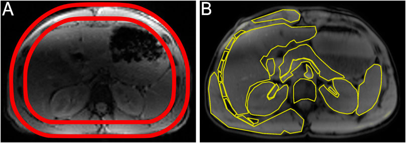
FIGURE 1. Design and shape of the abdominal phantom. (A) Axial T₁ weighted image of the upper abdomen of a healthy volunteer used to define the shape of the abdominal phantom (red drawing on top of the axial image). (B) Axial T₁ weighted image of a healthy volunteer with segmented areas of the upper abdomen (liver, spleen, pancreas, vessels, duodenum, and various bones and muscles). These areas were used to calculate the averaged dielectric properties and relaxation times of the intra-abdominal test fluid. The images show two slices from different positions in the same volunteer and exemplify non-uniformities caused by inhomogeneous excitation B₁ due to wave effects (hypointense: central dark region), and receive coil sensitivities (hyperintense: bright region near surface), as often seen in uncorrected abdominal MRI.

Here we present our novel, anatomically shaped abdominal phantom, designed with relatively low budget requirements. It features good reproducibility and versatility for different abdominal applications. This phantom is designed to mimic enlarged Autosomal-Dominant Polycystic Kidney Disease (ADPKD) kidneys [15, 16] using test fluids with calibrated T₁ and T₂ relaxation times as well as appropriate permittivity and conductivity properties. The phantom enables reproducible tests of renal MRI sequences, especially for relaxometry, to meet the described application challenges around evaluating chronic kidney diseases and healthy controls.

Materials and methods

Abdominal phantom

An axial image of the upper abdomen of a healthy volunteer (male, body mass index 24.2, age 26 years) was used as a reference to mimic the shape and dimensions of our abdominal phantom (Figure 1). Two transparent plastic cylinders, made from thermoplastic polymethyl methacrylate (PMMA, acrylic glass), with a diameter of 300 and 250 mm, respectively, and a wall thickness of 5 mm each, were used to create a two-compartment phantom. The outside compartment represents the subcutaneous fat and the inner compartment the intra-abdominal cavity. These cylinders were placed in a heating chamber for deformation. To approximate the upper abdomen’s shape, a pre-cut sandwich of cardboards and polystyrene together with a wooden board on the posterior surface was used (Figure 2A). A weight was placed on the anterior surface, and some parts were locally rewarmed to fit. The formed cylinders were then glued together on a flat PMMA plate to close the phantom on one side (includes: tempering, removal from grease: ACRIFIX® TC 0030, adhesion: ACRIFIX® 2R 0190 and 3% ACRIFIX® CA 0020; EVONIK, Röhm GmbH, Weiterstadt, Germany). Four screw threaded holes were placed in this end-plate and closed with PMMA screws for filling or cleaning the outer compartment [see (Figure 3C)]. On the opposite side only the outer compartment was closed with a pre-cut plate glued in place, whereas a removable lid was constructed to access the inner compartment. Two threaded holes were placed on the lid, providing access without the need to fully open the lid [e.g., for filling the inner compartment; see (Figure 3A)].

FIGURE 2

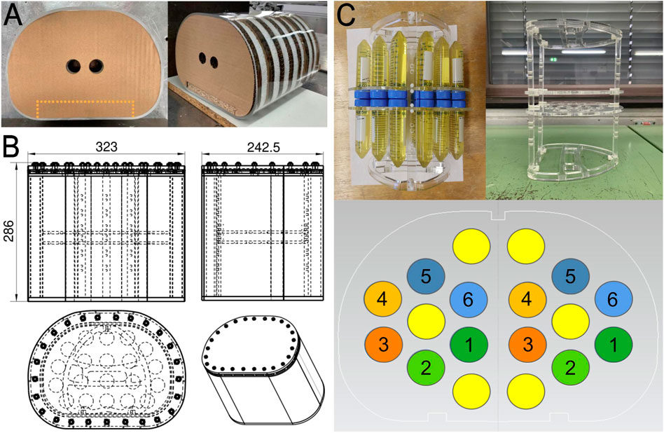
FIGURE 2. Abdominal phantom design and building. (A) Procedures of shaping the acrylic glass cylinders after being in the heating cabinet with a sandwich of pre-cut cardboards, polystyrene, and pressed wood (dashed cutout). (B) Technical drawings of the abdominal phantom (dimensions in mm). Further technical drawings are depicted in the Supplementary Materials. (C) Inside the abdominal phantom is an inlay with a set of test tubes, equally arranged on both sides and mirrored top to bottom. One set is composed of six kidney test fluids, hexagonally arranged in circular order from lowest T₁ and T₂ in kidney sample one to the highest relaxation times in kidney sample six [see (Table 1)]. Corn oil filled samples are shown in yellow. The purpose of this arrangement is to test varying SNR across the image, due to B₁ fields and receive coil proximity using different pulse sequences.

FIGURE 3

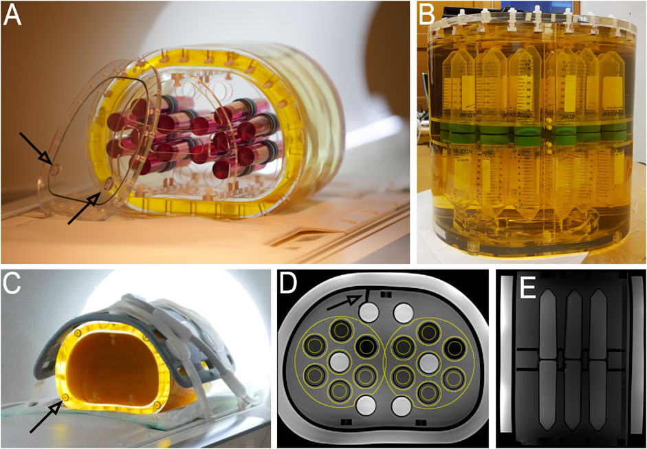
FIGURE 3. Abdominal phantom structure and composition. (A) Final construction and illustration of the abdominal phantom. For visualisation purposes coloured test tubes are placed on the inlay holder. The outer compartment is filled with corn oil, simulating subcutaneous fat. The arrows point at the screw threaded holes to access the inner compartment without the need to lift the whole lid. (B) Photo of the final abdominal phantom immediately after filling. The kidney test samples are submerged into the intra-abdominal test fluid (transparent before gelling). (C) Phantom measurement setup with the 18-element flexible body coil array on top, and the 32-element spine coil array on the bottom. The arrow points at one of the four screw threaded holes, which was placed to access the outer compartment. (D) Axial T₁ weighted image of the phantom with 14 ROIs (yellow circles). The air bubble (arrow) is caused by shrinkage upon cooling of the intra-abdominal test fluid (arrow). (E) Sagittal T₂ weighted image of the phantom.

For the inner compartment a holder (inlay) was designed (Figure 2C). This inlay holds two laser-cut PMMA discs, which allows for inserting 50 ml conical centrifuge tubes with a diameter of 30 mm and length of 115 mm (50 ml FALCON® tube, Corning Incorporated, New Jersey, United States). Screw threads were placed on the holder bars to set the axial distance between the discs allowing them to lock two test tubes on top of each other. All phantom materials were tested for material compatibility with the used test fluids (in compliance with the norm DIN 53435:1983).

Temperature phantom

Repeated MR acquisitions were applied over several hours to increase the temperature inside the phantom, which is known to increase T₁ and decrease T₂ [17, 18]. To assess the impact of temperature on T₁ and T₂ an additional, but down-scaled, 3.5 L abdominally shaped phantom was created without a complex inner structure. Two small tubes (5 cm length, 2 mm outer diameter, and 1 mm inner diameter) were put inside to guide optical temperature sensors (OmniLink; Qualitrol Instruments, Neoptix, NY, United States) into the core of this phantom.

Test fluids

The outer compartment of the phantom was filled with 4 L corn oil. In the inner compartment, 24 test tubes containing each 60 ml of different test fluids were arranged hexagonally in four groups on each side of the holder (left/right/head/feet); non-yellow circles in (Figure 2C). Each of the four hexagonally arranged sets comprises six test tubes with the same set of T₁ and T₂ values. In addition, three test tubes containing corn oil [marked yellow in (Figure 2C)] were placed on each side (in total 720 ml of corn oil), potentially useful for evaluating, e.g., fat saturation or chemical shift artifacts. The holder with all 36 test tubes was submerged in 8.5 L test fluid representative for intra-abdominal tissue, which also matches T₁ and T₂ values of healthy kidney (Figure 3B).

Permittivity and conductivity of various abdominal tissues were taken from previous publications [19, 20]. The mean intra-abdominal T₁ and T₂ relaxation time was based on [21], and relevant renal T₁ and T₂ relaxation times were taken from [7]. To extrapolate the mean dielectric properties and mean T₁ and T₂ relaxation time of the intra-abdominal test fluid an axial image of the upper abdomen at the level of the renal arteries of a healthy subject was used to segment the area of all relevant tissues [averaging the values from various organs; see (Figure 1B)]. The resulting dielectric properties of the intra-abdominal and kidney test fluids as well as T₁ and T₂ relaxation times are summarized in (Table 1).

TABLE 1

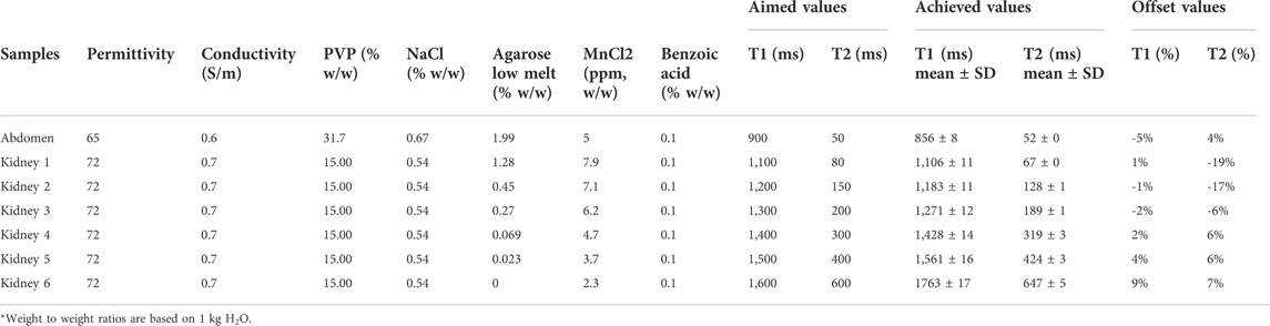
TABLE 1. Summary of composition of all abdominal and kidney test fluids: targeted permittivity, conductivity, concentration of polyvinylpyrrolidone (PVP), sodium chloride (NaCl), agarose, manganese (II)-chloride (MnCl₂) tetrahydrate and benzoic acid. Targeted and achieved (measured) T₁ and T₂ values. Achieved mean and SD values for T₁ and T₂ relaxation times are based on 28 measurements over 73 weeks. The Abdomen and Kidney 1 test fluids represent normal T₁ and T₂ values. Kidney 2 and 3 feature intermediate renal T₁ and T₂ values. Kidney 4 to 6 exhibit renal T₁ and T₂ values typical for disease.

Tissue-equivalent dielectric properties were created with solutions of 15.00% w/w and 31.7% w/w polyvinylpyrrolidone (PVP K 30 extra pure, M = 40,000 g/mol; Carl Roth, Karlsruhe, Germany), and 0.54% w/w and 0.67% w/w sodium chloride for the kidney and intra-abdominal test fluids, respectively. Weighing was done repeatedly on calibrated Sartorius LP620P (d = 1 mg; Sartorius, Goettingen, Germany) and Sartorius BP121S (d = 0.1 mg; Sartorius, Goettingen, Germany). Weight to weight ratios of all test fluids are based on 1 kg H₂O, summarized in (Table 1). The sodium chloride concentration was achieved by mixing sterile water for injection (1,000 ml Aqua Ecotainer®; B. Braun, Maria Enzersdorf, Austria) and 0.9% sodium chloride solution for injection (1,000 ml NaCl 0.9% Ecotainer®; B. Braun, Maria Enzersdorf, Austria). In addition, 0.1% w/w benzoic acid (M = 122.1 g/mol; Carl Roth, Karlsruhe, Germany) was used for conservation. They were created in several volumes of 1 L on different days in a closed container using a vibrating table at room temperature for up to 24 h. After successful dissolution, each test fluid was degassed using a rotary vane pump and stored in air and water tight plastic containers (reused/cleaned 1,000 ml Aqua and NaCl 0.9% Ecotainer®). In total, 9 L of the intra-abdominal test fluids and 2 L of kidney test fluids were created.

After 3 months these test fluids were further doped with agarose (ROTI®agarose Low Melt; Carl Roth, Karlsruhe, Germany) and manganese (II)-chloride (MnCl₂) tetrahydrate (M = 197.91 g/mol; Merck & Co., Kenilworth, New Jersey, United States) to achieve the desired T₁ and T₂ relaxation times. For this, these fluids were filled in empty and cleaned disinfectant flasks (mikrozid AF liquid 750 ml; Schülke and Mayr, Vienna, Austria), because they were sufficiently air and water tight during the heating phase (up to 95°C). They were submerged in a heated water bath and rotated manually for 6 hours until the agarose was fully dissolved. Upon increased pressure the flasks were shortly ventilated.

The MnCl₂ concentrations required to obtain the desired T₁ relaxation times were approached by assuming a linear dependence of the T₁ relaxation rate (R₁) on [MnCl₂] [22]. The desired T₂ relaxation times were then adjusted by adding agarose in iterative steps. These initial samples were stored in syringes (10 ml) to seal them properly for storage in the scanner room and during relaxivity measurements. Once all required concentrations were defined, the final samples were created. These solutions were immediately degassed and stored in air and water tight plastic containers (1,000 ml Ecotainer® for intra-abdominal test fluid, and in 50 ml FALCON® tubes for kidney test fluids). Kidney test fluids were first created to measure the stability of solutions regarding T₁ and T₂ relaxation times over a period of 9 weeks (11 MR measurements: three on Wednesdays, seven on Saturdays, one on Sunday), prior to placing them in the final phantom.

For the filling of the final phantom, the kidney test fluids and oil-filled test tubes were placed on the inlay holder and put into the phantom. The intra-abdominal test gels were carefully remelted (95°C warm water bath, only shortly ventilated to account for increased pressure due to evaporation). After that, the melted intra-abdominal test fluid was poured into the inner compartment of the phantom, and the lid was closed. During the cooling period of about 4 hours, the intra-abdominal test fluid was topped up using the threaded holes [see (Figure 3A)]. Illustrations of the abdominal phantom are shown in (Figure 3). All kidney test fluids were filled into the test tubes without any entrapped air.

Six weeks after the filling of the phantom, relaxometry measurements were continued to assess the long-term stability of the intra-abdominal and kidney test fluids for 73 weeks [28 MR measurements: three on Thursdays, 18 on Fridays and seven on Saturdays, see (Figure 5)].

FIGURE 5

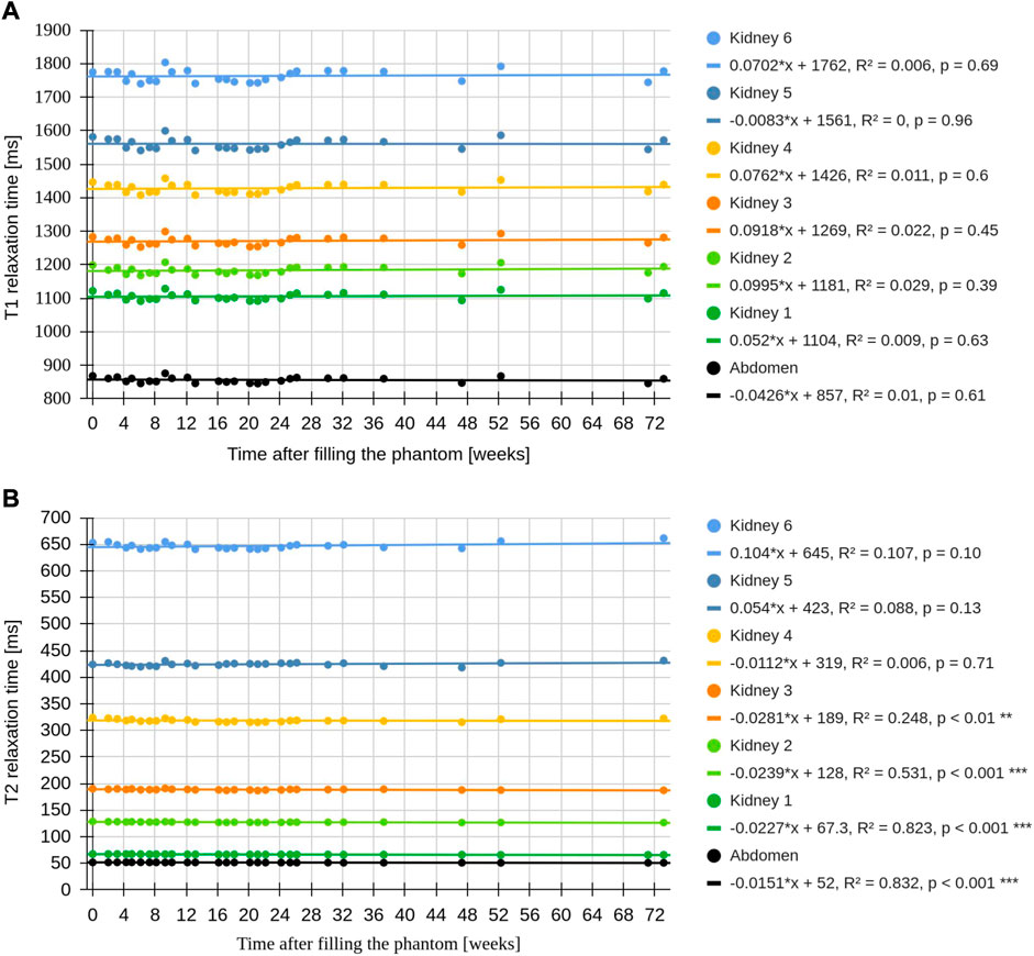
FIGURE 5. Time course of T₁ and T₂ relaxation times of the abdominal phantom. (A) Linear regression of T₁ relaxation times showed no significant drift over the time course of 73 weeks. SD of T₁ values are within 1% of the mean, corresponding to a maximum temperature change of 1°C (based on the temperature phantom measurements). (B) Linear regression of T₂ relaxation times showed a very small but significant decline in the intra-abdominal, kidney test fuild one, two and three. Kidney test fluid five and six showed no relevant drift. The mean and SD of T₁ and T₂ of the test fluids are summarized in (Table 1).

MR setup and sequences

Measurements were performed on a whole-body 3 T scanner (PrismaFit; Siemens Medical Solutions, Erlangen, Germany) equipped with a 32-element spine coil array (Spine 32; Siemens Medical Solutions, Erlangen, Germany) and an 18-element flexible body coil array (Body 18; Siemens Medical Solutions, Erlangen, Germany). The manufacturer’s automated abdominal and standard B₀ shimming mode and volume-selective and patient-specific B₁ shimming mode were used for T₁ and T₂ measurements, respectively. T₁ relaxation time measurements were performed using a 2D single-slice inversion recovery (IR) turbo spin echo (TSE) sequence with TR = 10,000 ms, TE = 8.4 ms, voxel size: 0.75 × 0.75 × 5 mm³, turbo factor: 7, echo train per slice: 47, readout bandwidth 352 Hz/px, slice selective inversion pulse, inversion times (TI): 50, 100, 200, 400, 600, 1,000, 1,300, 1,600, 1900, 2,500, 3,500, 5,000, 9,000 ms. Total acquisition time (TA) for T₁: 104 min. T₂ relaxation times were measured using a 2D single-slice multi-echo (ME) sequence derived from the Carr-Purcell-Meiboom-Gill (CPMG) sequence with TR = 10,000 ms, TE = 8 ms, voxel size 0.75 × 0.75 × 5 mm³, readout bandwidth: 352 Hz/px, echo train length: 32, four separate T₂ mappings with different echo spacings to cover the given range of T₂ values: 8 ms (for intra-abdominal and kidney test sample one), 10 ms (for kidney test sample two), 27 ms (for kidney test sample three to five), and 50 ms (for kidney test sample six) [23, 24]. Total TA for all four T₂ measurements: 216 min.

The abdominal phantom was placed inside the scanner to simulate a patient lying supine, and all measurements, i.e., images, were performed axially to test the long term stability. The phantom was centered on the MRI table using the scanner’s laser visor and the initial iso-center was placed between the test tube sets, ensuring day-to-day reproducible positioning. The alignment was verified with localizers, and a fixed protocol was used for automatic alignment of shimming volumes and imaging slices. For axial imaging, the iso-center was moved to the FOV. Separate sagittal measurements were performed to quantify the uniformity of the test solutions (iso-centre was placed between the test tube sets).

The phantom was stored at constant room temperature (23°C) in the MRI room, measured with a Type-K sensor (FLUKE 289 True RMS Multimeter; Fluke Corporation, Washington, United States), as this is the common operating temperature for many MRI scanners worldwide. During MR measurements the ventilation inside the scanner bore (generally in operation, also during in vivo measurements) was set to maximum to remove heat from the coils and phantom.

Signal-to-noise (SNR) measurements were performed to validate the methods for T₁ and T₂ relaxation time calculations. For T₁, temporal SNR measurements using the same IR-TSE sequence as for T₁ relaxation time measurements, but with a fixed TI = 50 ms, were used. Consecutively, an additional T₁ relaxation time measurement was performed to normalize the temporal SNR measurement to M_z = 1 (based on r_a; see also MR data processing). For T₂, the SNR of the T₂ weighted magnitude images were calculated.

MR data processing

The signal model for T₁ relaxation time measurements using a IR SE scheme with instantaneous RF pulses and no off-resonances is defined as

$M_z=M_0\frac{1-\cos \left({\theta }_1\right)\cos \left({\theta }_3\right){\mathrm{e}}^{-\frac{TR}{T_1}}-\cos \left({\theta }_1\right)\left[1-\cos \left({\theta }_3\right)\right]{\mathrm{e}}^{-\frac{TR-\frac{TE}{2}}{T_1}}-\left[1-\cos \left({\theta }_1\right)\right]{\mathrm{e}}^{-\frac{TI}{T_1}}}{1-\cos \left({\theta }_1\right)\cos \left({\theta }_2\right)\cos \left({\theta }_3\right){\mathrm{e}}^{-\frac{TR}{T_1}}}(1)$

with the following RF and readout sequence: ${\theta }_{\mathrm{1}}-TI-{\theta }_{\mathrm{2}}-\frac{TE}{\mathrm{2}}-{\theta }_{\mathrm{3}}-\frac{TE}{\mathrm{2}}-T_D$, and a fixed $TR=TI+TE+T_D$ [25, 26]. M_z is the magnetization in z direction, M₀ reflects the proton density (and a machine-dependent proportionality constant), θ₁ is the initial 180° RF pulse, θ₂ is a 90° RF pulse and θ₃ is a consecutive 180° RF pulse. This leads to different signal intensities (S (TI_n)), as M_Z is sampled at different TI_n [26]:

$S\left({TI}_n\right)=K{M}_z={\mathrm{e}}^{\mathrm{i}\mathrm{\Phi }}\left(r_a+r_b{\mathrm{e}}^{-\frac{{TI}_n}{T_{\mathrm{1}}}}\right)(2)$

with Φ ranging from -π to π as the phase of K, with contributions from T₂ and coil sensitivities, where

$r_a=\left|K\right|M_0\frac{1-\cos \left({\theta }_1\right)\cos \left({\theta }_3\right){\mathrm{e}}^{-\frac{TR}{T_1}}-\cos \left({\theta }_1\right)\left[1-\cos \left({\theta }_3\right)\right]{\mathrm{e}}^{-\frac{TR-\frac{TE}{2}}{T_1}}}{1-\cos \left({\theta }_1\right)\cos \left({\theta }_2\right)\cos \left({\theta }_3\right){\mathrm{e}}^{-\frac{TR}{T_1}}}(3)$

and

$r_b=-\left|K\right|M_0\frac{1-\cos \left({\theta }_1\right)}{1-\cos \left({\theta }_1\right)\cos \left({\theta }_2\right)\cos \left({\theta }_3\right){\mathrm{e}}^{-\frac{TR}{T_1}}}(4)$

The (Eq. 2) has four real-valued unknowns: Φ, r_a, r_b, and T₁. Using only magnitude IR-SE images for T₁ relaxation time measurement with TR >> T₁ (Eq. 2), becomes

$\left|S\left(TI\right)\right|=\left|r_a+r_b{\mathrm{e}}^{\frac{-TI}{T_{\mathrm{1}}}}\right|(5)$

with r_a, r_b and T₁ being real-valued.

Barral’s model [26] uses a reduced-dimension non-linear least squares with polarity restoration (RD-NLS-PR) algorithm, modelling the signal dependence on TI [S(TI)], to solve T₁ in (Eq. 5). In short, it takes advantage of knowing that TI increases monotonically and S(TI_n) approaches an initial point of zero, and thereafter S(TI) increases. This defines until when the polarity of S(TI) must be reversed. This simplification and the use of a grid search allows a fast 1D search for T₁.

The T₂ magnitude signals at each TE [S(TE)] were fitted mono-exponentially as

$S\left(TE\right)=S_0{\mathrm{e}}^{\frac{-TE}{T_2}}(6)$

S₀ reflects the proton density (and a machine-dependent proportionality constant) and the first echo was omitted [27].

The acquired DICOM files were post-processed using MATLAB (R2020b; The MathWorks, Natick, MA, United States) together with MRIcron [28] and qMRLab [29]. All calculated maps were loaded into ImageJ [30], where 14 ROIs were defined within each kidney test sample, and in the surrounding intra-abdominal test fluid (Figure 3D), and mean values were extracted. Statistical calculations were processed with R [31]. Linear regressions were applied to assess the T₁ and T₂ long term stability of the test samples in the abdominal phantom, and for temperature related R₁ and T₂ relaxation rate (R₂) changes in the temperature phantom. Paired t-tests were used to compare mean T₁ and T₂ in the abdominal phantom before and after repeated relaxometry.

Results

A human size abdominal shaped phantom with two compartments and an inlay holder for 36 test tubes was successfully manufactured (Figures 2, 3). The material and machine costs are summarized in (Table 2) and sum up to about 1,300 €.

TABLE 2

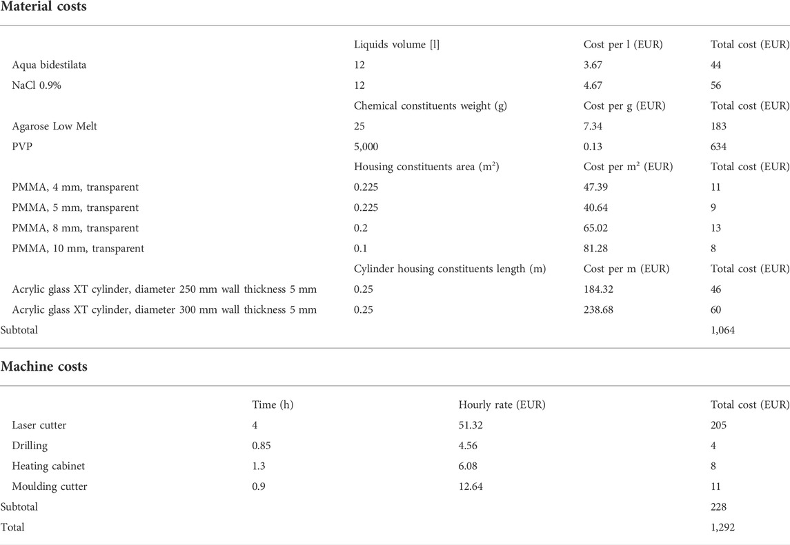
TABLE 2. Material and machine cost calculation of the abdominal phantom.

The tissue-equivalent dielectric intra-abdominal and kidney test fluids, prior to doping with agarose and MnCl₂, were created within 1 month by the liter. Relaxation time measurements of the undoped intra-abdominal test fluid resulted in T₁ = 1,327 ± 18 ms and T₂ = 1,267 ± 25 ms, and undoped kidney test fluids had T₁ = 1970 ± 8 ms and T₂ = 1827 ± 16 ms.

Results of the initial long-term stability test of the final kidney samples prior to insertion into the abdominal phantom are summarized in (Figure 4) with linear regressions of the T₁ relaxation times showing no significant trend. T₂ relaxation times of the kidney samples one, two, three and five showed a significant but small decrease, and the other samples showed no significant trend over time.

FIGURE 4

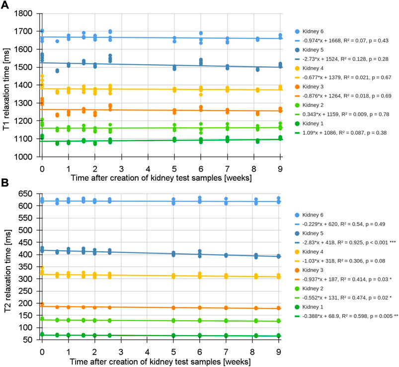
FIGURE 4. Stability of kidney test fluids prior to the insertion into the abdominal phantom. Each kidney test fluid was filled in four separate tubes [one for each set; see (Figure 2)]. (A) Linear regression of T₁ relaxation times of the kidney test samples showed no significant trend with respect to time. (B) Linear regression of T₂ relaxation times of the kidney samples one, two, three and five show a small but significant decline. The other samples exhibited no significant trend. Over the course of 9 weeks the mean T₁ and T₂ values were -0.7% and -4.8% below the targeted values [see also (Table 1)].

Despite having carefully avoided entrapping air during filling, the large volume of the intra-abdominal test fluid shrunk during the cooling period, creating a small air bubble in the enclosed phantom, which is visible at the anterior surface as a crack (Figure 3D).

Results of the long-term stability measurement of relaxometry for the intra-abdominal and kidney test fluids over 73 weeks are shown in (Figure 5). Linear regressions of these results exhibited no significant relationship with respect to time for all T₁ relaxation times, and for T₂ relaxation times of kidney samples four, five and six. A non-substantial but significant decline of T₂ values was present for the intra-abdominal test fluid and kidney samples one, two and three. The standard deviation (SD) of the mean T₁ values is <1% of the mean. Sagittally measured relaxation times were uniform in head-foot direction, with a mean offset of 1.0% compared to axially measured relaxivities.

Using the temperature phantom we directly measured a T₁ increase of 2.2% and a T₂ decrease of 0.7% per °C temperature increase [temperature range for T₁: 22.9–25.4°C; R² = 0.999; p < 0.001; temperature range for T₂: 23.3–25.5°C; R² = 0.997; p < 0.001; see (Supplementary Figure S2)]. Extrapolating these results to the abdominal phantom with repeated T₁ and T₂ relaxation time measurements over 7 h resulted in a mean 3.0% increase of T₁ and a paired t-test exhibited significance in all test samples (mean differences ranging from 24.9 to 57.1 ms, p < 0.001). A T₂ decrease of 0.7% was found in samples with shorter T₂ (intra-abdominal and kidney test fluid one; mean differences ranging from -0.5 to -0.2 ms with p < 0.001), while samples with longer T₂ showed a 1.8% increase (kidney test sample two to six; mean of the differences ranging from 0.7 to 17.6 ms, p < 0.001). Based on observed T₁ changes, the temperature increase in the abdominal phantom was estimated to be 1.4°C after a 7-h relaxometry measurement session.

Temporal SNR of our T₁ measurements showed noise levels below 0.002 (maximum signal amplitude scaled to 1, cf. Eq. 1) within all 14 ROIs [see (Figure 3D)]. For T₂ measurements, the associated T₂ weighted magnitude images exhibited a mean maximum SNR of 139 ± 31 and mean minimum SNR of 12 ± 10.

None of the test fluids showed signs of bacterial growth or mould formation.

Discussion

We present a novel phantom suitable for quality assurance of abdominal MRI with a large FOV. We fulfilled the requirements of an economically feasible, yet versatile, reproducible, durable and anatomically shaped phantom. The dielectric properties and T₁ and T₂ relaxation times were chosen for quantitative renal MRI, to foster further optimizations and standardizations as laid out by previous publications [3, 7, 8, 11]. In contrast to common designs and commercially available quantitative MRI phantoms [13], such as the National Institute of Standards and Technology (NIST)/International Society of Magnetic Resonance in Medicine (ISMRM) system phantom [32, 33], our abdominal phantom is not spherically shaped like a person’s head but resembles a realistically shaped abdominal torso. Also, the volume and extension of the test samples are significantly bigger, which is important as ADPKD can lead to kidney volumes of up to several liters [16]. Applying large FOV measurements on non-spherical shapes induce relevant B₀ and B₁ shimming and post-processing challenges. Correcting B₀ and B₁ inhomogeneities was shown to be important to increase accuracy and precision of relaxometry measurements, especially for fast in vivo MRI sequences such as steady-state free precession and EPI acquisitions [13, 14, 27, 33, 34]. Our abdominal phantom will help address several current renal MRI challenges on site, and its reproducibility will allow for multi-center, multi-vendor comparisons and thus enable the normalization of clinically acquired renal MR relaxometry data. Any reproduced phantom, different MR scanners and setups will result in slightly different relaxation times, which must be accounted for in comparative studies. However, the expected range of relaxation times and the relative ratios between each test sample can be considered sufficient for QA of fast clinical MR evaluations [35].

The use of PVP and salt allows adjustment for abdominal and renal dielectric properties. In contrast to sugar-based solutions, PVP provides a signal with a single MR resonance [19, 20]. The mixing procedures are simple, but take up to 24 h when processed at room temperature. However, this allows for the use of simple water and air tight containers during the mixing process. Compared to sugar-based solutions [36] the risk of bacterial and mould growth is lower, and was further reduced by adding 0.1% w/w benzoic acid and the usage of sterile fluids. Even after 73 weeks no bacterial growth of mould formation was visible. With these ingredients the initial T₁ and T₂ values of the undoped test fluids, created by the liter on different days, showed only a small variance, and hence deemed optimal for further processing, i.e., doping. Also, this shows the potential for a successful reproduction of this phantom.

MnCl₂ and low-melt agarose can be used to set T₁ and T₂ relaxation times stable over a wide range of healthy, intermediate and diseased values for renal MRI, as summarized in (Table 1; Figure 5). The required concentrations were derived from various experimental samples with volumes ≤10 ml, and syringes were used for storage to reduce water loss. MnCl₂ has the advantage to reduce T₁ and T₂ relaxation times already close to in vivo tissues, and agarose allows to further reduce T₂ with a negligible impact on T₁ in the desired concentrations [18, 22, 37]. The usage of low-melt agarose was important to control the evaporation during the melting phase. Uncontrolled heating, e.g., boiling the test fluids in the microwave, had a major impact on the variation of T₁ and T₂ relaxation rates. Hence, the low melting temperature (≤65,5°C) allowed to melt agarose into solution below the boiling point, while being in air and water tight water bottles, and only short ventilations were necessary. The associated low gelling temperature (≤28°C) made it easy to decant the solutions into different flasks and into the final phantom. The final kidney test fluids were filled in the FALCON® tubes without entrapped air, to reduce the risk of deterioration. However, inside the large intra-abdominal compartment a small volume of entrapped air remained after the filling process, which caused a small crack in the intra-abdominal agarose gel (Figure 3D). Nevertheless, it remained relatively stable with no signs of deterioration over the course of 73 weeks. Large volumes of agarose are prone to such cracks [37], and thus, non-gelling alternatives, i.e., salt and contrast agent solutions, could be considered.

The initial samples and the final phantom were stored in the scanner room with a well-controlled and stable temperature of 23°C. To reduce heating during the measurements the ventilation of the scanner was set to maximum. It should be noted that relaxometry measurements should be applied after some days or weeks after the mixing, because initial relaxometry results showed slightly higher T₁ and T₂ values (Figure 4), reflecting ongoing polymerization and gelling processes. The MR images in (Figure 3) show a homogeneously filled phantom, and the relatively small offset between the measured and targeted T₁ and T₂ values shown in (Table 1), as well as the small T₂ decline in some samples (Figure 5) is sufficient for the quality assurance of clinically feasible, i.e. fast, mapping sequences. The (statistically significant) T₂ changes are hardly perceptible in (Figure 5) (and irrelevant in practice). They could be caused by ongoing polymerization and gelling, oxygenation or dehydration.

A limitation of this study was the lack of usage of additional temperature sensors in the abdominal phantom and for the small initial samples. However, an additional implementation of temperature sensors would have been very complicated. Firstly, the volume of the abdominal phantom is so large, that a single temperature sensor would not be an acceptable proxy for localized temperature changes (especially as no relevant convection can occur in agarose gel). The same applies for the small initial samples. Secondly, the inner structure (inlay) of the abdominal phantom is a barrier for placing temperature sensors. Also, an external infrared (IR) camera would not be a proper surrogate for internal temperature changes, because acrylic glass blocks the transmission of most IR wave-lengths. The results from the temperature phantom, showing a T₁ increase of 2.2% per °C and T₂ decrease of 0.7% per °C are in line with previous findings [17, 18]. Translating these results to the abdominal phantom, we claim that our regularly applied long term stability relaxometry measurements, based on T₁ SD of <1% over 73 weeks, prove stable temperature within the phantom [i.e., maximum temperature variation of 1°C; see (Figure 5)]. Only repeated relaxometry measurements over 7 h achieved an estimated temperature increase of 1.4°C. The temperature change is small (given the long measurement in a phantom without thermoregulation), mostly due to the large volume of the abdominal phantom. Such long quality assurance protocols are unlikely for fast clinical sequences, and usually the SD range of fast clinical T₁ and T₂ mapping sequences are significantly higher compared to the temperature variation of the abdominal phantom. Clearly, the temperature increase depends on the specific absorption rate and accumulated specific energy dose of scanning protocols. Also, electronic components of RF coils themselves may warm up during normal operation. Introducing space between the coil and phantom as well as ventilation can help mitigate this effect. In very demanding cases it is advised to split measurement sessions over the course of several days. 23–25°C is the room temperature range in which many clinical MR scanners are used, but MR systems may also be operated outside this temperature range. The data from the temperature phantom also allows estimating T₁ and T₂ relaxations times for scanner rooms operating at lower or higher temperatures, as within the narrow temperature range of a few degrees centigrade, the temperature dependence of T₁ and T₂ can be extrapolated linearly [see (Supplementary Figure S2)]. Also, in an environment with a large temperature variation, using nickel doped agarose could be a better choice to reduce T₁, because it has shown to have a smaller temperature dependence [38].

The T₁ relaxation time calculation based on Eq. (1) has three real-valued unknowns (r_a, r_b, T₁). Barral’s method using a RD-NLS-PR algorithm for the monotonically increasing function of the T₁ signal evolution with increasing TI, proved to be well comparable to the solution based on complex data (five-parameter model) as long as the SNR is sufficiently high [26]. Our temporal SNR data on T₁ measurements showed for all ROIs sufficient SNR to use the RD-NLS-PR algorithm. The fitting of T₂ relaxation time was performed without adding an offset, due to sufficient SNR, the use of a relatively long echo train length and optimized B₁ shimming procedures as well as the usage of a wide range of different echo spacings.

Importantly, this phantom also allows testing different coils and the combination of the individual coil signals [39], B₀ and B₁ shimming as well as fat saturation schemes. Furthermore, the impact of different large FOV placement and orientations, and other quantitative measurements, such as T₂* and the apparent diffusion coefficient, may be investigated [40]. Furthermore, the versatile inlay concept allows the placement of, e.g., 3D printed structures for investigations on segmentation and partial volume effects (e.g., simulating renal sinus fat and renal medulla and cortex) [41], and non-magnetic motors to test motion sensing and compensation algorithms [42]. Also, other abdominal organs, such as the liver and pancreas, could be simulated by varying the inlay setup and the test fluids.

Conclusion

An anatomically shaped abdominal phantom was designed and built to enable quality assurance of T₁ and T₂ relaxation time measurements in clinical renal imaging. This phantom and its fillings were successfully developed to be stable, reproducible, versatile and economically feasible so that it enables single and multi-center as well as multi-vendor comparisons. This should lead to updated technical recommendations for clinical renal T₁ and T₂ relaxation time measurements, which ultimately may lead to novel imaging biomarkers to tackle the challenges around chronic kidney disease.

Data availability statement

The original contributions presented in the study are included in the article/Supplementary Material, further inquiries can be directed to the corresponding author.

Ethics statement

The studies involving human participants were reviewed and approved by Ethics Committee of the Medical University of Vienna. The patients/participants provided their written informed consent to participate in this study.

Author contributions

All authors listed have made a substantial, direct, and intellectual contribution to the work and approved it for publication.

Funding

Financial support via FWF project KLI 736-B30 is acknowledged; This work has been conducted during the COST Action CA16103, PARENCHIMA, renalmri.org.

Conflict of interest

The authors declare that the research was conducted in the absence of any commercial or financial relationships that could be construed as a potential conflict of interest.

Publisher’s note

All claims expressed in this article are solely those of the authors and do not necessarily represent those of their affiliated organizations, or those of the publisher, the editors and the reviewers. Any product that may be evaluated in this article, or claim that may be made by its manufacturer, is not guaranteed or endorsed by the publisher.

Supplementary material

The Supplementary Material for this article can be found online at: https://www.frontiersin.org/articles/10.3389/fphy.2022.993241/full#supplementary-material

References

1. Moser E, Stadlbauer A, Windischberger C, Quick HH, Ladd ME. Magnetic resonance imaging methodology. Eur J Nucl Med Mol Imaging (2009) 36(1):S30–41. doi:10.1007/s00259-008-0938-3

PubMed Abstract | CrossRef Full Text | Google Scholar

2. Moser E, Laistler E, Schmitt F, Kontaxis G. Ultra-high field NMR and MRI—the role of magnet Technology to increase sensitivity and specificity. Front Phys (2017) 5:33. doi:10.3389/fphy.2017.00033

CrossRef Full Text | Google Scholar

3. Selby NM, Blankestijn PJ, Boor P, Combe C, Eckardt K-U, Eikefjord E, et al. Magnetic resonance imaging biomarkers for chronic kidney disease: A position paper from the European cooperation in science and Technology action PARENCHIMA. Nephrol Dial Transpl (2018) 33:ii4–14. doi:10.1093/ndt/gfy152

PubMed Abstract | CrossRef Full Text | Google Scholar

4. Odudu A, Nery F, Harteveld AA, Evans RG, Pendse D, Buchanan CE, et al. Arterial spin labelling MRI to measure renal perfusion: A systematic review and statement paper. Nephrol Dial Transpl (2018) 33:ii15–ii21. doi:10.1093/ndt/gfy180

PubMed Abstract | CrossRef Full Text | Google Scholar

5. Pruijm M, Mendichovszky IA, Liss P, Van der Niepen P, Textor SC, Lerman LO, et al. Renal blood oxygenation level-dependent magnetic resonance imaging to measure renal tissue oxygenation: A statement paper and systematic review. Nephrol Dial Transpl (2018) 33:ii22–8. doi:10.1093/ndt/gfy243

PubMed Abstract | CrossRef Full Text | Google Scholar

6. Caroli A, Schneider M, Friedli I, Ljimani A, De Seigneux S, Boor P, et al. Diffusion-weighted magnetic resonance imaging to assess diffuse renal pathology: A systematic review and statement paper. Nephrol Dial Transpl (2018) 33:ii29–40. doi:10.1093/ndt/gfy163

PubMed Abstract | CrossRef Full Text | Google Scholar

7. Wolf M, de Boer A, Sharma K, Boor P, Leiner T, Sunder-Plassmann G, et al. Magnetic resonance imaging T1- and T2-mapping to assess renal structure and function: A systematic review and statement paper. Nephrol Dial Transpl (2018) 33:ii41–50. doi:10.1093/ndt/gfy198

PubMed Abstract | CrossRef Full Text | Google Scholar

8. Mendichovszky I, Pullens P, Dekkers I, Nery F, Bane O, Pohlmann A, et al. Technical recommendations for clinical translation of renal MRI: A consensus project of the cooperation in science and Technology action PARENCHIMA. Magn Reson Mater Phy (2020) 33:131–40. doi:10.1007/s10334-019-00784-w

PubMed Abstract | CrossRef Full Text | Google Scholar

9. Nery F, Buchanan CE, Harteveld AA, Odudu A, Bane O, Cox EF, et al. Consensus-based technical recommendations for clinical translation of renal ASL MRI. Magn Reson Mater Phy (2020) 33:141–61. doi:10.1007/s10334-019-00800-z

PubMed Abstract | CrossRef Full Text | Google Scholar

10. Ljimani A, Caroli A, Laustsen C, Francis S, Mendichovszky IA, Bane O, et al. Consensus-based technical recommendations for clinical translation of renal diffusion-weighted MRI. Magn Reson Mater Phy (2020) 33:177–95. doi:10.1007/s10334-019-00790-y

CrossRef Full Text | Google Scholar

11. Dekkers IA, de Boer A, Sharma K, Cox EF, Lamb HJ, Buckley DL, et al. Consensus-based technical recommendations for clinical translation of renal T1 and T2 mapping MRI. Magn Reson Mater Phy (2020) 33:163–76. doi:10.1007/s10334-019-00797-5

PubMed Abstract | CrossRef Full Text | Google Scholar

12. Bane O, Mendichovszky IA, Milani B, Dekkers IA, Deux J-F, Eckerbom P, et al. Consensus-based technical recommendations for clinical translation of renal BOLD MRI. Magn Reson Mater Phy (2019) 33:199–215. doi:10.1007/s10334-019-00802-x

PubMed Abstract | CrossRef Full Text | Google Scholar

13. Keenan KE, Ainslie M, Barker AJ, Boss MA, Cecil KM, Charles C, et al. Quantitative magnetic resonance imaging phantoms: A review and the need for a system phantom. Magn Reson Med (2018) 79:48–61. doi:10.1002/mrm.26982

PubMed Abstract | CrossRef Full Text | Google Scholar

14. Bojorquez JZ, Bricq S, Acquitter C, Brunotte F, Walker PM, Lalande A. What are normal relaxation times of tissues at 3 T? Magn Reson Imaging (2017) 35:69–80. doi:10.1016/j.mri.2016.08.021

PubMed Abstract | CrossRef Full Text | Google Scholar

15. Torres VE, Harris PC, Pirson Y. Autosomal dominant polycystic kidney disease. The Lancet (2007) 369:1287–301. doi:10.1016/S0140-6736(07)60601-1

CrossRef Full Text | Google Scholar

16. Grantham JJ, Torres VE, Chapman AB, Guay-Woodford LM, Bae KT, King BF, et al. Volume progression in polycystic kidney disease. N Engl J Med Overseas Ed (2006) 354:2122–30. doi:10.1056/nejmoa054341

PubMed Abstract | CrossRef Full Text | Google Scholar

17. Nelson TR, Tung SM. Temperature dependence of proton relaxation times in vitro. Magn Reson Imaging (1987) 5:189–99. doi:10.1016/0730-725x(87)90020-8

PubMed Abstract | CrossRef Full Text | Google Scholar

18. Mathur-De Vre R, Grimee R, Parmentier F, Binet J. The use of agar gel as a basic reference material for calibrating relaxation times and imaging parameters. Magn Reson Med (1985) 2:176–9. doi:10.1002/mrm.1910020208

PubMed Abstract | CrossRef Full Text | Google Scholar

19. Ianniello C, de Zwart JA, Duan Q, Deniz CM, Alon L, Lee J-S, et al. Synthesized tissue-equivalent dielectric phantoms using salt and polyvinylpyrrolidone solutions. Magn Reson Med (2018) 80:413–9. doi:10.1002/mrm.27005

PubMed Abstract | CrossRef Full Text | Google Scholar

20. Hattori K, Ikemoto Y, Takao W, Ohno S, Harimoto T, Kanazawa S, et al. Development of MRI phantom equivalent to human tissues for 3.0-T MRI. Med Phys (2013) 40:032303. doi:10.1118/1.4790023

PubMed Abstract | CrossRef Full Text | Google Scholar

21. de Bazelaire CMJ, Duhamel GD, Rofsky NM, Alsop DC. MR imaging relaxation times of abdominal and pelvic tissues measured in vivo at 3.0 T: preliminary results. Radiology (2004) 230:652–9. doi:10.1148/radiol.2303021331

PubMed Abstract | CrossRef Full Text | Google Scholar

22. Thangavel K, Saritaş EÜ. Aqueous paramagnetic solutions for MRI phantoms at 3 T: A detailed study on relaxivities. Turk J Elec Eng Comp Sci (2017) 25:2108–21. doi:10.3906/elk-1602-123

CrossRef Full Text | Google Scholar

23. Meiboom S, Gill D. Modified spin‐echo method for measuring nuclear relaxation times. Rev Sci Instrum (1958) 29:688–91. doi:10.1063/1.1716296

CrossRef Full Text | Google Scholar

24. Carr HY, Purcell EM. Effects of diffusion on free precession in nuclear magnetic resonance experiments. Phys Rev (1954) 94:630–8. doi:10.1103/PhysRev.94.630

CrossRef Full Text | Google Scholar

25. Kingsley PB, Ogg RJ, Reddick WE, Steen RG. Correction of errors caused by imperfect inversion pulses in MR imaging measurement of T1 relaxation times. Magn Reson Imaging (1998) 16:1049–55. doi:10.1016/s0730-725x(98)00112-x

PubMed Abstract | CrossRef Full Text | Google Scholar

26. Barral JK, Gudmundson E, Stikov N, Etezadi-Amoli M, Stoica P, Nishimura DG. A robust methodology for in vivo T1 mapping. Magn Reson Med (2010) 64:1057–67. doi:10.1002/mrm.22497

PubMed Abstract | CrossRef Full Text | Google Scholar

27. Milford D, Rosbach N, Bendszus M, Heiland S. Mono-exponential fitting in T2-relaxometry: Relevance of offset and first echo. PLoS One (2015) 10:e0145255. doi:10.1371/journal.pone.0145255

PubMed Abstract | CrossRef Full Text | Google Scholar

28. Rorden C, Brett M. Stereotaxic display of brain lesions. Behav Neurol (2000) 12:191–200. doi:10.1155/2000/421719

PubMed Abstract | CrossRef Full Text | Google Scholar

29. Karakuzu A, Boudreau M, Duval T, Boshkovski T, Leppert I, Cabana J-F, et al. qMRLab: Quantitative MRI analysis, under one umbrella. J Open Source Softw (2020) 5:2343. doi:10.21105/joss.02343

CrossRef Full Text | Google Scholar

30. Schneider CA, Rasband WS, Eliceiri KW. NIH image to ImageJ: 25 years of image analysis. Nat Methods (2012) 9:671–5. doi:10.1038/nmeth.2089

PubMed Abstract | CrossRef Full Text | Google Scholar

31.R Core Team. R: A language and environment for statistical computing. Vienna, Austria: R Foundation for Statistical Computing (2020).

Google Scholar

32. Keenan KE, Stupic KF, Boss MA, Russek SE, Chenevert TL, Prasad PV, et al. Comparison of T1 measurement using ISMRM/NIST system phantom. In: Proceedings of the International Society for Magnetic Resonance in Medicine; May 9-16, 2016; Singapore (2016). Annual Meeting 24: Abstract number 3290.

Google Scholar

33. Keenan KE, Gimbutas Z, Dienstfrey A, Stupic KF, Boss MA, Russek SE, et al. Multi-site, multi-platform comparison of MRI T1 measurement using the system phantom. PLoS One (2021) 16:e0252966. doi:10.1371/journal.pone.0252966

PubMed Abstract | CrossRef Full Text | Google Scholar

34. Cooper MA, Nguyen TD, Spincemaille P, Prince MR, Weinsaft JW, Wang Y. How accurate is MOLLI T1 mapping in vivo? Validation by spin echo methods. PLoS One (2014) 9:e107327. doi:10.1371/journal.pone.0107327

PubMed Abstract | CrossRef Full Text | Google Scholar

35. Roujol S, Weingärtner S, Foppa M, Chow K, Kawaji K, Ngo LH, et al. Accuracy, precision, and reproducibility of four T1 mapping sequences: A head-to-head comparison of MOLLI, ShMOLLI, SASHA, and SAPPHIRE. Radiology (2014) 272:683–9. doi:10.1148/radiol.14140296

PubMed Abstract | CrossRef Full Text | Google Scholar

36. Duan Q, Duyn JH, Gudino N, de Zwart JA, van Gelderen P, Sodickson DK, et al. Characterization of a dielectric phantom for high-field magnetic resonance imaging applications. Med Phys (2014) 41:102303. doi:10.1118/1.4895823

PubMed Abstract | CrossRef Full Text | Google Scholar

37. Mitchell MD, Kundel HL, Axel L, Joseph PM. Agarose as a tissue equivalent phantom material for NMR imaging. Magn Reson Imaging (1986) 4:263–6. doi:10.1016/0730-725x(86)91068-4

PubMed Abstract | CrossRef Full Text | Google Scholar

38. Kraft KA, Fatouros PP, Clarke GD, Kishore PR. An MRI phantom material for quantitative relaxometry. Magn Reson Med (1987) 5:555–62. doi:10.1002/mrm.1910050606

PubMed Abstract | CrossRef Full Text | Google Scholar

39. Gruber B, Froeling M, Leiner T, Klomp DWJ. RF coils: A practical guide for nonphysicists. J Magn Reson Imaging (2018) 48:590–604. doi:10.1002/jmri.26187

PubMed Abstract | CrossRef Full Text | Google Scholar

40. Jerome NP, Papoutsaki M-V, Orton MR, Parkes HG, Winfield JM, Boss MA, et al. Development of a temperature-controlled phantom for magnetic resonance quality assurance of diffusion, dynamic, and relaxometry measurements. Med Phys (2016) 43:2998–3007. doi:10.1118/1.4948997

PubMed Abstract | CrossRef Full Text | Google Scholar

41. Rausch I, Valladares A, Unger E, Berg A, Rosenbüchler P. A method for producing a light curable resin composition capable of producing a magnetic resonance imaging signal. EPT-application: EP 3 974 903 A1. Applicant: Medizinische universität wien. Munich, Germany: European Patent Office (2022).

Google Scholar

42. Körner T, Wampl S, Wolf M, Meyerspeer M, Zaitsev M, Birkfellner W, Schmid AI. Development of an anthropomorphic torso and left ventricle phantom for flow respiratory motion simulation. In: Proceedings of the International Society for Magnetic Resonance in Medicine; 15-20 May 2021; Freiburg, Germany (2021). Annual Meeting 29: Abstract number 2252.

Google Scholar