 Avinash Khare1
 Avadh Saxena2*
- 1Physics Department, Savitribai Phule Pune University, Pune, India
- 2Theoretical Division and Center for Nonlinear Studies, Los Alamos National Laboratory, Los Alamos, NM, United States
We present a comprehensive review about the various facets of kink solutions with a power law tail, which have received considerable attention during the last few years. This area of research is in its early stages; although several aspects have become clear by now, there are a number of issues which have only been partially understood or not understood at all. We first discuss the aspects which are reasonably well known and then address in some detail the issues which are only partially or not understood at all. We present a wide class of higher (than sixth) order field theory models admitting implicit kink as well as mirror kink solutions where the two tails facing each other have a power law or a power-tower type fall off, whereas the other two ends not facing each other could have either an exponential or a power law tail. The models admitting implicit kink solutions where the two ends facing each other have an exponential tail while the other two ends have a power law tail are also discussed. Moreover, we present several field theory models which admit explicit kink solutions with a power law fall off; we note that in all these polynomial models while the potential V(ϕ) is continuous, its derivative is discontinuous. We also discuss one of the most important and only partially understood issues of the kink–kink and the kink–antikink forces in case the tails facing each other have a power law fall off. Finally, we briefly discuss the kink–antikink collisions at finite velocity and present some open questions.
1 Introduction
Recently, it was found that certain 1 + 1 dimensional higher order field theories, including ϕ8, ϕ10, and ϕ12 models, admit kink solutions with a power law tail at either both the ends or a power law tail at one end and an exponential tail at the other end [1–3]. An example of the latter is the octic potential first studied in the context of massless mesons [4] as well as some other studies related to the kink solutions with a long-range tail [5, 6, 7, 8, 9, 10, 10a, 11, 12]. This is in contrast to almost all the kink solutions that have been discussed during the last four decades where the kink solutions have an exponential tail at both the ends [13–17], with the prototype being the celebrated ϕ4 kink. We provide, however, an example of a ϕ6 kink with a power law tail [11] in Section 9. The study of higher order field theories and their attendant kink excitations as well as the associated kink interactions and scattering are important in a variety of physical contexts ranging from successive phase transitions [1, 2, 18, 19, 19a] to isostructural phase transitions [20] to models involving long-range interaction between massless mesons [4], as well as from protein crystallization [21] to successive phase transitions presumably driving the late time expansion of the Universe [22]. Thus, understanding kink behavior in these models provides useful insights into the properties of domain walls in materials, condensed matter, high energy physics, biology, and cosmology.
The discovery of these power law kinks has raised several interesting questions such as the strength and the range of the kink–kink (K-K) and the kink–antikink (K-AK) forces [23, 24], possibility of resonances [25] and scattering [26–29], stability analysis of such kinks [11], and explicit kink solutions with power law tail. From this perspective, it is worth noting that the celebrated Manton’s method [14, 30] using collective coordinates provides the answer for both the strength and the range of the K-K and K-AK interactions in case they have an exponential tail facing each other. By now some aspects of the kink solutions with a power law tail have been understood while several issues are either only partially or not understood at all. We reckon that it is now the appropriate time to provide a comprehensive review of those aspects which are reasonably well understood and also clearly bring out the issues which are either only partially or not understood at all and deserve further attention.
Some of the key issues related to the kink solutions with power law tails are as follows:
1) What are the signatures of the kink solutions with a power law tail in contrast to the kink solutions with an exponential tail?
2) What are the various possible types of models where the kink tail at either one end or both the ends has either a power law or an effective power law fall off?
3) Are there explicit kink solutions with a power law tail at either one or both the ends?
4) Can one estimate the kink–kink and the kink–antikink forces in case these kink solutions have power law tails? How do these forces compare to the corresponding K-K and K-AK forces in case the kink solutions have exponential tails? In addition, what is the ratio of the magnitude of the K-AK and K-K forces in such cases? Note that for the exponential tail case, this ratio is one.
5) Is there a bound state formation and are there escape windows when one considers the collision of the kink and the antikink with power law tails at finite velocity and if yes, is it universal?
The purpose of this review article is to provide answers to some of the questions raised above and clearly spell out the issues which are either only partially understood or not understood at all so far.
The plan of the review is the following. In Section 2, we first set up the notations and show that there is always an underlying supersymmetry in the problem when we set up the Schrödinger-like kink stability equation. We also show that sometimes it is more convenient to consider the Schrödinger-like stability equation in the field variable ϕ rather than the coordinate x. We then give a recipe for constructing kink solutions with a power law tail. Next, we show that in the case of the kink solutions with a power law tail at either one or both the ends, there is no gap between the zero mode and the beginning of the continuum in the Schrödinger-like stability equation. In addition, we consider the case of two adjoining kinks and point out the various possible forms for the kink tails in the two adjoining kink case.
In Sections 3–9, we consider distinct possible one-parameter family of potentials corresponding to the various possible forms for the two adjoining kinks with at least one power law tail. In particular, in Sections 3–6, we discuss one-parameter family of potentials admitting a kink from 0 to 1 and a mirror kink from −1 to 0 and the corresponding two antikinks where either two or all four of the kink tails have a power law fall off. In Section 3 [31], we present a one-parameter family of potentials of the form
In Sections 7 and 8, we present a one-parameter family of potentials admitting non-mirror kinks and the corresponding antikinks with kink tails of the form pppe and eeep, respectively, where p and e correspond to power law and exponential tail, respectively. In particular, in Section 7, we present a one-parameter family of potentials of the form
Unfortunately, all the kink solutions discussed in Sections 3–8 are only in an implicit form. In Section 9, we discuss three different models for which explicit kink solutions with a power law tail can be obtained. In particular, we discuss two different one-parameter family of potentials of the form ϕ2n+2|1 − ϕ2n|3 and |1 − ϕ2n|(2n+1)/n, where n = 1, 2, 3, … for which explicit kink solutions with power law tails can be obtained [33]. We note that in both these models, while the potential V(ϕ) is continuous around ϕ = ±1, its derivative is not continuous. We also discuss one nonpolynomial model in which an explicit kink solution with a power law tail can be obtained [34,35,35a]. The nice thing about this model is that in this model the potential V(ϕ) and its derivative are both continuous. In Section 10, we discuss what we consider to be the most important (and not so well understood) issue of the K-K and K-AK forces in the case of kink solutions with power law tails. Following the seminal paper of Manton [23], we show that both the K-K and K-AK forces have a power law fall off in contrast to the exponentially small K-K and K-AK forces in the case of the exponential tail. Furthermore, it turns out that while the ratio of the magnitude of the K-AK force to the K-K force is always one in the case of the models with exponential tails, this ratio is in fact always less than one and progressively decreases as the kink tail becomes progressively longer [24]. In Section 11, we discuss the question of the kink–antikink collisions at finite (nonzero) velocity in the case of the kinks with a power law tail. Finally, in Section 12 ,we highlight some of the major issues which are either only partially or not understood at all.
2 Formalism
Consider a relativistic, neutral scalar field theory in 1 + 1 dimensions with the Lagrangian density
which leads to the equation of motion
We are working in the Minkowski space and will use the metric ημν = diag( + 1, −1). Furthermore, since the Lagrangian does not explicitly depend on the space-time coordinates, by invoking Noether’s theorem it follows that there is a conserved energy-momentum tensor, as follows:
with ∂μTμν = 0. Thus, the energy density E and the momentum density P can be immediately obtained from the components of the energy-momentum tensor:
Here,
Since the neutral relativistic scalar field theory, as given by Eq. 1, is Lorentz invariant, once the static kink solution is known, the corresponding time-dependent solution can be easily obtained by Lorentz transformation. Hence, it is enough to look for the static kink solution of the field equation
On integrating Eq. 6 and using the fact that for the kink solution V(ϕ) as well as
This is a special case of the Bogomolnyi technique [36] (although known much earlier in this context). Here, the equations with + and − sign are called the self-dual and anti-self-dual field equations, respectively. We will refer to the first order equation as the Bogomolnyi equation for the kink.
The corresponding static kink energy E (which also equals the corresponding antikink energy) and which is also referred to as the kink mass MK is given by
In view of the first order Eq. 7, the kink mass MK takes a simpler form:
where as x goes from − ∞ to +∞, the kink solution goes from one minimum at ϕ = a to the adjacent minimum at ϕ = b. Since we are considering a relativistic neutral scalar field theory, once a static kink solution is known, the corresponding moving kink solution is immediately obtained by a Lorentz boost.
The recipe for constructing kink solutions with a power law tail or an exponential tail is clear and well known. Since a kink solution has finite energy it implies that the solution must approach one of the minima (vacua) ϕ0 of the theory as x approaches either +∞ or − ∞. If the lowest non-vanishing term of the potential at the minimum has order m, then by Taylor expanding the potential at the minimum and writing the field close to it as ϕ = ϕ0 + η, one finds that the self-dual (or Bogomolnyi) first order equation in η implies the following (assuming that the potential vanishes at the minimum):
Thus, if m = 2 then η ∝ e−αx so that the kink tail has an exponential fall off, whereas if m > 2 then η ∝ 1/x2/(m−2) so that it is a power law kink tail. This recipe has been used to construct several one-parameter family of potentials with various possible forms of the power law and the exponential tails.
As it is well known, kink is a topological object. In particular, there is an underlying current which is conserved by construction while the corresponding topological charge is nonzero in the case of kink solutions. Specifically, the corresponding conserved current is given by:
Hence, for the kink solution, the topological charge density is given by:
where Eq. 7 has been used in writing the second equality. Thus, the topological charge Q is given by
For the kink solution, one can perform the linear stability analysis by considering
where ϕk is the kink solution. On substituting ϕ(x, t) as given by Eq. 14 in Eq. 2 and retaining terms of order ψ, it is easily shown that ψ(x) satisfies a Schrödinger-like equation
where
Here, ϕk(x) denotes the corresponding kink (or antikink) solution. It is well known that the stability Eq. 15 always admits a translation zero mode :
where because of the Bogomolnyi Eq. 7, it is clear that ψ0(x) is indeed nodeless, thereby guaranteeing the linear stability of the kink solution of any theory.
2.1 Underlying supersymmetry in the stability equation
Let us now show that there is an underlying supersymmetry in the kink stability Eq. 16. This is because, as is well known from the supersymmetric quantum mechanics formalism [37], for the Schrödinger-like Eq. 15 if the corresponding ground state eigenfunction ψ0(x) is nodeless then there is always an underlying supersymmetry in the problem which is unbroken. In particular, in that case the corresponding superpotential W(x) is given by
Furthermore, in terms of the superpotential W(x), the corresponding potential U−(x) ≡ U(x) is given by
whereas the corresponding partner potential U+(x) with one less bound state compared to U−(x) is given by
Using Eqs. 7 and (17) in Eq. 18 we can rewrite W(x) as follows:
so that as expected U(x) (i.e., U−(x)) is as given by Eq. 15, whereas the corresponding partner potential U+(x) with one less bound state is given by
This is interesting because while doing the stability analysis for a kink solution, if one obtains more modes (called the breather modes) than just the translation zero mode, then using the supersymmetry (SUSY) formalism one can obtain another kink potential with at least a translation zero mode. As an illustration, for the famous double-well ϕ4 potential, it is well known that if one does the stability analysis, then one has a breathing mode apart from the translation zero mode. By following this formalism, it is straightforward to discern that the corresponding supersymmetric partner kink potential U+ with only the translation zero mode in the stability analysis is the celebrated sine-Gordon model, thereby showing a remarkable connection between the two distinct kink bearing models, ϕ4, and the sine-Gordon field theory; the former is a non-integrable and the latter is an integrable model.
2.2 Stability equation in terms of the field ϕ
We now show that the kink stability equation, as given by Eq. 15 which is cast in terms of the eigenfunctions ψ(x), can also be recast in terms of ψ(ϕ). To that end, we start from Eq. 15 and using the Bogomolnyi Eq. 7 we obtain the following:
Furthermore,
On using Eqs. 23 and 24 in the stability Eq. 15, we find that in terms of ψ(ϕ) the stability equation takes the following form:
It is straightforward to verify that for any kink bearing potential V(ϕ) there is always a translation zero mode which is given by
The obvious question is what is the advantage of casting the stability equation in terms of ψ(ϕ) rather than in terms of ψ(x)? One advantage is in the context of those cases where the kink solution is only implicitly but not explicitly known. As an illustration, almost all the kink solutions with a power law tail are only implicitly known. In such cases, we do not know the explicit form of the zero mode ψ(x). However, in view of Eq. 26, one always knows the form of the zero mode ψ0(ϕ). But what is even more interesting is sometimes it so happens that in case there are breathing modes in addition to the translational zero mode in the stability equation, then at times it is easier to guess the form of the excited state eigenfunction ψn(ϕ), n > 0 instead of the form of the corresponding eigenfunction ψn(x). One such famous example is the second excited state of the stability equation in the case of the kink solution for the ϕ6 field theory [38] characterized by
As was pointed out a long time ago by Christ and Lee [38], in the kink stability equation for this case, if ϵ2 = 1/2, the second excited state eigenfunction and the corresponding eigenvalue are as follows:
2.3 No gap between the zero mode and the beginning of continuum for kink solutions with a power law tail
We now show that if there is a kink solution with a power law tail at either both the ends or at one of the two ends, then there is no gap between the zero mode and the beginning of the continuum in the corresponding Schrödinger-like stability Eq. 15. The proof is rather straightforward. Let us first discuss the case when there is a kink solution from ϕ = 0 to ϕ = a as x goes from − ∞ to + ∞, respectively, with there being a power law tail around ϕ = 0:
In view of Eq. 10, this implies that if there is a kink solution from 0 to a with a power law tail around ϕ = 0, then around ϕ = 0 the potential V(ϕ) must behave as follows:
Using the fact that the potential U(x) which appears in the stability analysis of a kink solution of Eq. 15 is given by Eq. 16 and further using Eqs. 29, 30 it then follows that as x → −∞, the potential U(x) around x → −∞ is given by
so that the continuum in the Schrödinger-like Eq. 15 begins from ω2 = 0, that is, there is no gap between the zero mode and the beginning of the continuum [39]. The argument trivially goes through in case the kink solution is from ϕ = a to ϕ = b as x → −∞ to x → ∞, respectively, with power law tail around ϕ = a or/and ϕ = b. This is because expanding V(ϕ) around ϕ = a (or b as the case may be) leads us to an equation essentially identical to Eq. 29, and the argument again goes through.
It is worth pointing out that if instead one considers the stability equation in the case of either the exponential or the super-exponential kink tails [40], there is always a gap between the zero mode and the beginning of the continuum. In fact, in these cases, depending on the model one can even have one or more extra bound states, called vibrational modes, and there is always a gap between the last vibrational mode and the beginning of the continuum. This is to be contrasted with the kink solution with power law tails for which the only discrete mode is the zero mode, and there is no gap between the zero mode and the beginning of the continuum. Such a zero energy bound state is called a half bound state.
2.4 Various possible tails between the two adjoining kink solutions
Using Eq. 10, the recipe for constructing models which can give kink solutions with either a power law tail or an exponential tail is clear. In particular, using this recipe, several potentials have been constructed which admit a kink solution with a power law tail at both ends. A typical example is the potential
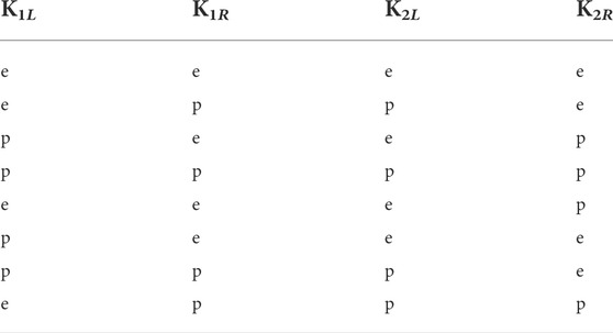
TABLE 1. Eight different cases of two adjoining kink tail configurations. Here, e denotes an exponential tail and p denotes a power law tail (see text for details).
In Sections 3, 4, 5, 7, and 8, we present one-parameter family of potentials where the kink tails have the form mentioned in Table 1 with at least one tail being a power law tail. In addition, in Section 6, we present a one-parameter family of potentials with kink tails of the form ette and pttp, where t, e, and p correspond to power-tower [32], exponential, and power law tail, respectively. For simplicity, we have omitted all inessential factors appearing in these family of potentials. The readers can of course obtain all these factors in the relevant studies cited at appropriate places.
3 Potentials admitting kink and mirror kink solutions with tails of the form e p p e
In this section, we present a one-parameter family of potentials of the form [31].
The potentials for n = 1 and n = 2 with three degenerate minima are depicted in Figure 1 and that for n = 3 and n = 4 in Figure 2. This family of potentials has received wide attention in the literature starting with the 1979 study of Lohe [4], where in the context of massless mesons he introduced this potential for the case of n = 1. The implicit kink solution for n = 1, 2, 3 was first discussed in the study mentioned in reference [1], who pointed out that the kink tail around ϕ = 0 has a power law fall off. In 2019 Manton [23] attacked the nontrivial problem of the calculation of the K-K and the K-AK force for this model in case n = 1; subsequently, this calculation was extended to the entire family [24]. We will discuss the K-K and the K-AK force calculations in detail in Section 10.
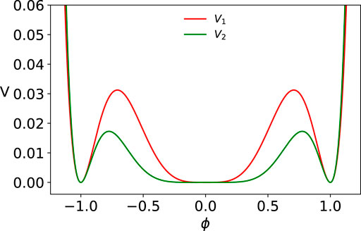
FIGURE 1. Potentials given by Eq. 32 with n = 1 (V1) and n = 2 (V2).
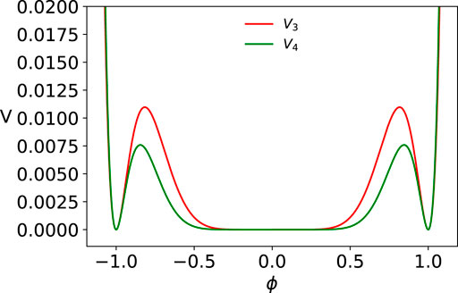
FIGURE 2. Potentials given by Eq. 32 with n = 3 (V3) and n = 4 (V4).
The potential in Eq. 32 for any integer n has degenerate minima at ϕ = 0, ±1 with V(ϕ = 0, ±1) = 0 and admits a kink solution from 0 to 1 and a mirror kink solution from −1 to 0 and the corresponding two antikink solutions with a power law tail around ϕ = 0 and an exponential tail around ϕ = ±1. Unfortunately, in none of these cases, explicit kink solutions can be obtained, and we can only find implicit kink solutions. From the latter, we can obtain how a kink profile falls off as x → ±∞. It turns out that the nature of the implicit kink solution crucially depends on whether n is an odd or an even integer. We, therefore, consider the two cases of odd n = 1 (i.e., potentials of the form ϕ8) and even n = 2 (i.e., potentials of the form ϕ10) separately and then generalize to arbitrary n.
3.1 Case I: n = 1
On using Eq. 7, the self-dual first order equation for the kink solution from ϕ = 0 to ϕ = 1 is:
This is easily integrated with the implicit kink solution.
where A is a constant, which without any loss of generality, we can put equal to zero. It is straightforward to show that in case A = 0, asymptotically,
Thus, the kink tail around ϕ = 0 is entirely determined by the first term on the right hand side of Eq. 34, that is, the term 1/ϕ.
3.2 Case II: n = 2
On using Eq. 7, the self-dual first order equation for the n = 2 case is:
This is easily integrated with the implicit kink solution.
so that, asymptotically,
Thus, the kink tail around ϕ = 0 is again entirely determined by the first term on the right hand side of Eq. 37, that is, the term 1/ϕ2.
Generalization of these results for arbitrary n is straightforward [31], and one finds that for the one-parameter family of potentials, as given by Eq. 32, for arbitrary integer n, while the kink tail falls off like e−2x around ϕ = 1, it falls off like x−1/n around ϕ = 0.
3.3 Kink mass
Using Eq. 9 one can immediately estimate the kink mass for the entire family of potentials as given by Eq. 32. We find that
so that the kink mass decreases as n increases. For example, while MK(n = 1) = 2/15, MK(n = 2) = 1/12. Note that the mass of the kink, mirror kink, and the two antikinks is the same.
4 Potentials admitting kink and mirror kink solutions with tails of the form p e e p
In this section, we present a one-parameter family of potentials of the form [31].
The potentials for n = 1 and n = 2 with three degenerate minima are depicted in Figure 3 and that for n = 3 and n = 4 in Figure 4. Specifically, these potentials have degenerate minima at ϕ = 0, ±1 with V(ϕ = 0, ±1) = 0 and admit a kink from 0 to 1 and a mirror kink from −1 to 0 and corresponding two antikinks. Here, while around ϕ = ±1 one has a power law tail, around ϕ = 0 one has an exponential tail. In these cases too, explicit analytic kink solutions are not possible and we can only find implicit kink solutions. However, from the latter we can determine how the kink profile falls off as x → ±∞.
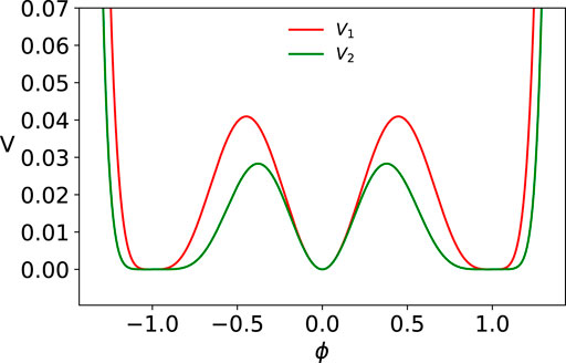
FIGURE 3. Potential given by Eq. 40 with n = 1 (V1) and n = 2 (V2).
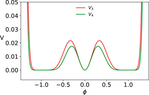
FIGURE 4. Potential given by Eq. 40 with n = 3 (V3) and n = 4 (V4).
We will first discuss the case n = 1 (i.e., the ϕ10 field theory) [1] and n = 2 (i.e., ϕ14 field theory) and then mention the behavior of the kink tail for arbitrary n.
4.1 Case I: n = 1
On using Eq. 7, the self-dual first order equation is:
This is easily integrated with the implicit kink solution.
It then follows that asymptotically:
Thus, the kink tail around ϕ = 1 is entirely determined by the first term on the right hand side of Eq. 42, that is, the term 1/(1 − ϕ2).
4.2 Case II: n = 2
On using Eq. 7, the self-dual first order equation for the n = 2 case is:
This is easily integrated with the implicit kink solution.
Asymptotically,
Thus, the kink tail around ϕ = 1 is again entirely determined by the first term on the right hand side of Eq. 45, that is, the term
Generalization of these results for arbitrary n is straightforward [31], and one finds that for the one-parameter family of potentials, as given by Eq. 40, as x → −∞, the kink tail around ϕ = 0 falls off like ex, whereas as x → +∞, the kink tail around ϕ = 1 falls off like x−1/n.
4.3 Kink mass
Using Eq. 9 one can immediately estimate the kink mass for the entire family of potentials as given by Eq. 40. We find that
Thus, while MK(n = 1) = 1/6, MK(n = 2) = 1/8, that is, the kink mass decreases as n increases.
5 Potentials admitting kink and mirror kink solutions with tails of the form p p p p
In this section, we discuss a two-parameter family of potentials:
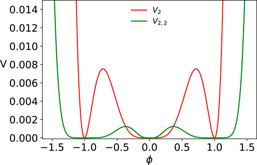
The potentials for three different cases (i) m = n = 1, (ii) m = 1, n = 2, and (iii) m = 2, n = 1 each with three degenerate minima are depicted in Figure 5. Similarly, the potentials for three other cases (iv) m = n = 2, (v) m = 3, n = 2, and (vi) m = 2, n = 3 are depicted in Figure 6. Specifically, these potentials have degenerate minima at ϕ = 0, ±1 and V(ϕ = 0, ±1) = 0 and admit a kink solution from 0 to 1 and a mirror kink solution from −1 to 0 and the corresponding antikink solutions, and all of them have a power law tail at both the ends. We look for a kink solution which goes from 0 to 1 as x goes from − ∞ to +∞, respectively. In these cases too, the explicit analytic solutions are not possible and we can only find implicit kink solutions. From the latter, we can obtain how a kink profile falls off as x → ±∞.
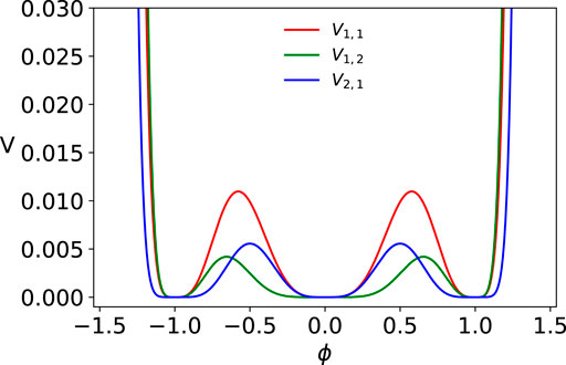
FIGURE 5. Potential given by Eq. 48 with n = m = 1 (V1,1), n = 1 m = 2 (V1,2), and n = 2 and m = 1 (V2,1).
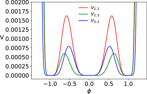
FIGURE 6. Potential given by Eq. 48 with n = m = 2 (V2,2), n = 2 m = 3 (V2,3), and n = 3 and m = 2 (V3,2).
In these models, depending on if m < n (m > n), one can have kink solutions for which the power law tail around ϕ = 1 has slower (faster) asymptotic fall off compared to the power law tail around ϕ = 0 whereas for m = n the power law tails around both ϕ = 0 and ϕ = 1 have similar fall off. As an illustration, we discuss one case each of the three types.
5.1 Models where the kink tail around ϕ = ±1 has a slower asymptotic fall off compared to the tail around ϕ = 0, that is, m < n
For illustration, let us consider the simplest case of m = 1, n = 2 in the potential given by Eq. 48, that is,
On using Eq. 7 the self-dual first order equation is:
This is easily integrated using the identity.
leading to the implicit kink solution
Hence, asymptotically,
Thus, the kink tail around ϕ = 1 is entirely determined by the first term on the right hand side of Eq. 52. On the other hand, the kink tail around ϕ = 0 is entirely determined by the second term on the right hand side of Eq. 52, that is, the term 1/ϕ.
5.2 Models where the kink tail around ϕ = 0 has a slower asymptotic fall off compared to the tail around ϕ = 1, that is, n < m
For illustration, let us consider the simplest case of m = 2, n = 1 in Eq. 48, that is, consider the potential
On using Eq. 7 the self-dual first order equation is:
This is easily integrated leading to the implicit kink solution.
Thus, asymptotically,
Hence, the kink tail around ϕ = 0 is entirely determined by the first term on the right hand side of Eq. 56. On the other hand, the kink tail around ϕ = 1 is entirely determined by the second term on the right hand side of Eq. 56, that is, the term 1/(1 − ϕ2).
5.3 Models where the kink tails around ϕ = 0 and ϕ = 1 have similar asymptotic behavior, that is, m = n
For illustration, let us consider the simplest case of m = 1, n = 1 in Eq. 48, that is, consider the potential
On using Eq. 7 the corresponding first order self-dual equation is:
This is easily integrated using the identity (51) leading to the implicit kink solution.
Thus, asymptotically,
Hence, while the kink tail around ϕ = 1 is entirely determined by the first term on the right hand side of Eq. 60, the kink tail around ϕ = 0 is entirely decided by the second term on the right hand side of Eq. 60, that is, the term 1/ϕ. As expected, in this case the kink tail falls off like x−1 around both ϕ = 1 and ϕ = 0.
Generalization of these results to the most general potential (48) with arbitrary m and n is straightforward and one can show that [31] for the kink solution between 0 and 1 the kink tail asymptotically behaves as x−1/m around ϕ = 0 and as x−1/n around ϕ = 1.
5.4 Kink mass
Using Eq. 9 one can immediately estimate the kink mass for the entire family of potentials as given by Eq. 48. We find that
It is easy to check that the kink mass decreases as either n or m increases.
5.5 Models having a single kink and an antikink with power law tails
Before completing this section it is worth mentioning that the simplest models admitting kink solution with a power law tail at both the ends are:
The potentials with n = 1 and n = 2 are discussed in Section 11 (Eq. 146) and shown there in Figure 10. These models for arbitrary n ≥ 1 admit a kink solution from −1 to 1 and an antikink solution from 1 to −1 with power law tails around both ϕ = ±1. Note that for n = 0 we have the celebrated ϕ4 potential with exponential tails around both ϕ = ±1. Thus, these models for n ≥ 1 are the simplest generalizations of the ϕ4 model but the tail behavior is entirely different than that for the ϕ4 kink. It is also worth noting that unlike the ϕ4 case, for any n ≥ 1, one can only obtain an implicit kink solution from which one can obtain the behavior of the kink tails around both ϕ = ±1. As an illustration, we first discuss the simplest case of n = 1 and then generalize the results for arbitrary n.
5.5.1 Case I: n = 1
On using Eq. 7, the self-dual first order equation is:
This is easily integrated using the identity (51), and we find:
From here, it is straightforward to show that
Note that the leading contribution as x → ±∞ comes from the first term on the right hand side of Eq. 65. The generalization to arbitrary n is now straightforward, and we find that the kink tails around both ϕ = +1 and −1 go like x−1/n.
5.5.2 Kink mass
Using Eq. 9, one can immediately estimate the kink mass for the entire family of potentials as given by Eq. 63. We find that
Note again that the kink mass decreases as n increases.
6 Models with power-tower kink tails
In this section, we consider two different models giving rise to kink solutions with kink tails of the form ette and pttp, respectively. Here, t corresponds to the power-tower type of kink tail, whereas e and p as before correspond to exponential and power law tails, respectively.
6.1 Models with tails of the form ette
Let us consider a one-parameter family of logarithmic potentials of the form [32].
The potential for m = 1 with three degenerate minima is depicted in Figure 7 and for m = 2 in Figure 8. These potentials have degenerate minima at ϕ = 0, ±1 with V(ϕ = 0, ±1) = 0 while they have degenerate maxima at
Thus, notice that while ϕmax(m = 1) = ±e−1/2, as m becomes larger, ϕmax moves toward ±1. On the other hand, while Vmax(m = 1) = 1/8e2, as m becomes larger, Vmax decreases progressively toward zero. All these models for any integer m admit a kink solution from 0 to 1 and a mirror kink solution from −1 to 0 (and the corresponding antikink solutions) with exponential tails around ϕ = ±1 and power-tower tails around ϕ = 0.
For the potential (68) we need to solve the self-dual first order equation
For the kink solution between 0 and 1, we need to solve the self-dual Eq. 70 with negative sign. This is easily integrated by making the substitution t = (1/2) ln(ϕ2) and we obtain the implicit kink solution
where Ei(x) denotes the exponential integral function [41, 42]. Unfortunately, we do not know how to invert this function analytically [43] and obtain t and hence ϕ as a function of x. However, using the Taylor series expansion of Ei(x) [41].
as well as the asymptotic formula [41].
one can estimate the tail behavior around ϕ = 0 as x → −∞ and around ϕ = 1 as x → +∞. Here γ = 0.577 is Euler’s constant. One finds that
It is worth pointing out that the asymptotic behavior around ϕ = 0 (as x → −∞) in Eq. 74 can also be written as follows:
which is known in the literature as the power-tower function of order two [44] or tetration [45].
If one inverts Eq. 74 numerically, one finds that asymptotically as x → −∞, around ϕ = 0 the power-tower tail essentially behaves as a power law tail where the exponent is not known precisely.
6.1.1 Kink mass
One can easily calculate the kink mass for the entire family of potentials. In particular, for the kink potential as given by Eq. 68, the kink mass turns out to be
Observe that even in this case the kink mass decreases as m increases.
6.2 Models with tails of the form pttp
Let us consider a two-parameter family of logarithmic potentials
The potential for m = 1 and n = 1 with three degenerate minima is depicted in Figure 7. Similarly, the potential with m = 2 and n = 2 is depicted in Figure 8. These potentials have degenerate minima at ϕ = 0, ±1 with V(ϕ = 0, ±1) = 0 while they have degenerate maxima at
Notice that both ϕmax and Vmax depend on two parameters m and n. Furthermore, for a fixed m, as n → ∞, ϕmax → 0, and Vmax → ∞. On the other hand, for a fixed n, as m → ∞, ϕmax → 1, and Vmax → 0. Finally, for m = n, ϕmax = ±e−1 and the corresponding Vmax = 1/2e2(n+1). It is interesting to note that for a given m, all the potentials as given by Eq. 77 with arbitrary integer n have the same value
All these models, for any integers m and n admit a kink solution from 0 to 1 and a mirror kink solution from −1 to 0 (and corresponding antikink solutions) with a power law tail around ϕ = ±1 and a power-tower tail around ϕ = 0.
In order to obtain the kink solution from 0 to 1, we need to solve the self-dual equation.
This is easily done by making the substitution t = (1/2) ln(ϕ2), and we obtain [32] the implicit kink solution.
where we need to take + x ( −x) in Eq. 79 depending on whether n is an odd (or even) integer. We then find that
6.2.1 Kink mass
One can easily calculate the kink mass for the entire family of potentials given by Eq. 77, and we find
The kink mass decreases as m increases keeping n fixed. On the other hand, the kink mass increases (decreases) as n increases keeping m fixed depending on the values of m and n. For example, MK(n, m) > ( < ) MK(n + 1, m) depending on if m > ( < ) n + 1.
7 Kink solutions with tails of the form p p p e
We now briefly discuss a one-parameter family of potentials of the form [31].
These potentials have degenerate minima at
7.1 − 1 to 1 kink solution
On using Eq. 7, the self-dual first order equation for the potential (83) is:
This is easily integrated with the solution [31]
Note that in Eq. 85 we have only specified those terms which contribute to the dominant asymptotic behavior as x → ±∞. Asymptotically,
Thus, for the kink solution from −1 to 1, the kink tail around both ϕ = −1 and ϕ = 1 has a power law tail going like x−1/n.
7.1.1 Mass of −1 to 1 kink
It is straightforward to calculate the kink mass for the entire family as given by Eq. 83, and we find that
where B[a, b] is Euler’s beta function [46].
7.2 1 to
On using Eq. 7, the self-dual first order equation is given by
This is easily integrated with the solution
Note that in Eq. 89, we have only specified those terms which contribute to the dominant asymptotic behavior as x → ±∞. Asymptotically,
where h(n) is a known function of n. Thus, for the kink solution from 1 to
7.2.1 Mass of 1 to
It is straightforward to calculate the kink mass for the entire family as given by Eq. 83, and we find that
where 2F1 denotes a hypergeometric function.
8 Kink solutions with tails of the form e e e p
We now briefly discuss a one-parameter family of potentials of the form [31].
These potentials have degenerate minima at
8.1 − 1 to 1 kink solution
On using Eq. 7, the self-dual first order equation for the potential (92) is as follows:
This is easily integrated with the solution [31].
Note that in Eq. 94 we have only specified those terms which contribute to the dominant asymptotic behavior as x → ±∞. Asymptotically, we find that,
where f(n) is a known function of n. Thus for the kink solution from −1 to 1, the kink tail around both ϕ = −1 and ϕ = 1 has an exponential tail.
8.1.1 Mass of −1 to 1 kink
It is straightforward to calculate the kink mass for the entire family as given by Eq. 92, and we find that
8.2 1 to
On using Eq. 7, the self-dual first order equation is now given by
This is easily integrated with the solution [31].
Note that in Eq. 98 we have only specified those terms which contribute to the dominant asymptotic behavior as x → ±∞. Asymptotically,
Thus for the kink solution from 1 to
8.2.1 Mass of 1 to
It is straightforward to calculate the kink mass for the entire family as given by Eq. 92, and we find that
9 Explicit kink solutions with power law tails
In the last six sections, we have presented a number of one-parameter family of potentials wherein one could obtain kink solutions such that at least one of the kink tails has a power law fall off. Unfortunately, in all these cases one could only obtain implicit kink solutions. It is clearly desirable and of interest to look for models where one could obtain kink solutions in an explicit form. That would offer a deeper insight into the various aspects of kink solutions with power law tails. For example, one could then explicitly calculate the kink stability potential, as defined in Section 2 (see Eqs. 15, 16) and verify that for kink solutions with power law tails, indeed there is no gap between the zero mode and the beginning of the continuum, thereby providing a concrete example to the proof given in Section 2. We now discuss three models, two polynomial and one nonpolynomial type, where explicit kink solutions with power law tails can be obtained.
9.1 Model I
We now obtain explicit kink solutions with power law tails in a one-parameter family of potentials characterized by the potential [33].
Note that this potential has degenerate minima at ϕ = 0, ±1 with V(ϕ = 0, ±1) = 0 and admits a kink solution from 0 to 1 and a mirror kink solution from −1 to 0 and the corresponding two antikink solutions. It is worth pointing out that whereas the potential (101) is continuous, its derivative is discontinuous at ϕ = ±1. However, since for the kink as well for the antikink solutions −1 ≤ ϕ ≤ 1, this discontinuity would not matter as far as the kink and the antikink solutions are concerned.
In order to obtain the kink solution from 0 to 1, we need to solve the self-dual equation.
This is easily integrated yielding
It is straightforward to see that
Since the kink solution is explicitly known, the kink stability potential U(x) which appears in the Schrödinger-like Eq. 15 is easily calculated using Eqs. 16 and (104).
As expected, this kink potential U(x) vanishes as x → ±∞ thereby confirming that indeed in this case there is no gap between the zero mode and the beginning of the continuum. Furthermore, one finds that
Using the explicit kink solution (104), it is straightforward to calculate the translation zero mode in the kink stability Schrödinger-like Eq. 15
As expected this zero mode vanishes as x → ±∞, that is, as ϕ → 0, 1.
9.1.1 Kink mass
It is easy to calculate the kink mass in this case. We find
9.2 Model II
Let us consider a one-parameter family of potentials [33].
Note that this potential has degenerate minima at ± 1 with V(ϕ = ±1) = 0 and admits a kink solution from −1 to 1 and the corresponding antikink solution from 1 to −1. Note also that as in the previous example, whereas the potential (109) is continuous, its derivative is discontinuous at x = ±1. However, since for the kink as well as for the antikink solutions −1 ≤ ϕ ≤ 1, this discontinuity would not matter as far as the kink and the antikink solutions are concerned.
In order to obtain the kink solution from −1 to 1, we need to solve the self-dual equation.
This is easily integrated yielding
Eq. 111 is inverted with ease yielding an explicit kink solution.
It is straightforward to see that
It is worth pointing out that for the special case of n = 1, the kink solution (112) has been obtained previously [11].
It is easily checked that, as expected the zero mode eigenfunction vanishes as x → ±∞, that is, as ϕ → ±1. Using the explicit kink solution (112), the kink stability potential U(x) which appears in the Schrödinger-like Eq. 15 is easily calculated.
As expected, this kink stability potential vanishes as x → ±∞, thereby confirming that indeed in this case too there is no gap between the zero mode and the beginning of the continuum.
Using the explicit kink solution (112), it is straightforward to calculate the zero mode and we find
9.2.1 Kink Mass
Finally, it is easy to calculate the kink mass in this case. We find
9.3 Model III
Let us consider the periodic potential [34, 35].
Note that this periodic potential has degenerate minima at ϕ = ±π/2 with V(ϕ = ±π/2) = 0 and admits a kink solution from − π/2 to π/2 and the corresponding antikink solution from π/2 to − π/2. Note that unlike the two previous examples, not only the potential (117) but its derivative is also continuous.
In order to obtain the kink solution from − π/2 to π/2, we need to solve the self-dual equation
This is easily integrated yielding the kink solution
It is straightforward to see that
Using the explicit kink solution (119), the kink stability potential U(x) which appears in the Schrödinger-like Eq. 15 is easily calculated
As expected, this kink stability potential vanishes as x → ±∞ thereby confirming that indeed in this case too there is no gap between the zero mode and the beginning of the continuum. Using the explicit kink solution (119) it is straightforward to calculate the zero mode and we find
9.3.1 Kink Mass
Finally, it is easy to calculate the kink mass in this case. We find
We might add here that apart from the nonpolynomial potential (117) discussed above, a couple of one-parameter family of nonpolynomial models have also been introduced in [3] for which explicit kink solutions have been obtained.
10 Kink–kink and kink–antikink forces
Now we turn to perhaps the most important but not so well understood topic of the calculation of the kink–kink (K-K) and the kink–antikink (K-AK) forces amongst two widely separated kinks with power law tails which are capable of interacting over very large distances. This is in contrast to the well-known ϕ4 and many other kinks with exponential tails for which the calculation of the K-K force between two well separated kinks relies on a linear superposition of the exponentially small tails in the region between the kinks. One then finds that for such kinks the K-K as well as the K-AK forces decay exponentially fast with the kink separation. Furthermore, while the K-K force is repulsive and the K-AK force is attractive, the magnitude of the K-K and the K-AK forces are equal.
On the other hand, for the extended kinks (i.e., kinks with a power law tail), any formula for the force would only make sense to the leading order in the separation even when the separation is large and subleading terms are meaningless. It is worth pointing out that a long time ago Gonzáles and Estrada-Sarlabous [5, 6] had predicted how the force between such a kink and an antikink should decay as a function of the separation between them. However, they did not have a similar prediction for the kink–kink force. Furthermore, they had no specific prediction for the numerical coefficient appearing in the formula. In a remarkable paper, Manton [23] gave a detailed prescription for the calculation of the force between the two well separated kinks and a well separated kink and antikink pair in the case of the potential (discussed in Section 3)
He not only predicted that both the forces should vary as the inverse fourth power of the distance between the two well separated kinks (or the kink and antikink) but more importantly also calculated the pre-factor multiplying this exponent in both the cases and showed that remarkably this factor is very different in the case of K-K and the K-AK forces.
In a subsequent paper, Christov et al. [24] generalized this calculation and estimated the force between two well separated kinks as well as between a kink and an antikink in the one-parameter family of potentials (discussed in Section 3)
They showed that both the K-K and K-AK forces decay like x−2(n+1)/n where x is the distance between the two kinks or between the kink and the antikink thereby reconfirming the prediction of Gonzáles and Estrada-Sarlabous [5, 6]. They also estimated the pre-factor multiplying the exponent and confirmed that this exponent is indeed very different in the case of the K-K and K-AK forces. Furthermore, they compared their predictions with a detailed numerical computation in the specific cases of n = 1, 2, 3. Note that n = 1 is the case studied by Manton while n = 2, 3 correspond to the ϕ10 and ϕ12 models, respectively.
10.1 K-K and K-AK forces for the ϕ8 model
In this review article we will only briefly discuss the key points of the ϕ8 case, the details can be found in [23, 24] as well as in [25, 47]. In [23] Manton has discussed two different approaches for estimating the K-K and K-AK forces and showed that to the leading order, both approaches give a similar answer for the two forces. In the first approach he calculates the force exerted on one kink by using a version of the Noether’s theorem to calculate the rate of change of its momentum [23]. This is equivalent to using the energy-momentum tensor (introduced in Section 2, see Eqs. 3, 4) to estimate the stress exerted on the half line containing the kink. In the second approach he tries to approximately solve the full time-dependent field equations. A simpler but cruder approximation [5, 6] is to just set up a static field configuration that incorporates both kinks, satisfying the appropriate boundary conditions. The nontrivial part in both methods is about the ansatz for the interpolating field.
We would like to remind the readers that as discussed in Section 3, the potential (124) admits a kink solution from ϕ = 0 to ϕ = 1 (which we denote by ϕ0,1(x)), a mirror kink from −1 to 0 (which we denote by ϕ−1,0(x)), an antikink from 1 to 0 (which we denote by ϕ1,0(x)) and a mirror antikink from 0 to −1 (which we denote by ϕ0,−1(x)). Note that while the kink tail around ϕ = 0 has a fall off like x−1, the kink tail around ϕ = ±1 has an exponential fall off. Manton in his paper [23] has calculated the force between the mirror kink ϕ−1,0(x) and the kink ϕ0,1(x). He has also calculated the force between the antikink ϕ1,0(x) and the kink ϕ0,1(x). As shown in Section 3, the kink energy (i.e., mass) in this case is 2/15 (see Eq. 39). Furthermore, the implicit kink solution ϕ0,1(x) as given by Eq. 34 is
where A can be thought of as the position of the kink. From here it is straightforward to obtain the asymptotic behavior
Now if ϕ(x − A) is the kink solution then the mirror kink solution can be shown to be − ϕ( − x − A). This is because both the kink and the mirror kink obey the same Bogomolnyi Eq. 34.
Let us assume that the kink is located at A and mirror kink at − A with A ≫ 0. Let us now split the spatial line at − X and X with 0 ≪ x ≪ A so that for x < − X we have an exact mirror kink field and for x > X we have an exact kink field. For the intermediate region − X < x < X one assumes that the interpolating field has a linear behavior that is, ϕ(x) = μx which leads to X = A/2 and μ = 4/A2. It is then straightforward to calculate the kink energy to leading order in 1/A and one finds the repulsive force between the kink and the mirror kink to be (note the force is the negative derivative of the energy with respect to the separation of the kink and the mirror kink) [23]
This calculation is conceptually easy to follow and gives expected dependence of F on A although the coefficient 32/5 is not so accurate. Proceeding in the same way, and assuming that a well separated kink is located at A and an antikink at − A, Manton goes on to calculate the attractive force between the kink and the antikink. One assumes that the field is symmetric in x at all times. Furthermore, he splits up the spatial line at + A/2 and − A/2 so that for x ≤ −A/2 one has an exact antikink field while for x ≥ A/2 one has an exact kink field. In between − A/2 ≤ x ≤ A/2, the interpolating field is assumed to have quadratic behavior, that is, ϕ(x) = α + βx2 where α and β are determined by demanding that ϕ(x) is continuous and has continuous first derivative at x = ±A/2. One finds α = 1/A, β = 4/A3. It is then straightforward to calculate the kink–antikink energy to the leading order in 1/A and the attractive force between the kink and the antikink turns out to be [23].
Manton then goes on to use an alternative approach [23] where he models the kink by a field of the form
The acceleration is then
Thus the profile ξ(y) satisfies a static equation which depends on the acceleration a and evolves adiabatically with time as a varies. Manton assumes that a varies slowly with time and the effect of the term aξ′(y) is to change the effective potential to
On integrating it from ξ = 0 to ξ = ∞ this yields the acceleration [23]
and hence the K-K force is
Note that this number is different from the estimate obtained in Eq. 128 by using the static field approach. Manton has provided justification as to why this number is more reliable than that given by Eq. 128.
By using a similar approach Manton has also calculated the attractive interaction between the ϕ1,0(x) antikink and the ϕ0,1 kink. The only difference is that since the kink and the antikink attract, hence unlike the K-K case, now
On integrating ξ(y) from ξ = (4a/15)1/4 to ξ = ∞ one then obtains the acceleration and hence the corresponding K-AK force [23]
One thus finds that unlike the exponential tail case (where the magnitude of the K-K and K-AK forces are equal), for the power law kinks of the ϕ8 model (124), the ratio of the magnitude of the K-AK and K-K force is about 1/4. This is rather remarkable and one needs to understand why this is so.
10.2 K-K and K-AK forces for the family of potential (125)
There are several obvious ϕ8 questions. The first question is how good is this theoretical prediction? Secondly, can one extend it to the entire one-parameter family of potentials given by Eq. 125? These questions have been answered by Christov et al. [24] by extending the Manton calculation to the entire family of potentials (125). They show that for the K-K case one again obtains Eq. 132 except one has to replace ξ4(y) by ξ2n+2(y) and replace the kink mass 2/15 by 2/(n + 2)(n + 4) (see Eq. 39). One then finds that the K-K force for the entire family of potentials (125) is given by
The corresponding K-AK force is similarly obtained with the same replacement as above in Eq. 135 and one finds [24]
As expected, for n = 1 one retrieves the Manton results for the K-K and the K-AK force as given by Eqs. (134) and (136), respectively. Furthermore, on using the well known identities
it is straightforward to show that [24]
Thus as n increases, the tail becomes progressively longer, that is, as we go from ϕ8 to ϕ10, ϕ12 and higher order models, one finds that that the K-AK force becomes progressively weaker compared to the corresponding K-K force and whereas this ratio is −1/4 for n = 1, this ratio goes to zero in the limit n → ∞. It is worth remembering that for the exponential kink tails, the two forces are always equal and opposite. This is a highly nontrivial result which needs a deeper understanding.
These theoretical predictions have been compared with the detailed numerical simulations for the n = 1, 2, 3 cases (i.e., ϕ8, ϕ10 and ϕ12) in [24] (also see [25]). There are major challenges in even initializing kinks with a power law tail numerically. There is a concern that the initial conditions in a direct numerical simulation of interactions may substantially affect the nature of the observed interactions [26]. On using the split-domain ansatz and periodic boundary conditions, numerically accurate predictions were obtained for the K-K and the K-AK forces in case n = 1, 2 and 3. They find that while the agreement for the exponent is excellent for all the three cases, the agreement about the pre-factor multiplying the exponent is excellent for the ϕ8 case (as given by Eqs. (134) and (136)), but as n increases to 2 and 3, the agreement about the pre-factor gradually becomes worse. One of the reasons for this disagreement is that as n increases, the kink tail becomes progressively longer.
Can we extend the above calculations in case the kink tails are of the form peep or pppp or ette or pttp or pppe or eeep? We now show that the answer is yes and give predictions for the K-K and K-AK forces in the above cases when the two tails facing each other have a power law fall off.
10.3 Predictions for FK−AK in the case of peep
Let us consider the one-parameter family of potentials as given by Eq. 40, that is,
This model admits a kink ϕ0,1(x), a mirror kink ϕ−1,0(x) with an exponential tail around ϕ = 0 and a power law tail around ϕ = ±1. It also admits an antikink ϕ1,0(x) and a mirror antikink ϕ0,−1(x).
Following the procedure discussed above, it is straightforward to calculate the force between the kink ϕ0,1(x) and the antikink ϕ1,0(x). The two differences compared to the eppe case discussed above are (1) in this case in the long-range limit the potential around ϕ = 1 is
This is rather remarkable and suggests that the K-K and K-AK forces are independent of the kink mass and only depend on the asymptotic behavior of the power law kink tail. Let us now check if the same is borne out in case the tails are of the form pppp.
10.4 Predictions for FK-K and FK−AK in the case of pppp
Let us consider the one-parameter family of potentials as given by Eq. 48, that is,
This model admits a kink ϕ0,1(x), a mirror kink ϕ−1,0(x) with a power law tail around ϕ = 0 as well as around ϕ = ±1. It also admits an antikink ϕ1,0(x) and a mirror antikink ϕ0,−1(x). In particular, while the tail around ϕ = 0 asymptotically goes like x−1/m, the power law tails around ϕ = ±1 go like x−1/n.
Following the procedure discussed above, it is straightforward to calculate the force between the mirror kink ϕ−1,0(x) and the kink ϕ0,1(x) as well as the force between the antikink ϕ1,0(x) and the kink ϕ0,1(x) by noting that in this case the potential around ϕ = 0 is given by
In this model one can also calculate the force between the kink ϕ0,1(x) and the antikink ϕ1,0(x) since the kink tail around ϕ = 1 also has a power law tail. On noting that in the long-range limit the potential around ϕ = 0 is given by
Finally we come to the question of the K-K and K-AK forces in the model with power-tower kink tails as discussed in Section 6. As has been discussed in detail in [32], the power-tower tails essentially are power law tails varying like x−1/a with a being a real positive number. We would like to remark that the calculation of [24] which is valid when the kink tail goes like x−1/n where n is an integer, is easily extended to the case where the tail falls off like x−1/a and a is a real positive number. In particular, the expressions for the K-K force, the K-AK force and their ratio continue to be still given by Eqs. (137), (138) and (140) with the obvious replacement of n by a. As has been shown in [32], for potentials
where the kink tails are of the form ette, the kink tail around ϕ = 0 falls off like x−1/a where 0 < a < 1 and as m increases the value of a decreases progressively. It appears that these potentials may provide a bridge between the kink solutions with a power law tail and the kink solutions with an exponential tail. It would be highly desirable to understand this transition.
Proceeding in the same way, it is straightforward to compute the K-K and K-AK forces and their ratio in the case of other models discussed in this review.
11 Kink–antikink collisions at finite velocity
The issue of kink–antikink (K-AK) collisions at finite velocity is only recently being addressed in the context of the kinks with a power law tail [26–29]. Before we discuss the results obtained, nontrivial issues involved and some of the open problems, it is worth pointing out that in the context of kinks with an exponential tail, the K-AK collisions at finite velocity have been extensively discussed during the last four and half decades [48, 49, 50, 50a, 50b, 50c, 51, 51a, 52, 53, 53a, 53b, 53c, 53d, 53e, 54, 54a, 54b, 55, 56, 57, 57a, 58, 59, 60, 61, 62]. However, it is fair to say that a coherent physical explanation is still lacking. Some of the key findings are the following.
1) There is a critical value vcr of the initial velocity which is model dependent but typically of the order of 0.1 − 0.3 (in units of c, the speed of light) separating two different regimes of collision: for vin < vcr, the capture and the formation of a bound state occurs, while for vin > vcr, the kink and the antikink escape to infinity after a single collision.
2) For vin < vcr, besides the formation of a bound state one finds that there are two-bounce, three-bounce and so on escape windows. In particular, there are intervals of the initial velocities within which kinks scatter and eventually escape to spatial infinities. The difference from vin > vcr, however, is that inside the escape windows the kinks scatter to infinity not after a single impact, but even after two or more successive collisions. The escape windows seem to form a fractal structure.
3) The explanation of the escape windows phenomenon seems to vary from model to model. For those models (like ϕ4) where the kink stability equation admits an extra mode called the vibrational mode (i.e., over and above the translational zero mode which is present in every kink bearing model), it has been suggested that the above phenomenon occurs due to the resonant energy exchange between the zero mode and the vibrational mode [62].
4) On the other hand, models where the kink stability equation does not have any vibrational mode (like the celebrated ϕ6 model with
During the last few years researchers have inquired [26–29] if similar behavior also occurs in the collision of power law kinks at finite velocity. The major challenge in case the kinks facing each other having a power law tail is the correct formulation of the initial conditions since the power law kink tails overlap significantly at any finite distance that can be considered as asymptotically large, that is, large enough so that the kink and the antikink could be considered noninteracting. Using the split-domain ansatz [28] the authors have investigated kink–antikink collisions with finite velocity in the ϕ8, ϕ10 and ϕ12 models as given by Eq. 32 with n = 1, 2, 3, that is,
In these models there is a kink from 0 to 1, a mirror kink from −1 to 0 and the corresponding two antikinks with a power law kink tail around ϕ = 0 and an exponential tail around ϕ = ±1. These authors have considered collisions between the kink ϕ−1,0(x) and the antikink ϕ0,−1(x) moving at finite velocity. In all these models they again find the same qualitative behavior as in the collision of the kink and the antikink with an exponential tail. In particular, they again find that there is a critical velocity vcr such that for vin > vcr the kinks escape to infinity after one impact while for vin < vcr there is formation of a kink–antikink bound state. In addition to that, they again find two-bounce, three-bounce and so on escape windows as depicted in Figure 9. The critical velocity vcr monotonically increases from vcr of about 0.15 for the ϕ8 case to about 0.21 for the ϕ10 and to 0.27 for the ϕ12 case.
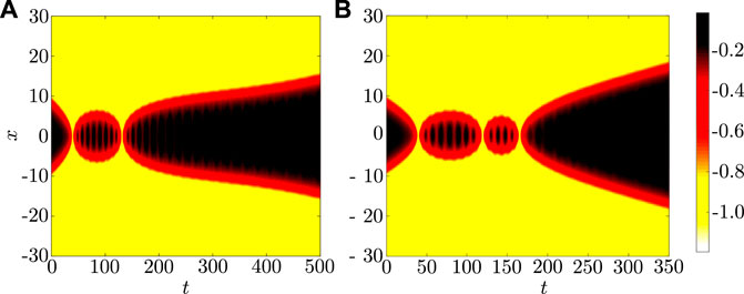
FIGURE 9. Space-time contour plot of the scalar field of the kink–antikink interaction in the ϕ8 model showing (A) two-bounce and (B) three-bounce windows. Adapted from [28].
For the power law kinks, this area of research is in its infancy and hopefully in coming years we will have a better understanding and eventually a coherent physical explanation might be available. Some of the open problems are the following.
1) For the models as given by Eq. 32, for large n do we still have a similar picture as for n = 1, 2, 3? In particular as n becomes progressively larger, does vcr become progressively larger and approach 1 (in units of c, the speed of light) asymptotically? For large values of vcr, how important are the relativistic effects? Of course this a difficult problem since as n increases the kink tails become progressively longer.
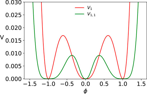
2) The question of vcr being very large is not a hypothetical question because of a recent study [29] of K-AK collisions at finite velocity for different ϕ8,12 models as given by Eq. 63 with n = 1, 2 (see Figure 10), that is,
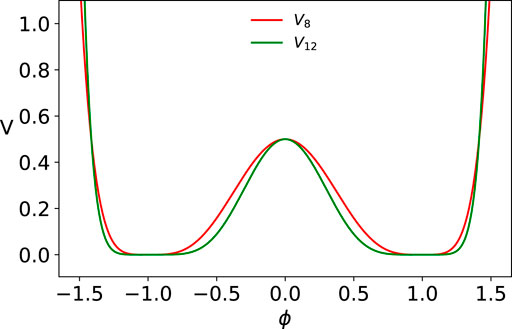
FIGURE 10. ϕ8 (V8) and ϕ12 (V12) potentials given by Eq. 146.
Note that in these models there is only a single kink from −1 to +1 and a corresponding antikink and unlike the model studied by [28], in these models one has a symmetric power law kink tail around ϕ = 1 and ϕ = −1. Using what they term as computationally efficient way, it has been claimed by the authors of [29] that the K-AK collisions at finite velocity behave very differently from all the models studied previously (either with an exponential or a power law tail). In particular, they claim that there is neither a long-lived bound state formation nor resonance windows and vcr is ultrarelativistic. These claims, if true, would indicate that for power law kink tails, the K-AK collisions at finite velocity are conceptually very different from the exponential tail case.
3) Apart from the two possible kind of models studied so far [28, 29], there are several other models with power law kink tails as discussed in Sections 4–9 and one also needs to study K-AK collisions at finite velocity in these models and try to understand various facets of this challenging as well as difficult problem.
Finally, we note that recently kink scattering in a generalized Wess–Zumino model [64] with three minima has been studied, wherein two different scattering channels have been identified, namely, kink–kink reflection and kink–kink hybridization.
12 Open problems
In this review we have tried to uncover various aspects of kink solutions with a power law tail. Several issues are now fairly clear. For example, one distinctive feature of kinks with a power law tail is that the corresponding kink stability equation only admits the translation zero mode and in these cases the beginning of the continuum coincides with the zero mode (i.e., with ω2 = 0). Secondly, there is a recipe available for constructing two adjoining kink solutions with various possible combinations of the power law and the exponential kink tails. In addition, a wide class of kink solutions has been constructed with two of the tails being of power-tower type [32] which is a kind of power law tail behaving like x−1/a where a is any arbitrary positive number. However, there are several aspects of the kink solutions with the power law tail which are either only partially understood or not understood at all. We now list some of these issues.
1) So far only implicit kink solutions with a power law tail have been constructed in models with polynomial potentials. While explicit kink solutions with a power law tail have been constructed in a few models with polynomial potentials, however unfortunately in all these models, while the kink potential V(ϕ) is continuous but its derivative is not. Even though that has still allowed the explicit construction of the kink solutions with a power law tail, it is certainly desirable to obtain kink solutions with a power law tail in models with polynomial potentials where not only the kink potential but its derivative is also continuous everywhere.
2) One of the major issues which is only partially understood is that of the K-K and K-AK forces in the case of the power law tail. In case the kink tails are of the form eppe, one of the intriguing conclusions [23, 24] is that compared to the kink–kink force, the kink–antikink force gets progressively weaker as the kink tail becomes progressively longer. This is in contrast to the kinks with exponential tails for which the magnitudes of the K-K and K-AK forces are always equal. In our view, understanding the reason for the weak K-AK force compared to the K-K force remains one of the major open problems.
3) The calculation of [24] for the K-K and K-AK forces is only reliable for smaller values of n in the family of potentials given by Eq. 125 since as n increases, the kink tails become progressively longer. It is highly desirable to devise methods for a reliable computation of the K-K and K-AK forces for the entire family of potentials as given by Eq. 125.
4) Are the results derived by [23, 24] for the eppe case for the K-K and K-AK forces and their ratio also valid for the other kink tail configurations such as peep and pppp (with suitable modification for the form of the potential in the asymptotic limit and the corresponding kink mass)? In Section 10, we have assumed this to be true and tried to make predictions for the K-K and K-AK forces and their ratio in the other cases with power law kink tails. How good are these predictions? It would be desirable if these could be checked by accurate numerical calculations.
5) The predictions for the K-K and K-AK forces have been made in [23, 24] for the eppe case, which indicated that the kink tail goes like x−1/n where n is any integer. Are these results also valid in case the kink tail goes like x−1/a with a being any positive number? In Section 10, we have assumed it to be true and tried to make predictions for the K-K and K-AK forces in case the kink tails are of the form ette or pttp and on the basis of these predictions have suggested that the power-tower kink tails [32] form a bridge between the exponential and the power law tails. How good are these predictions? It would be desirable if these could also be checked by accurate numerical calculations.
6) The predictions made in [23, 24] for the K-K and K-AK forces are only valid to the leading order and only for the large separation between the two kinks or the kink and the antikink. Is it possible to compute the subleading corrections to these estimates?
7) In all the calculations an implicit assumption has been made that these results do not depend on the effect of the two (of the four) tails which are not facing each other. While it may be a reasonable assumption in the eppe case where the other two tails are exponential, it is not obvious if it is also true in case the kink tails are of the form pppp. It would be highly desirable if one can numerically check the validity of this prediction.
8) Normally for exponential tails, the K-K and K-AK forces fall off exponentially as a function of the distance between them. Is this conclusion still valid if the two remaining kink tails have a power law fall off as in the peep case?
9) Can one extend the calculation of Manton [23] to the case of nonpolynomial models [3, 34, 35] with a power law kink tail? Knowing the behavior of the power law kink tail, one can perhaps predict how the K-K and K-AK forces fall off as a function of the kink–kink (or kink–antikink) separation. However, it is not at all obvious how to compute the pre-factor multiplying it using the Manton approach [23].
10) There are several areas of physics where kink solutions with a power law tail could have applications. However, to date we do not have any such concrete examples. Finding a concrete example will give an added motivation for an in-depth study of kinks with power law tails.
11) Very little is known about the kink–antikink collisions at finite velocity in the case of kinks with power law tails. In fact, one has conflicting results about such collisions for the eppe case [28] compared to the case where there is a single kink with symmetric power law kink tails at both the ends [29]. It is clearly important to study such collisions in other models discussed in Sections 4–9 where too one has kink solutions with a power law tail.
12) Recently we have also constructed models having super-exponential (se) [40] and super-super-exponential (sse) [65] kink tails. It may be of interest to enquire if one can construct models where the two adjoining kinks have an arbitrary combination of the power law, the exponential, the super-exponential and the super-super-exponential tails.
13) Several years ago Bazeia et al. [66] proposed a novel deformation function
We hope that in the coming years insightful answers would be obtained for at least some of the questions raised above, further enriching the field of power law kink tails.
Author contributions
AK and AS authors conceptualized the problem, calculated, discussed, wrote and edited the manuscript.
Acknowledgments
We thank Ayhan Duzgun for help with the figures. AK is grateful to the Indian National Science Academy (INSA) for the award of the INSA Senior Scientist position at Savitribai Phule Pune University, Pune, India. The work at Los Alamos National Laboratory was carried out under the auspices of the U.S. DOE and NNSA under contract no. DEAC52-06NA25396.
Conflict of interest
The authors declare that the research was conducted in the absence of any commercial or financial relationships that could be construed as a potential conflict of interest.
Publisher’s note
All claims expressed in this article are solely those of the authors and do not necessarily represent those of their affiliated organizations, or those of the publisher, the editors, and the reviewers. Any product that may be evaluated in this article, or claim that may be made by its manufacturer, is not guaranteed or endorsed by the publisher.
References
1. Khare A, Christov IC, Saxena A. Successive phase transitions and kink solutions in ϕ8, ϕ10, and ϕ12 field theories. Phys Rev E (2014) 90:023208. doi:10.1103/PhysRevE.90.023208
2. Saxena A, Christov IC, Khare A. Higher-order field theories: ϕ6, ϕ8 and beyond. In: PG Kevrekidis, and J Cuevas-Maraver, editors. A dynamical perspective on the ϕ4 model: Past, present and future. Springer (2018).
3. Bazeia D, Menezes R, Moreira DC. Analytical study of kinklike structures with polynomial tails. J Phys Commun (2018) 2:055019. doi:10.1088/2399-6528/aac3cd
4. Lohe MA. Soliton structures in P(var ϕ)2. Phys Rev D (1979) 20:3120–30. doi:10.1103/physrevd.20.3120
5. González JA, Holyst JA. Solitary waves in one-dimensional damped systems. Phys Rev B (1987) 35:3643–6. doi:10.1103/physrevb.35.3643
6. González JA, Estrada-Sarlabous J. Kinks in systems with degenerate critical points. Phys Lett A (1989) 140:189. doi:10.1016/0375-9601(89)90891-8
7. Mello BA, González JA, Guerrero LE, Lopez-Atencio E. Topological defects with long-range interactions. Phys Lett A (1998) 244:277–84. doi:10.1016/s0375-9601(98)00213-8
8. Guerrero LE, González JA. Long-range interacting solitons: Pattern formation and nonextensive thermostatistics. Physica A: Stat Mech its Appl (1998) 257:390–4. doi:10.1016/s0378-4371(98)00165-4
9. Guerrero LE, López-Atencio E, González JA. Long-range self-affine correlations in a random soliton gas. Phys Rev E (1997) 55:7691–5. doi:10.1103/physreve.55.7691
10. Bazeia D, González León MA, Losano L, Mateos Guilarte J. Deformed defects for scalar fields with polynomial interactions. Phys Lett (2006) 73:105008. doi:10.1103/PhysRevD.73.105008
10a. Bazeia D, González León MA, Losano L, Mateos Guilarte J. New scalar field models and their defect solutions. Euro Phys Lett (2011) 93:41001. doi:10.1209/0295-5075/93/41001
11. Gomes AR, Menezes R, Oliveira JCRE. Highly interactive kink solutions. Phys Rev D (2012) 86:025008. doi:10.1103/physrevd.86.025008
12. Radomskiy RV, Mrozovskaya EV, Gani VA, Christov IC. Topological defects with power-law tails. J Phys : Conf Ser (2017) 798:012087. doi:10.1088/1742-6596/798/1/012087
13. Rajaraman R. Introduction to solitons and instantons. North Holland: North-Holland Publishing Company (1973).
15. Vilenkin A, Shellard EPS. Cosmic strings and other topological defects. Cambridge, UK: Cambridge University Press (2001).
16. Vachaspati T. Kinks and domain walls: An introduction to classical and quantum solitons. Cambridge, UK: Cambridge University Press (2006).
17. Shnir YM. Topological and nontopological solitons in scalar field theories. Cambridge, UK: Cambridge University Press (2018).
19. Gufan YM, Larin ES. Phenomenological consideration of the isostructural phase transition. Dokl Akad Nauk SSSR (1978) 242:1311.
20. Pavlov SV, Akimov ML. Phenomenological theory of isomorphous phase transitions. Crystall Rep (1999) 44:297.
21. Boulbitch AA. Crystallization of proteins accompanied by formation of a cylindrical surface. Phys Rev E (1997) 56:3395–400. doi:10.1103/physreve.56.3395
22. Greenwood E, Halstead E, Poltis R, Stojkovic D. Electroweak vacua, collider phenomenology, and possible connection with dark energy. Phys Rev D (2009) 79:103003. doi:10.1103/physrevd.79.103003
23. Manton NS. Forces between kinks and antikinks with long-range tails. J Phys A: Math Theor (2019) 52:065401. doi:10.1088/1751-8121/aaf9d1
24. Christov IC, Decker R, Demirkaya A, Gani VA, Kevrekidis PG, Khare A, Saxena A. Kink-kink and kink-antikink interactions with long-range tails. Phys Rev Lett (2019) 122:171601. doi:10.1103/physrevlett.122.171601
25. Christov IC, Decker RJ, Demirkaya A, Gani VA, Kevrekidis PG, Radomskiy RV. Long-range interactions of kinks. Phys Rev D (2019) 99:016010. doi:10.1103/physrevd.99.016010
26. Belendryasova E, Gani VA. Scattering of the φ8 kinks with power-law asymptotics. Commun Nonlinear Sci Numer Simul (2019) 67:414–26. doi:10.1016/j.cnsns.2018.07.030
27. Gani VA. Vibrations of thick domain walls: How to avoid no-go theorem. J Phys : Conf Ser (2020) 1690:012095. doi:10.1088/1742-6596/1690/1/012095
28. Christov IC, Decker RJ, Demirkaya A, Gani VA, Kevrekidis PG, Saxena A. Kink-antikink collisions and multi-bounce resonance windows in higher-order field theories. Commun Nonlinear Sci Numer Simul (2021) 97:105748. doi:10.1016/j.cnsns.2021.105748
29. Campos JGA, Mohammadi A. Interaction between kinks and antikinks with double long-range tails. Phys Lett B (2021) 818:136361. doi:10.1016/j.physletb.2021.136361
30. Manton NS. An effective Lagrangian for solitons. Nucl Phys B (1979) 150:397–412. doi:10.1016/0550-3213(79)90309-2
31. Khare A, Saxena A. Family of potentials with power law kink tails. J Phys A: Math Theor (2019) 52:365401. doi:10.1088/1751-8121/ab30fd
32. Khare A, Saxena A. Wide class of logarithmic potentials with power-tower kink tails. J Phys A: Math Theor (2020) 53:315201. doi:10.1088/1751-8121/ab84ac
33. Khare A, Duzgun A, Saxena A. Explicit kink solutions in several one-parameter families of higher-order field theory models. Int J Mod Phys B (2021) 35:2150324. doi:10.1142/s0217979221503240
34. Mohammadi M, Riazi N, Azizi A. Radiative properties of kinks in the sin4(ϕ) system. Prog Theor Phys (2012) 128:615–27. doi:10.1143/ptp.128.615
35. Kulagin DA, Omeĺyanov GA. Asymptotics of kink-kink interaction for sine-gordon type equations. Math Notes (2004) 75:63. doi:10.1023/B:MATN.0000023337.12918.c8
35a. Omeĺyanov GA, Segundo-Caballero I. Asymptotic and numerical description of the kink/antikink interaction. Electron J Diff Equ (2010) 2010:1.
37. Cooper F, Khare A, Sukhatme UP. Supersymmetry in quantum mechanics. Phys Rep (1995) 251:267. doi:10.1016/0370-1573(94)00080-M
38. Christ NH, Lee TD. Quantum expansion of soliton solutions. Phys Rev D (1975) 12:1606–27. doi:10.1103/physrevd.12.1606
39. Landau LD, Lifshitz EM. Quantum mechanics: Non-relativistic theory, course of theoretical physics vol. 3. 3rd ed. London: Pergamon Press (1977).
40. Kumar P, Khare A, Saxena A. A minimal nonlinearity logarithmic potential: Kinks with super-exponential profiles. Int J Mod Phys B (2021) 35:2150114. doi:10.1142/s0217979221501149
41. Harris FE. Table of contents for issues of mathematical tables and other aids to computation. Math Tables Other Aids Comput (1957) 11(57):9–16.
42. Gradshteyn IS, Ryzhik IM. Table of integrals, series and products. 7th ed. Boston: Academic Press (2007).
43. Pecina P. On the function inverse to the exponential integral function. Bull Astron Inst Czechosl (1986) 37:8.
44.Wolfram. Wolfram MathWorld (2022). Available at: http://mathworld.wolfram.com/PowerTower.html.
45.Tetration. Tetration (2022). Available at: https://en.wikipedia.org/wiki/Tetration.
46. Abramowitz M, Stegun IA. Handbook of mathematical functions. Mineola, NY: Dover Publishng (1964).
47. Peru d’Ornellas J. Forces between kinks in ϕ8 theory. J Phys Commun (2020) 4:055014. doi:10.1088/2399-6528/ab90c2
49. Sugiyama T. Kink-antikink collisions in the two-dimensional ϕ4 model. Prog Theor Phys (1979) 61:1550–63. doi:10.1143/ptp.61.1550
50. Campbell DK, Schonfeld JF, Wingate CA. Resonance structure in kink-antikink interactions in φ4 theory. Physica D: Nonlinear Phenomena (1983) 9:1–32. doi:10.1016/0167-2789(83)90289-0
50a. Peyrard M, Campbell DK. Kink-antikink interactions in a modified sine-Gordon model. Physica D (1983) 9:33.
50c. Campbell DK, Peyrard M, Sodano P. Kink-antikink interactions in the double sine-Gordon equation. Physica D (1986) 19:165.
51. Goodman RH, Haberman R. Kink-antikink collisions in the phi^4 equation: The n-bounce resonance and the separatrix map. SIAM J Appl Dyn Syst (2005) 4:1195–228. doi:10.1137/050632981
51a. Goodman RH, Rahman A, Bellanich MJ, Morrison CN. A mechanical analog of the two-bounce resonance of solitary waves: Modeling and experiment. Chaos (2015) 25:043109.
52. Belova TI, Kudryavtsev AE. Solitons and their interactions in classical field theory. Phys -Usp (1997) 40:359–86. doi:10.1070/pu1997v040n04abeh000227
53. Gani VA, Kudryavstev AE. Kink-antikink interactions in the double sine-Gordon equation and the problem of resonance frequencies. Phys Rev E (1999) 60:3305–9. doi:10.1103/physreve.60.3305
53a. Gani VA, Moradi Marjaneh A, Askari A, Belendryasova E, Saadatmand D. Scattering of the double sine-Gordon kinks. Eur Phys J C (2018) 78:345.
53b. Bazeia D, Belendryasova E, Gani VA. Scattering of kinks of the sinh-deformed φ4 model. Eur Phys J C (2018) 78:340.
53c. Moradi Marjaneh A, Gani VA, Saadatmand D, Dimitriev SV, Javidan K. Multi-kink collisions in the ϕ6 model. JHEP (2017) 2017:28.
53d. Gani VA, Moradi Marjaneh A, Saadatmand D. Multi-kink scattering in the double sine-Gordon model. Eur J Phys C (2019) 79:620.
53e. Moradi Marjaneh A, Askari A, Saadatmand D, Dimitriev SV. Extreme values of elastic strain and energy in sine-Gordon multi-kink collisions. Eur Phys J B (2017) 91:22.
54. Baziea D, Gomes AR, Nobrega KZ, Simas FC. Oscillons in hyperbolic models. Phys Lett B (2020) 803:135291.
54a. Baziea D, Gomes AR, Nobrega KZ, Simas FC. Kink scattering in hyperbolic models. Int J Mod Phys A (2019) 34:1950200.
54b. Bazeia D, Gomes AR, Simas FC. Semi-compactness and multiple oscillating pulses in kink scattering. Eur Phys J C (2021) 81:532.
55. Alonso-Izquierdo A, Quiero-Nunes J, Nieto LM. Scattering between wobbling kinks. Phys Rev D (2021) 103:045003. doi:10.1103/physrevd.103.045003
56. Mohammadi N, Dehghani R. Kink-antikink collisions in the periodic φ4 model. Commun Nonlinear Sci Numer Simul (2021) 94:105575. doi:10.1016/j.cnsns.2020.105575
57. Adam C, Oles K, Romaǹczukiewicz T, Wereszczynski A. Kink-antikink scattering in the ϕ4 model without static intersoliton forces. Phys Rev D (2020) 101:105021. doi:10.1103/physrevd.101.105021
57a. Adam C, Oles K, Romaǹczukiewicz T, Wereszczynski A. Kink-antikink collisions in a weakly interacting ϕ4 model. Phys Rev D (2020) 102:062214.
59. Yan H, Zhong Y, Liu Y-X, Maeda K-I. Kink-antikink collision in a Lorentz-violating ϕ4 model. Phys Lett B (2020) 807:135542. doi:10.1016/j.physletb.2020.135542
60. Manton NS, Oles K, Romaǹczukiewicz T, Wereszczynski A. Kink moduli spaces: Collective coordinates reconsidered. Phys Rev D (2021) 103:025024.
61. Pereira CFS, Luchini G, Tassis T, Constantinidis CP. Some novel considerations about the collective coordinates approximation for the scattering of ϕ 4 kinks. J Phys A: Math Theor (2021) 54:075701. doi:10.1088/1751-8121/abd815
62. Lizunova M, van Wezel J. An introduction to kinks in φ4-theory. Scipost Phys Lect Notes (2021) 23.
63. Dorey P, Mersh K, Romaǹczukiewicz T, Shnir Y. Kink-antikink collisions in the ϕ6 model. Phys Rev Lett (2011) 107:091602. doi:10.1103/physrevlett.107.091602
64. Alonso-Izquierdo A, González León MA, Martin Vaquero J, de la Torre Mayado M. Kink scattering in a generalized Wess-Zumino model. Commun Nonlinear Sci Numer Simul (2021) 103:106011.
65. Khare A, Saxena A. Logarithmic potential with super-super-exponential kink profiles and tails. Phys Scr (2020) 95:075205. doi:10.1088/1402-4896/ab8eeb
66. Bazeia D, Losano L, Malbouisson JMC. Deformed defects. Phys Rev D (2002) 66:101701. doi:10.1103/physrevd.66.101701
67. Almeida CL, Bazeia D, Losano L, Malbouisson JMC. New results for deformed defects. Phys Rev D (2004) 69:067702. doi:10.1103/physrevd.69.067702
68. Bazeia D, Losano L. Deformed defects with applications to braneworlds. Phys Rev D (2006) 73:025016. doi:10.1103/physrevd.73.025016
69. Blinov PA, Gani TV, Gani VA. Domain wall thickness and deformations of the field model. J Phys : Conf Ser (2020) 1690:012085. doi:10.1088/1742-6596/1690/1/012085
71. Bazeia D, Belendryasova E, Gani VA. Scattering of kinks of the sinh-deformed var ϕ4 model. Eur Phys J C (2018) 78:340. doi:10.1140/epjc/s10052-018-5815-z
Keywords: kink tails, power law tails, kink collisions, stability analysis, higher order field theories, power-tower tail, kink-kink and kink-antikink forces
Citation: Khare A and Saxena A (2022) Kink solutions with power law tails. Front. Phys. 10:992915. doi: 10.3389/fphy.2022.992915
Received: 13 July 2022; Accepted: 05 September 2022;
Published: 30 September 2022.
Edited by:
Luigi Fortuna, University of Catania, ItalyReviewed by:
Roberto Zivieri, University of Trento, ItalyNicholas Manton, University of Cambridge, United Kingdom
Copyright © 2022 Khare and Saxena. This is an open-access article distributed under the terms of the Creative Commons Attribution License (CC BY). The use, distribution or reproduction in other forums is permitted, provided the original author(s) and the copyright owner(s) are credited and that the original publication in this journal is cited, in accordance with accepted academic practice. No use, distribution or reproduction is permitted which does not comply with these terms.
*Correspondence: Avadh Saxena, YXZhZGhAbGFubC5nb3Y=