Success of social inequality measures in predicting critical or failure points in some models of physical systems

Statistical physicists and social scientists both extensively study some characteristic features of the unequal distributions of energy, cluster, or avalanche sizes and of income, wealth, etc., among the particles (or sites) and population, respectively. While physicists concentrate on the self-similar (fractal) structure (and the characteristic exponents) of the largest (percolating) cluster or avalanche, social scientists study the inequality indices such as Gini and Kolkata, given by the non-linearity of the Lorenz function representing the cumulative fraction of the wealth possessed by different fractions of the population. Here, using results from earlier publications and some new numerical and analytical results, we reviewed how the above-mentioned social inequality indices, when extracted from the unequal distributions of energy (in kinetic exchange models), cluster sizes (in percolation models), or avalanche sizes (in self-organized critical or fiber bundle models) can help in a major way in providing precursor signals for an approaching critical point or imminent failure point. Extensive numerical and some analytical results have been discussed.

1 Introduction

Unequal distributions of resources (e.g., income or wealth) among the population are ubiquitous. Economists, in particular, quantify such inequalities in distributions using some inequality indices (e.g., Gini and Kolkata), defined through the Lorenz function [1, 2] ([3], for recent review). Unequal distributions of energy (per degrees of freedom), of cluster sizes (sites and bonds), or of avalanches (elements failing in one go) in many-body systems are also ubiquitous and also extensively studied in various physical systems by statistical physicists over the ages ([4–6]). Physicists usually concentrate on the (fractal) structure of the biggest (in size) cluster or avalanche, which becomes of the order of the system size, inducing the eventual macroscopic self-similarity and the consequent critical behavior characterized by the critical exponents ([5, 6]).

Economists traditionally quantify the social inequalities in distributions using inequality indices, defined through the Lorenz function L(f) [7]. After ordering the population from the poorest to the richest, the Lorenz function L(f) is given by the cumulative wealth fraction possessed by the fraction f of the population, starting from the poorest: L (0) = 0 and L (1) = 1 (Figure 1). If everyone had an equal share of the wealth, L(f) = f would be linear (called the equality line), and the old and still most popular inequality index, namely the Gini (g) index [8], is given by the area between the equality line and the Lorenz curve, normalized by the entire area (1/2) below the equality line. Thus, g = 0 corresponds to perfect equality, and g = 1 corresponds to extreme inequality. Another recently introduced inequality index, namely, the Kolkata (k) index [9], can be defined as the nontrivial fixed point of the complementary Lorenz function L_c(f) ≡ 1 − L(f): L_c(k) = k. It says that the richest (1 − k) fraction of the population possesses a fraction k of the total wealth (k = 1/2 corresponds to perfect equality and k = 1 corresponds to extreme inequality). As such, the k index quantifies and generalizes the century old 80–20 law (corresponding to k = 0.80) of Pareto [10]. Extensive analysis of social data ([11, 12]) indicates that in extremely competitive situations, the indices k and g become equal in magnitude of about 0.86 (instead of 0.80).

FIGURE 1

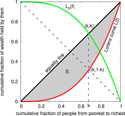
FIGURE 1. Lorenz curve L (f) (shown in red) and complementary Lorenz curve L_c (f) (shown in green) used to calculate the inequality indices Gini (g = 2S, S denoting the area of the shaded region between the equality line and the Lorenz curve) and Kolkata (given by the fixed point k = L_c (k) ≡ 1 − L(k)). Here, L represents the cumulative fraction of wealth possessed by p fraction of the people, when ordered from poorest to the richest. For the physical systems considered here, such as the kinetic exchange model of gas, the wealth could be replaced by the kinetic energy and the fraction of people by the fraction of particles. For model systems such as percolation, sandpiles, or the fiber bundles, the horizontal axis represents the fraction (f) of clusters or avalanches when all avalanches are arranged from the lowest to the highest size. The vertical axis (L) represents the fraction of the cumulative mass of these clusters or avalanches.

The Gibbs distribution ([4]) of kinetic energy among the particles in a classical ideal gas in equilibrium can also be analyzed in terms of the corresponding Lorenz function $L\left(\right.(f)$ and then extracting the Gini (g) and Kolkata (k) indices for the kinetic exchange models of market by exploiting the formal similarity between the energy of the gas molecules in the kinetic theory and wealth of an individual and that between temperature and noise in trade ([13–15]). Similarly, the distributions of cluster sizes ([6]) in the percolation models on lattices can be analyzed in terms of the g and k indices. At occupation concentration p both below and above the percolation threshold p_c ≃ 0.5927 [6] gave g = k ≃ 0.865 at a site occupation probability p ≃ 0.565, somewhat below the percolation threshold p_c. The statistics of avalanches (successive failures in one go, without any increase in the external perturbation), following the self-organizing critical dynamics of the sand-pile models ([16]) have also recently been analyzed in terms of the behavior of social inequality indices g and k [17]. Finally, the avalanche statistics due to collective dynamics of failure or breaking of individual elements (in non-brittle materials), studied using the fiber bundle models (FBMs) ([18–21]), when analyzed using the social inequality indices g and k [17, 22], gives an intriguing possibility of predicting the imminent failure of the entire bundle.

Typical FBMs or such failure-prone (dynamically coupled many-element) systems, or the percolating systems, are not self-organized and are externally driven or tuned. Particularly for the FBM, a discrete set of elements, each having a failure threshold randomly drawn from a distribution, carries a load. The elements are irreversibly broken when the load on them cross the pre-assigned threshold value. Either the remaining intact elements (fibers) are able to support the applied load, or at a sufficiently high value of the applied load (the critical load for the system), the entire system breaks down. Unlike the other cases discussed here, there are no dynamics on the other side of the critical point, as the system does not survive at all beyond the critical load. For self-organized-critical (SOC) systems, ([16]), as the average “height” h per site increases, our numerical study (in square lattice) [17] shows that g and k approach each other and become equal to about 0.863 (BTW), and 0.856 (Manna) at the respective values of average heights h ≃ 2.087 (little less than the actual critical value h_c = 17/8 = 2.125) for the BTW model and h ≃ 0.6859 (compared to h_c ≃ 0.7172) for the Manna model. For the other SOC models considered here [17, 22], such as the driven-interface Edwards–Wilkinson model and the centrally pulled FBM, show similar growth (from g = 0 and k = 0.5) of the inequality indices to about g = k ≃ 0.86 a little below the respective SOC points.

All these numerical studies indicate that, except for the irreversible dynamical systems such as FBMs (where the dynamics eventually stop), all critical systems (self-organized or otherwise) show a clear precursor behavior of the inequality indices such as the Gini g and Kolkata k. Particularly, if the inequality in the response of a physical system is measured as it approaches a critical point, such measures show universal trends, irrespective of the universality class of the associated critical point. The particular response to be measured depends on the particular system. For example, in the case of site percolation, it is the inequality between the clusters for a given occupation probability; for kinetic exchange model of wealth, it is the wealth distribution between the individuals; for SOC systems, it is the time series of the avalanches. The inequality indices Gini (g) and Kolkata (k) typically start from 0 to 0.5 respectively (for small and almost equal size clusters), when the systems are far away from the critical point. Then, they approach g = k ≃ 0.86 slightly before the critical point is reached. Even for irreversible systems such as the FBMs, the indices g and k assume universal terminal values of about 0.45 and 0.65, respectively, providing a major statistical precursor signal for the impending catastrophes.

Here, we reviewed some recent numerical studies on the properties of Gini (g) and Kolkata (k) indices for extended kinetic exchange models [14], with some analytical Landau-like formulation of the Lorenz function L(f) and the analytical estimates of g and k and the relationships between them, including an estimate of the self-organized poverty (energy) level. Next, discussed the numerical observations on g and k for site percolating systems in two dimensions and discussed, in particular, how their coincidence in magnitude (g = k ≃ 0.86) occurs preceding the imminent percolation or critical point. Similar results [17] (g = k ≃ 0.86) as the sandpile systems approach the self-organized critical point in the Bak–Tang–Wiesenfeld sandpile model, Manna model, and a centrally pulled self-organized fiber bundle model have been discussed. Finally, have discussed the numerical results (g ≃ 0.45 and k ≃ 0.65) as the global breaking point approach [22, 23] in the equal-load-sharing fiber bundle models with irreversible local failures and collective load-share mechanism and their relevance in earthquake statistics [24].

2 Numerical results for social inequality indices in kinetic exchange, percolation, BTW, Manna, and fiber bundle models

In this section, we have mostly discussed numerical results for the Gini [3, 8] and Kolkata [3, 9] indices for the kinetic exchange models [13, 25, 26], percolating systems [6, 27] and three self-organized-critical (SOC) models, namely, the Bak–Tang–Wiesenfeld model (BTW) [28], Manna model [29], and a self-organizing centrally-pulled-fiber-bundle model [18, 19]. We also discussed the same for the standard fiber bundle model (FBM) [30] ([19–21]), where the irreversible breaking dynamics stop as the whole bundle fails. Except for the kinetic exchange model considered here, all the other models exhibit critical, externally tuned (as in percolation), or self-organized (as in BTW, Manna, or centrally pulled fiber bundle) behavior at (in percolation model) or beyond (for the SOC models) the respective critical points (traditionally identified as the phase transition point). The bundle failure points (stress) in such FBMs have already been identified as the corresponding critical points [19–21, 31].

As mentioned earlier, statistical physicists have studied extensively, over the last five decades, the building up of self-similarity in the spatial and temporal structures of the clusters or avalanches near the critical point, where the system spanning cluster (corresponding to the divergent correlation length [4–6]) or the consequent critically slow dynamics (divergent relaxation time [4–6]), characterized by the (singular and universal) exponents, occur. This self-similar system-spanning fractal structure developed at the critical point is necessarily very much unequal compared to the other structures, which become quite unimportant there. The Lorenz function [7] of these cluster or avalanche size distributions near these critical points are found to become such that the Gini (g) and Kolkata (k) indices become equal and nearly universal (g = k ≃ 0.86 or becomes nearly universal (g ≃ 0.45, k ≃ 0.65) at the breaking or failure points of FBMs. This equality (g = k ≃ 0.86) or otherwise (g ≃ 0.45, k ≃ 0.65) is seen to follow from Monte Carlo data in various model cases discussed in this section, and it occurs a little away from the critical point where the inequalities become much larger. This universal value of the inequality indices in various physical systems, prior to the arrival of the respective (widely different) critical points, can provide excellent precursor signals.

2.1 Social indices g and k in kinetic exchange models

First, we recount in brief the derivation of energy (ϵ) distribution n (ϵ), representing the number of constituent free (Newtonian) particles of a classical ideal gas in equilibrium at a temperature T. If g (ϵ) denotes the “density of states”, giving g (ϵ)dϵ equal to the number of dynamical states possible for any of the free particles of the gas which has kinetic energy between ϵ and ϵ + dϵ (as counted by the different momentum vectors $\vec{p}$ corresponding to the same kinetic energy ϵ ∼|p|² (giving $g(ϵ)dϵ\sim \sqrt{ϵ}dϵ$ in three dimension); then, one can write n (ϵ)dϵ = g (ϵ)ρ(ϵ, T) dϵ. For completely stochastic and ergodic many-body dynamics or energy conserving exchanges, the statistical energy distribution function ρ (ϵ, T) should satisfy ρ(ϵ₁)ρ (ϵ₂) = ρ (ϵ₁ + ϵ₂) for any arbitrary choice of ϵ₁ and ϵ₂. This suggests ρ (ϵ) ∼ exp (−ϵ/T). These finally give $n(ϵ)=\sqrt{ϵ}\exp (ϵ/T)$, where the factor T can be identified from the observed knowledge about the equation of state for the gas.

In a natural extension of this oldest and most established many-body theory, econophysicists developed ([13, 25]) the Kinetic exchange model of trading markets with fixed total money (M = N) exchanged only among fixed (large) number (N) agents or traders. Here, the money m_i(t) [M = ∑_im_i (t)] at any time t (measured by the number of trades or scattering) of the i-th agent (or “social atom”) is identified as the kinetic energy (ϵ) of the corresponding atom or particle. In the market, the total amount of money (M = N) remains conserved as no one can print money or destroy money (will end up in jail in both cases). Following the kinetic theory picture of random kinetic energy exchanges among the particles in an ideal gas, the money exchanges among the agents in the market here are considered to be completely random. One would, therefore, again expect, for any buyer–seller transaction in the market, $\rho (m_1)\rho \left(\right.(m{2)=}_{\left.\right)}\rho (m_1+m_2)$, where ρ (m) denotes the equilibrium or steady state distribution of money m among the traders in the market. This, in turn, in a similar way, suggests ρ (m) = A exp (−m/Δ), where A and Δ are constants. Since ∫ρ (m)dm = N = M = ∫mρ (m) dm, we finally get n (m) = ρ (m) = exp (−m) for the steady state number of traders with money m in the market (since there cannot be any equivalent of the particle momentum vector for the agents, the equivalent of the density of states g (m) here is a constant).

1) One can easily calculate [14] exactly both the inequality indices g and k here. We can now calculate the Lorenz function $L(f)={\int }_0^{m}x\rho (x)dx=1-(m+1)exp(-m)$, where $f={\int }_0^m\rho (x)dx=1-exp(-m)$, giving m = − ln (1 − f), giving, in turn, L(f) = 1 − (1 − f)[1 − ln (1 − f)]. One, thus, gets (Figure 1, noting the area under the equality line to be 1/2), the Gini index $g=1-2{\int }_0^{1}L(x)dx=1/2$ and the Kolkata index k given by the self-consistent equation 1 − k = L(k) or 1 − 2k = (1 − k)[ln (1 − k)], giving k ≃ 0.68.

2) We now proceed to study numerically the uniform saving exchange model and the corresponding Gini and Kolkata indices. In this model (called CC model [13, 32, 33]), we consider again a closed economic system with a fixed amount of money M and a fixed number of agents N = M, where the agents are interacting (trading with) each other by exchanging their money. A saving propensity λ(0 ≤ λ ≤ 1) of the agents is introduced in this model, such that during each (two-body) trade event, each of the agents saves a fraction λ of their money in possession at that point of time (trade) and the rest of money is again exchanged randomly between the two trade partners. The exchange of money m_i (t) between two traders (i and j) at time t can be expressed as

$m_i\left(t+1\right)=\lambda m_i\left(t\right)+{ϵ}_{ij}\left(1-\lambda \right)\left(m_i\left(t\right)+m_j\left(t\right)\right),(\mathrm{1a})$

$m_j\left(t+1\right)=\lambda m_j\left(t\right)+{ϵ}_{ij}\left(1-\lambda \right)\left(m_i\left(t\right)+m_j\left(t\right)\right),(\mathrm{1b})$

3) We now proceed with an approximate expansion [15] of the Lorenz function L(p), employing a Landau-like argument [4] for the expansion of free energy. A Landau-type minimal expansion of the Lorenz function L(f) up to the quadratic term f gives

$L\left(f\right)=Af+B{f}^2,A>0,B>0,A+B=1.(2)$

As may be noted, the abovestated expansion gives L (0) = 0 and L (1) = 1, and with the linear term alone, the Lorenz function can represent only the equality line (Figure 1). One can now calculate the Gini index $g=1-2{\int }_0^{1}L(f)df$ giving A = 1 − 3 g and B = 3g. The value of the k index can be found from the relation (Figure 1) L(k) = 1 − k, giving 3gk² + (2 − 3g)k − 1 = 0, or

$k=\frac{\left(3g-2\right)\pm \sqrt{{\left(2-3g\right)}^2+12g}}{6g}.(3)$

In the g → 0 limit, the above expression gives [15] k = 1/2 + (3/8)g, which suggests k = g = 0.8, the Pareto value under extreme competition [10] (see Figure 2). Of course, the full relation Eq. (3) gives g = k ≃ 0.74, which is much smaller than the observed values around 0.86 [3, 12] and even the Pareto value 0.80 (corresponding to Pareto’s 80–20 law [10]).

4) We now discuss the self-organized appearance of minimum energy or poverty level [14] in the kinetic exchange model and in its extension with uniform saving propensity, namely in the CC model. Specifically, we consider a kinetic exchange model where one of the agents in the chosen pair is necessarily the poorest (in money or energy) at that point of time (trade or scattering), and the other one is randomly chosen from the rest. Here, we vary the saving propensity (λ) for values other than 0, and the exchange of money follows the same rule as described by Eq. 3. An important observation is the spontaneous appearance of a self-organized poverty (or energy) level (SOPL) in the steady state distribution, below which the distribution function vanishes (ρ (m) = 0). For λ = 0 the SOPL occurs at m = θ (λ = 0) ≃ 0.61 (Figures 3 and 4). This SOPL [θ (λ)] also increases with increasing values of λ (Figure 3), and the θ(λ) approaches unity as λ approaches unity (Figure 4).

5) We now sketch a mean field-like argument to estimate the value of θ, the self-organized poverty (energy) level (SOPL). If we assume, following Ref. [14], that generally the steady state distribution ρ (m) of money or energy in such kinetic exchange models of SOPL remains Gibbs-like (exponentially decaying, but with shifted origin to m = θ: ρ (m) = exp [ − (m − θ)] for m > θ and ρ (m) = 0 otherwise), the average energy of any of the traders or particles will be equal to [θ + (θ + 1)e⁻¹]/2, which has to be greater than θ. This is because one of the trade partners must have (with probability 1) θ amount of money, while the other can be any one else and can be assumed to have an average money (M/N = 1, shifted by the minimum θ) and, hence, comes with a probability exp (−1). Finally, there will be, on average, a 50–50 share for any one, and that share value has to be equal to or above the minimum (θ). This gives the estimate θ ≤ [θ + (1 + θ)e⁻¹]/2 or θ ≤ e⁻¹/(1 − e⁻¹), giving θ ≤ 0.58. This upper bound is somewhat less than the observed value (Figure 3; θ(0) ≃ 0.61) at λ = 0. For λ approaching unity, the distribution any way approaches equality (at m = 1) [13, 14]. Hence, the abovementioned equation simplifies to θ ≤ [θ + 1]/2, or θ ≤ 1, which is clearly observed.

FIGURE 2

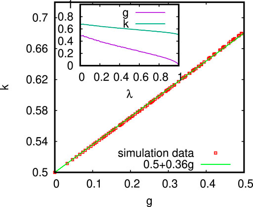
FIGURE 2. Variation of the Kolkata index (k) against the Gini index (g) for kinetic exchange model with uniform saving propensity (λ; CC model). For λ = 0, the estimated values of k ≃ 0.68 and g ≃ 0.5 conform the theoretically estimated exact values of g = 0.5 and k ≃ 0.682, discussed earlier. As expected, with increasing saving propensity, the inequality decreases and g tends to vanish, and k approaches 0.5 as λ tends towards unity. The simulation data fit well with the relation k = 0.5 + Cg with C ≃ 0.36 (a Landau-like theory for the Lorenz function, discussed next, gives C = 3/8). Inset shows the variations of g and k with λ.

FIGURE 3

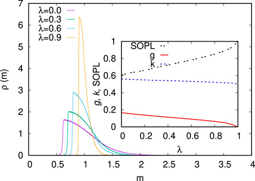
FIGURE 3. Steady state money distribution ρ (m) for fixed saving propensity λ in the kinetic exchange model where in each two-body scattering (trade), one particle (trader) is with least energy (money), and the other one is chosen randomly from the rest. In the inset, the variations of inequality indices k and g and location of the self-organized minimum energy (poverty) level (SOPL) are shown against fixed saving propensity λ. Adapted from [14].

FIGURE 4

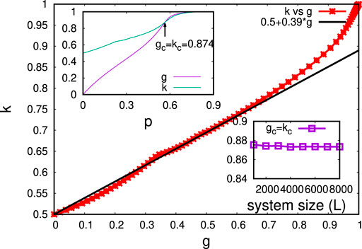
FIGURE 4. Kolkata index (k) against Gini index (g) for 2-d site percolation on square lattice. The initial slope of the simulation data fits well with the relation k = 0.5 + 0.39 g. The upper inset shows the variations of g and k with occupancy probability p, and the crossing value k_c or g_c of k and g is about 0.874 and occurs at p ≃ 0.565, somewhat below p_c ≃ 0.593.

2.2 Social indices g and k in percolation model

In percolation models, a regular square lattice (L × L) with site occupation probability p is considered. The cluster size distribution is measured for different p values. The cluster size s measures the number of the nearest neighbor occupying sites and the number n (s) of s size cluster at any particular p will give the cluster size distribution (at any p), which has been utilized to generate the Lorenz function. The inequality indices g and k are obtained from the Lorenz function (Figure 1) for distributed cluster sizes. Figure 4 shows the variation of the Kolkata index (k) against the Gini index (g) of the cluster sizes for different site occupation probability p (we performed the simulations for system size 4000 × 4000). The initial slope of the simulation data fits well with the relation k = 0.5 + C*g (C ≃ 0.39). The upper inset shows the variation of g and k with occupation probability p and the crossing value of the two indices k_c = g_c ≃ 0.874 at p ≃ 0.565 (while the critical point is p_c ≃ 0.593). The lower inset shows the variation k_c or g_c with system size (L).

2.3 Social indices g and k in Bak–Tang–Wiesenfeld, Manna sandpile, and centrally pulled fiber bundle models

2 3.1 Inequality in the Bak–Tang–Wiesenfeld and Manna sandpile models

In the BTW model on a square lattice, the sand grains are added one by one at randomly selected sites. The heights of the sand columns at different sizes will increase with the addition of these sand grains. When the sand column height (h) at any site reaches a threshold value (4, in the BTW model), the column becomes unstable, and the sand grains from the unstable sites are equally shared among the neighboring (4) sites uniformly. This may cause the neighboring columns to become unstable, and the avalanche continues. In the Manna sandpile model (on square lattice again), when the sand column height reaches a threshold value of 2, the column becomes unstable, and the sand grains from the unstable column are shared randomly by two of the neighboring columns which may become unstable again, and the avalanche may continue. Therefore, an avalanche of topplings will occur in both the models until height h at all the lattice sites becomes less than the respective threshold values. The random addition of sand grains to the sandpile then induces further dynamics in the models. The avalanche size s measures the total number of toppings in one go, without any further addition of sand grain to the system, and the number of s size avalanches n (s) in the steady state of the models will give respective avalanche size distributions, which have been utilized to generate the respective Lorenz functions.

The inequality indices (g and k) are obtained from the abovementioned Lorenz functions for the respective models. Figures 5A B show the variations of the Kolkata index against the Gini index for different average heights of the sand columns in the BTW and Manna models, respectively. The initial variations of the simulation data in both the models seem to fit well with the relation k = 0.5 + C*g (C = 0.385 ± 0.005) and g_c = k_c = 0.860 ± 0.005 for the crossing point. It may be mentioned that this crossing of g and k occurs at the values of average height h ≃ 2.087 (slightly below the actual critical height h_c = 17/8 for the BTW model) and at h = 0.6859 (compared to the actual critical height h_c ≃ 0.7172 for the Manna model) [17]. For a finite size scaling behavior of these values, see Figure 6.

FIGURE 5

FIGURE 5. Kolkata index k against Gini index g plotted for (A) BTW model and (B) Manna model. The initial slope of the simulation data fits well with the relation k = 0.5 + C*g (C = 0.385 ± 0.005) and g_c = k_c = 0.860 ± 0.005 is the crossing point with the g = k line. Taken from Ref. [20].

FIGURE 6

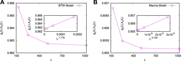
FIGURE 6. (A) BTW sandpile model: The values of the Kolkata k_c(L) and the Gini g_c(L) indices (at the point when they cross) have been plotted as a function of the system sizes L = 128, 256, 512, and 1024. The crossing point (g = k = g_c = k_c) values of the indices decrease with the system size. (Inset) The values of k_c = g_c as a function of L have been extrapolated with respect to L^−1/ν, where the value of ν for the BTW model has been tuned for the best possible linear fit of the data, and it gives 1/ν = 1.776, giving, in turn, k_c = g_c = 0.863 in the limit of L → ∞. (B) Manna sandpile model: The values of the Kolkata index k_c(L) and the Gini index g_c(L) have been plotted against the system sizes L = 128, 256, 512, and 1024. The values of the indices decrease with the system size. (Inset) The values of k_c = g_c as a function of L have been extrapolated with respect to L^−1/ν, and the value of the exponent ν has been tuned for the best possible fit of the data. The plot shows that the best fit corresponds to 1/ν = 2.162 for the Manna model, giving, in turn, k_c = g_c = 0.8554 in the limit of L → ∞. Adapted from Ref. [20].

2.3.2 Inequality in centrally pulled fiber bundle model

In this version of the fiber bundle model [18], initially, a load is applied only at a centrally located fiber in a two-dimensional arrangement of fibers. The applied load (pull) is slowly increased at a constant rate. When that fiber breaks, the load is shared equally between its nearest neighbors. Should some of those neighbors fail, their load would be equally redistributed among all fibers that have at least one broken neighbor. The redistribution process occurs at a much faster rate than the pulling. Hence, the load per fiber value along the centrally located damage boundary fluctuates around a steady state. The numbers of fiber broken in an avalanche show power-law size distribution. Unlike the usual version of the fiber bundle, where the dynamics eventually stop due to a catastrophic failure of the whole system, in this case, it continues until the damage boundary reaches the system boundary, i.e., in the thermodynamic limit of infinite system size, the dynamics keep on going.

The inequality of the avalanches could be measured in the same way as in the case of the SOC models mentioned above. The plots of g vs. k are shown in Figure 7.

FIGURE 7

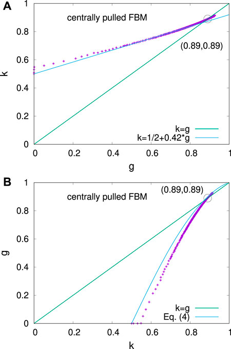
FIGURE 7. Variations of k against g indices are shown for the centrally pulled fiber bundle model. (A) The line is a fit for the initial growth of g and k, while the g = k line is also shown as a guide to the eye. Adapted from Ref. [20]. (B) The same variation is plotted with g against k and compared with Eq. 4.

For a theoretical understanding of this behavior, if the Lorenz function is written as L (f) = f^θ, then, it is known that g = (θ − 1)/(θ + 1). In other words, then, θ = (1 + g)/(1 − g). Now, one gets k from solving 1 − k = k^θ Then, clearly,

$g=\frac{ln\left(1-k\right)-ln\left(k\right)}{ln\left(1-k\right)+ln\left(k\right)}.(4)$

This relation does not restrict the values of g and k and should be valid as long as the form of the Lorenz function is a power-law. It can be compared with the numerical observation of the relation between g and k in the SOC models (discussed later). If, however, one concentrates in the limit of small values of g and k, i.e., k = 1/2 + ϵ, where ϵ → 0, then the above relation reduces to

$k=\frac{1}{2}+\frac{ln\left(2\right)}{2}g.(5)$

The relation Eq. 4 is compared with the simulation of centrally loaded FBM in Figure 7.

2.4 Social indices g and k in the fiber bundle model

In the previous sub Section 2.3 (b), we considered a self-organized version of the fiber bundle model, where the breaking dynamics continue indefinitely as the active fiber bundle system (on the periphery of the central broken patch) grows continuously in size as the central pull or load is increasing with time.

In the standard version of the fiber bundle model ([19–21]), of course, the breaking dynamics stop as the entire stem (fixed in size) fails. Here, the collective dynamics of failure or breaking in any non-brittle material sample proceed through the failures of individual elements of the material as the external load or stress on the sample increases. The subsequent redistribution of the load shares among the surviving elements and consequent further failures and avalanches (even when the external load does not increase any further). These bursts of elastic energy released (experimentally detected as acoustic emissions) until the complete breakdown of the material are widely studied [13]. These bursts or avalanches are also studied often in models, such as the fiber bundle model (FBM) [14, 15], both analytically and numerically. An avalanche is defined as the size or mass of the failure events taking place in the system in going from one stable state to the next, as the external load on the system is increased further to trigger a failure activity (load gradually increased), while the (relatively faster) internal dynamics continues due to load redistribution among the surviving fibers and consequent failures due to such increased load on them. The avalanche size could also be measured by the amount of elastic energy released from these failed elements. Its distribution would then correspond more naturally to the elastic energy emissions. In the mean-field version of the model considered here, these two quantities (avalanche and energy) have the same size distribution function. For simplicity, here, we consider the avalanche size to be given only by the number of failed elements. For successive increases in the external load, further avalanches of different sizes occur with various frequencies. As in the wealth distributions, the distributions of the avalanche sizes across a broad class of systems show the common feature of having a relatively larger number of smaller events (poorer people) and much fewer number of large ones (richer people), indicating similar nonlinear nature of the corresponding Lorenz function L(f) (Figure 1). In statistical physics, however, we usually concentrate on the (fractal) structure, the biggest avalanche size, which becomes of the order of the system size and causes the eventual macroscopic failure of the sample ([5, 6]). Some recent studies [17, 22] on the social inequality indices in equal-load-sharing FBMs [19–21] having widely different fiber breaking threshold distributions, suggest gradual increase of the Gini and Kolkata indices (see Figures 8-10) with increasing load on the bundles, towards some universal terminal values, namely g ≃ 0.45 and k ≃ 0.65, respectively, at the breaking point σ_c (breaking load per fiber) of the respective bundles (see Figure 11). Needless to mention, monitoring the values of such (social) indices g and k for failure avalanches (usually measured as acoustic emissions) can, therefore, provide an easy and unique precursor signal [17, 22] to imminent disasters.

FIGURE 8

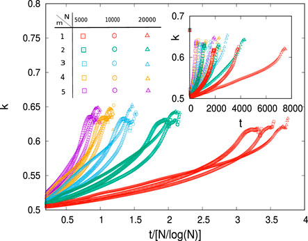
FIGURE 8. Kolkata index k for the avalanche distribution D(Δ) as the dynamics of failure continues in the FBM (in the ELS scheme), where the individual fiber thresholds are drawn from a Weibull distribution. The estimated values of the index k at different times t (scaled by N/log N) are plotted until complete failure of the bundle (with disorder characterized by different Weibull moduli (m) indicated using different colors). The terminal value of the k-index, prior to complete failure bundle, seems to reach a threshold (0.62 ± 0.03), and this terminal value is weakly dependent on m. The inset shows the variations of the k index with unscaled time. Taken from [22].

FIGURE 9

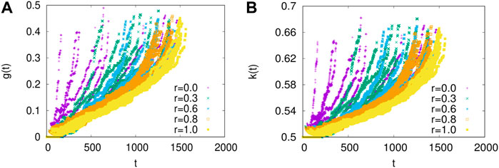
FIGURE 9. Time variations of (A) g(t) and (B) k(t) are shown when individual samples are of sizes between L_min and L_max with uniform probability, where r = L_min/L_max and 10 time series are shown for each value of r. While the failure times for the individual samples are vastly different, the terminal values of g = g_f and k = k_f are narrowly distributed. The failure thresholds are taken from a Weibull distribution with a shape parameter value κ = 3 and L_max = 10,000. Adapted from [23].

FIGURE 10

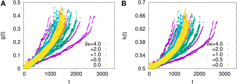
FIGURE 10. The time variations of (A) g(t) and (B) k(t) are shown when individual samples are of different disorder strengths—Weibull threshold distributions with shape parameters distributed uniformly between κ_min and κ_max, with 10 samples for each κ_min, κ_max pair. In the labels, δκ = κ_max − κ_min, with (κ_max + κ_min)/2 = 3.0, in each case. The system size is 1000 always. Again, the failure times are vastly different, but the terminal values of g = g_f and k = k_f are narrowly distributed. Adapted from [23].

FIGURE 11

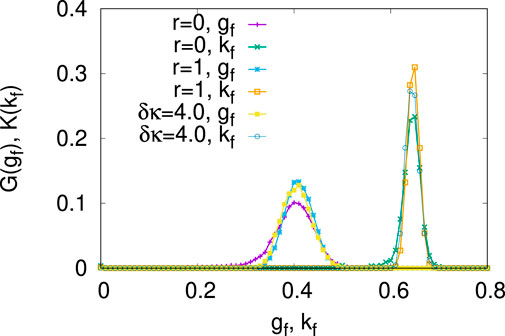
FIGURE 11. Probability distributions of the terminal values of g = g_f (denoted by G (g_f)) and k = k_f (denoted by K (k_f)) are shown for extreme values of r = L_min/L_max = 0, 1 and δκ = 4.0. The distributions show peak near ⟨g_f⟩ = 0.41 ± 0.04 and ⟨k_f⟩ = 0.64 ± 0.02. The averages are calculated over 10,000 ensembles. Adapted from [23].

Indeed, our recent analysis [24] of USGS earthquake magnitude data for 22 years (2000–21) shows universal social inequality indices terminal values. For the fiber bundle model, an analytical estimate of the failure point values of g and k for particular limits (equally spaced failure thresholds and equal load increase) can be attempted [24]. It can give an idea of why the limiting values are independent of the different threshold distributions.

3 Summary and discussion

Many physical systems close to their critical points exhibit large fluctuations. Despite many differences, large groups of systems show universal nature in the statistical features of such fluctuations. In other words, such differences are irrelevant in the renormalization group sense, and the critical points are characterized by sets of critical exponents that only depend on a few subtle parameters (space dimension and order-parameter dimension). Nevertheless, in measuring the critical exponents, the critical points need to be known, which can depend on many details of the particular system under investigation. There can also be some situations where the system can only be probed from one side of the critical point (e.g., breakdown of driven disordered solids). In such cases, knowledge of the proximity to the critical point (imminent breakdown) is often crucial. Knowing some typical universal values of the critical exponents alone does not help in determining the proximity to the critical point.

Here, we have outlined, in a variety of physical systems, how the characterization of the (social) inequality in the response statistics of systems close to the critical points can help in determining the proximity to such a point. It is remarkable that the precursor signal for the forthcoming transition, given by the inequality measures (Gini and Kolkata indices), is quite universal and independent of the details of the system. Therefore, it can serve as a useful indicator of an imminent critical point, just from the fluctuations of the order parameters and without requiring the knowledge of the specific value of a critical point.

We have analyzed here the kinetic wealth exchange model, geometrical percolation on a two-dimensional lattice, self-organized critical models and the fiber bundle model of failure in disordered solids. Specifically, in Section 2.1, we have discussed the kinetic wealth exchange model and the appearance of the self-organized poverty line and the variations of the inequality indices with an analytical estimate using a Landau-like expansion of the Lorenz function. In Section 2.2, inequality indices are computed from the unequal distributions of clusters (occupied nearest neighbor sites) on a square lattice for different values of occupation probability. The crossing of g and k occurs (k_c = g_c ≃ 0.86) at an occupation probability just below the critical (percolation) probability. In Section 2.3, self-organized critical dynamics in sandpile (BTW and Manna) and centrally pulled fiber bundle models are studied in terms of the inequalities in their avalanche statistics. As before, the crossing point of the inequality indices g and k (k_c = g_c ≃ 0.86) again indicates proximity to the onset of a self-organized critical state. Finally, in Section 2.4, the inequalities in avalanches are discussed for the fiber bundle model where the dynamics terminate at a catastrophic failure point, unlike the self-organized dynamical state discussed in Section 2.3. In this case, the inequality indices do not cross, but the terminal values are broadly universal (g_f ≃ 0.45 and k_f ≃ 0.65) and, therefore, could be useful in predicting the imminent failure point.

Except in the last case, the fluctuations in the other models (that of wealth of an individual, sites in the largest connected cluster, or grains in an avalanche event) are only limited by the system size (or at least an increasing function of the same). This so-called “unrestricted competition” leads to remarkably robust characterizations of the inequality measures. Particularly, despite the wide variety of the physical systems considered here, in their dynamics, dimensionality and consequently the universality classes, the inequality indices Gini (g) and Kolkata (k) cross at g_c = k_c ≃ 0.86, in almost all cases (within a limited range of deviation) just preceding the critical point. In the case of the fiber bundle model of catastrophic failure, the dynamics stop. In such cases, therefore, g and k do not cross but, nevertheless, show robust features (with respect to disorder distribution and system sizes) in terms of their values (g_f ≃ 0.45 and k_f ≃ 0.65) at the failure point [22, 23] and seems to support also the observations from analysis of earthquake data [24].

An analytical understanding of these features is still lacking. However, we have discussed here [in Section 2.1 (c)] the minimal Landau-like expansion of a Lorenz function that can correctly predict the precise relationship between g and k in the small-value limit of g (giving k_c = g_c = 0.80, the Pareto value; somewhat less than the observed value k_c = g_c ≃ 0.86).

As can be guessed, a robust measure indicating an imminent critical point in a system can be of vital use. We would like to highlight that the social inequality indices are extremely promising candidates for such an early signal and indicator for approaching the critical point or the imminent failure in a wide range of physical systems.

Author contributions

All authors listed have made a substantial, direct, and intellectual contribution to the work and approved it for publication.

Acknowledgments

The authors are grateful to their colleagues Suchismita Banerjee, Nachiketa Chattopadhyay, Diksha, Jun-ichi Inoue, Bijin Joseph, Bikash Mandal, Subhrangshu Sekhar Manna, Manipushpak Mitra, Suresh Mutuswami, and Sanjukta Paul for their collaborations at various stages of the development of this study. BC is grateful to the Indian National Science Academy for its Senior Scientist Research Grant.

Conflict of interest

The authors declare that the research was conducted in the absence of any commercial or financial relationships that could be construed as a potential conflict of interest.

Publisher’s note

All claims expressed in this article are solely those of the authors and do not necessarily represent those of their affiliated organizations, or those of the publisher, the editors, and the reviewers. Any product that may be evaluated in this article, or claim that may be made by its manufacturer, is not guaranteed or endorsed by the publisher.

References

1. Chatterjee A, Ghosh A, J-i Inoue BK, Chakrabarti BK. Social inequality: From data to statistical physics modeling. J Phys : Conf Ser (2015) 638:012014. doi:10.1088/1742-6596/638/1/012014

CrossRef Full Text | Google Scholar

2. Inoue J, Ghosh A, Chatterjee A, Chakrabarti BK. Measuring social inequality with quantitative methodology: Analytical estimates and empirical data analysis by Gini and k indices. Physica A: Stat Mech its Appl (2015) 429:184–204. doi:10.1016/j.physa.2015.01.082

CrossRef Full Text | Google Scholar

3. Banerjee S, Chakrabarti BK, Mitra M, Mutuswami S. Inequality measures: The Kolkata index in comparison with other measures. Front Phys (2020) 8:562182. doi:10.3389/fphy.2020.562182

CrossRef Full Text | Google Scholar

4. Landau LD, Lifshitz EM. Statistical physics. Oxford: Pergamon Press (1960).

Google Scholar

5. Fisher ME. The renormalization group in the theory of critical behavior. Rev Mod Phys (1974) 46:597–616. doi:10.1103/revmodphys.46.597

CrossRef Full Text | Google Scholar

6. Stauffer D. Scaling theory of percolation clusters. Phys Rep (1979) 54:1–74. doi:10.1016/0370-1573(79)90060-7

CrossRef Full Text | Google Scholar

7. Lorenz MO. Methods of measuring the concentration of wealth, 9. Boston: Publication of the American Statistical Association (1905).

CrossRef Full Text | Google Scholar

8. Gini C. Measurement of inequality of incomes. Econ J (1921) 31:124. doi:10.2307/2223319

CrossRef Full Text | Google Scholar

9. Ghosh A, Chattopadhyay N, Chakrabarti BK. Inequality in societies, academic institutions and science journals: Gini and k-indices. Physica A: Stat Mech its Appl (2014) 410:30–4. doi:10.1016/j.physa.2014.05.026

CrossRef Full Text | Google Scholar

10. Pareto V, Page AN. Translation of ‘Manuale di economia politica’ (Manual of political economy). New York: A.M. Kelley Publishing (1971).

Google Scholar

11. Chatterjee A, Ghosh A, Chakrabarti BK. Socio-economic inequality: Relationship between Gini and Kolkata indices. Physica A: Stat Mech its Appl (2017) 466:583–95. doi:10.1016/j.physa.2016.09.027

CrossRef Full Text | Google Scholar

12. Ghosh A, Chakrabarti BK. Limiting value of the Kolkata index for social inequality and a possible social constant. Physica A: Stat Mech its Appl (2021) 573:125944. doi:10.1016/j.physa.2021.125944

CrossRef Full Text | Google Scholar

13. Chakrabarti BK, Chakraborti A, Chakravarty SR, Chatterjee A. Econophysics of income and wealth distributions. Cambridge: Cambridge University Press (2013).

Google Scholar

14. Paul S, Mukherjee S, Joseph B, Ghosh A, Chakrabarti BK. Kinetic exchange income distribution models with saving propensities: Inequality indices and self-organized poverty level. Philos Trans A Math Phys Eng Sci (2022) 380:20210163. doi:10.1098/rsta.2021.0163

PubMed Abstract | CrossRef Full Text | Google Scholar

15. Joseph B, Chakrabarti BK. Variation of Gini and Kolkata indices with saving propensity in the Kinetic Exchange model of wealth distribution: An analytical study. Physica A: Stat Mech its Appl (2022) 594:127051. doi:10.1016/j.physa.2022.127051

CrossRef Full Text | Google Scholar

16. Bak P. How nature works: The science of self-organized criticality. Copernicus: Goettingen (1999).

Google Scholar

17. Manna SS, Biswas S, K Chakrabarti B. Near universal values of social inequality indices in self-organized critical models. Physica A: Stat Mech its Appl (2022) 596:127121. doi:10.1016/j.physa.2022.127121

CrossRef Full Text | Google Scholar

18. Biswas S, Chakrabarti BK. Self-organized dynamics in local load-sharing fiber bundle models. Phys Rev E (2013) 88:042112. doi:10.1103/physreve.88.042112

PubMed Abstract | CrossRef Full Text | Google Scholar

19. Biswas S, Ray P, Chakrabarti BK. Statistical physics of fracture, breakdown and earthquake. Weinheim: Wiley VCH (2015).

Google Scholar

20. Pradhan S, Hansen A, Chakrabarti BK. Failure processes in elastic fiber bundles. Rev Mod Phys (2010) 82:499–555. doi:10.1103/revmodphys.82.499

CrossRef Full Text | Google Scholar

21. Hansen A, Hemmer PC, Pradhan S. The fiber bundle model: Modeling failure in materials. Weinheim: Wiley VCH (2015).

Google Scholar

22. Biswas S, Chakrabarti BK. Social inequality analysis of fiber bundle model statistics and prediction of materials failure. Phys Rev E (2021) 104:044308. doi:10.1103/physreve.104.044308

PubMed Abstract | CrossRef Full Text | Google Scholar

23. Diksha, , Biswas S. Prediction of imminent failure using supervised learning in fiber bundle model. Phys Rev E (2022), 106, 025003. doi:10.1103/PhysRevE.106.025003

CrossRef Full Text | Google Scholar

24. Ghosh A, Mandal B, Diksha , Biswas S, Chakrabarti BK. Universal values of inequality indices in earthquake sizes. (in preparation).

25. Yakovenko VM, Berkley Rosser J. Colloquium: Statistical mechanics of money, wealth, and income. Rev Mod Phys (2009) 81:1703–25. doi:10.1103/revmodphys.81.1703

CrossRef Full Text | Google Scholar

26. Ludwig D, Yakovenko VM. Physics-inspired analysis of the two-class income distribution in the USA in 1983–2018. Philos Trans A Math Phys Eng Sci (2022) 380:20210162. doi:10.1098/rsta.2021.0162

PubMed Abstract | CrossRef Full Text | Google Scholar

27. Stauffer D, Aharony A. Introduction to percolation theory. 2nd ed. London: Taylor and Francis (2017).

Google Scholar

28. Bak P, Tang C, Wiesenfeld K. Self-organized criticality: An explanation of the 1/fnoise. Phys Rev Lett (1987) 59(4):381. doi:10.1103/physrevlett.59.381

PubMed Abstract | CrossRef Full Text | Google Scholar

29. Manna SS. Two-state model of self-organized criticality. J Phys A: Math Gen (1991) 24:L363–9. doi:10.1088/0305-4470/24/7/009

CrossRef Full Text | Google Scholar

30. Peirce FT. Tensile tests for cotton yarns. ”The weakest link” theorems on the strength of long and composite specimens. J Textile Industry (1926) 17:355. doi:10.1080/19447027.1926.10599953

CrossRef Full Text | Google Scholar

31. Chakrabarti BK, Biswas S, Pradhan S. Cooperative dynamics in the fiber bundle model. Front Phys (2021) 8:613392. doi:10.3389/fphy.2020.613392

CrossRef Full Text | Google Scholar

32. Pareschi L, Toscani G. Interacting multiagent systems: Kinetic equations and Monte Carlo methods. Oxford: Oxford University Press (2013).

Google Scholar

33. Ribeiro MB. Income distribution dynamics of economic systems: An econophysical approach. Cambridge: Cambridge University Press (2020).

Google Scholar