Core-middle-periphery network model for China banking system

The banking system could be mapped by the network model to generate the structural properties of evolution dynamics. In this study, we empirically investigate the evolution properties of the China bank network from 2008 to 2019 where the banks and lending relationships are set as the nodes and links. By introducing the middle layer into the core–periphery (CP) model, we present the core–middle–periphery (CMP) model where the nodes belonging to the core layer are fully connected and the ones belonging to the middle layer connect the core and periphery layer. Compared with the traditional CP model, the reconstruction error of the CMP model is decreased by 64% compared with the one obtained by the CP model, and the transition stability probability is enhanced greatly. This work is helpful for deeply understanding the evolution properties of the banking system.

Introduction

The network structure plays a critical role in network resilience and risk transmission (Allen and Gale [1], Cassar et al. [2], Battiston et al. [3], Hu et al. [4]). The interbank market is the first step in the transmission of monetary policy to the rest of the financial system and the real economy, which could be mapped by the banking network where the banks and their interconnectedness are set as the nodes and links. The bilateral relationships between banks (Fang et al. [5]) play an important role in the China banking system. The interconnectedness of banks in the real world does not necessarily correlate with the size of their assets (Martinez et al. [6]), and the lending relationship that constitutes the banking network is crucial to liquidity management and risk contagion in the interbank market (Angelini [7]; Furfine [8]; Iori et al. [9]). A dense and complex network of bank liability can easily transmit risk to the whole market, giving rise to systemic risk.

The US federal funds (Bech and Atalay [10]) and the Austrian interbank lending networks (Boss et al. [11]) have the small-world properties. Empirical studies find that the interbank market networks in the United States (Soramaki [12]), Japan (Inaoka et al. [13]), Austria (Boss et al. [14]), Brazil (Edson et al. [15]), and Mexico (Martinez et al. [6]) approximately obey the power–law degree distributions. Borgatti et al. [16] proposed the core–periphery (CP) model to regenerate the empirical interbank system with a dense cohesive core and a sparse periphery (as shown in the diagonal blocks 1 and 0 in Figure 1D). Furthermore, Craig et al. [17] investigated the connection pattern of the nodes in core and periphery layers (as indicated in the row-regular and column-regular off-diagonal blocks in Figure 1D) and empirically found that the German interbank market network showed a core–periphery structure. For the UK interbank credit exposure network, Langfield et al. [18] empirically found the core-periphery structure, which is also observed in the Italian overnight interbank lending network [19]. Brassil and Nodari [20] presented a density-based CP model to analyze the Australian interbank overnight lending network, which is consistent with the empirical data more closely than the traditional CP model. Yang et al. [21] investigated risk contagion in the China banking system by using the core–periphery structure. By adjusting the density of the core network, Xing et al. [22] presented an improved CP network model to regenerate the lending network in terms of the balance sheet, which could generate a lending network with a more closely connected core subnetwork.

FIGURE 1

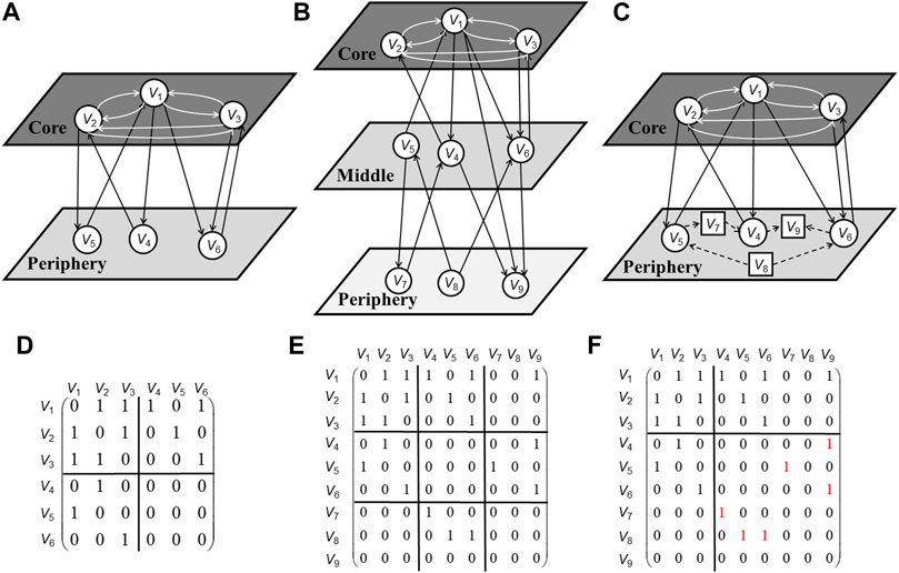
FIGURE 1. Ilustration of the core–periphery and core–middle–periphery models. (A) shows the schematic diagram of the idealized core-periphery structure. (D) shows the adjacency matrix corresponding to (A). (B) gives the schematic diagram of the idealized core–middle–periphery model with three core nodes, three middle, and three periphery nodes. (E) shows the adjacency matrix corresponding to (B). (C) shows a possible result of modelling the market structure in (B) by the core–periphery model without the middle layer. (F) shows the adjacency matrix corresponding to (C) with red “1”s indicating the errors in the periphery layer.

All the aforementioned studies suppose that the two-layer core-periphery analytical framework captures the evolution mechanism of the banking system. Apart from the above studies, there are relatively few studies on the true stratification structure of the China banking system. One reason is the limitation of available underlying microdata. The other reason is the neglect of the real-world complex lending relationships between banks in liquidity distribution, which may contribute to the inaccuracy of depicting the banking network as a typical core-periphery structure. Actually, a special tiering structure existed in China’s financial system and the banking system in China could be naturally divided into at least three layers from the market function perspective and regulatory perspective. The core banks generally are flush with liquidity, whereas the periphery banks tackling with long-term funding gap lack a stable relationship with the core banks. The banks in the middle layer help to finance the periphery banks and improve the liquidity redistribution between the core and the periphery in the network. Inspired by the above ideas, we propose a three-layer network model, namely the core-middle-periphery (CMP) model, to analyze the Chinese banking system.

In this study, we empirically investigate the liability network between banks in China spanning 2008–2019, and the statistical results show that the average path length of the network lies in the interval of [2, 3], suggesting that most of the nodes are more than two steps away from each other, so the two-tier core-periphery structure may not be sufficient to portray the complex market hierarchy. The neighbor connectivity and degree distribution also indicate existence of a large number of medium-degree nodes between large-degree nodes and small-degree nodes in the network. In the CMP model, the nodes belonging to the core layer are connected tightly with each other, and the nodes in the middle layer bridge the funding gap between the nodes in the core and periphery layers. We do not put strict internal structural constrain on the banks in the middle layer and encourage more lending activities from the middle to the periphery.

According to the definition of the CMP model, we present an algorithm to separate China bank nodes into three layers correspondingly. The empirical results show that the CMP model captures the crucial characteristic of the China banking structure. Moreover, compared with the traditional CP model, the CMP model detects a narrower subset of core bank nodes, which is conducive to detecting core bank groups in the China banking system more accurately.

Figure 1A shows the schematic diagram of the idealized core-periphery structure proposed by Craig et al. [17]. Figure 1D shows the adjacency matrix A_C−P corresponding to Figure 1A. The arrow of a link indicates the direction of credit exposure, and we set the presence or absence of a link by 1 or 0. Node V₁, V₂, and V₃ belong to the core subset C, which could connect with each other. Node V₄, V₅, and V₆ belong to the periphery subset P. They do not lend to each other, so the periphery block of A_C−P is a square matrix of 0. The periphery nodes only trade with the core nodes, and each core node borrows from and lends to at least one periphery node. Accordingly, to simplify the algorithm procedure, Craig et al. [17] set the off-diagonal blocks of idealized A_C−P as “row regular” with at least one link in every row and “column regular” with at least one in every column, as indicated in Figure 1D.

Figure 1B gives the schematic diagram of the idealized CMP model with three core nodes, three middle, and three periphery nodes. Figure 1E shows the adjacency matrix A_C−M−P corresponding to Figure 1B, where node V₁, V₂, and V₃ belong to the core layer subset C, which connect with each other, so the core block of A_C−M−P is a square matrix (ignoring the zero diagonal as we exclude self-loops, which indicates that banks could not lend to themselves). Node V₄, V₅, and V₆ belong to the middle layer subset M, and the links between middle nodes are unconstrained; In other words, they may either lend to or not lend to each other. Node V₇, V₈, and V₉ belong to the periphery subset P, which only have connections with nodes in the middle layer and have no connections among themselves. Therefore, the periphery block of A_C−M−P is a square matrix of 0. The remaining blocks depict the links between the core, middle and periphery nodes. Each core node borrows from and lends to at least one node in the middle or periphery layers, whereas each node in the middle layer borrows from and lends to at least one node in the periphery layer; Accordingly the related blocks are “row regular” or “column regular”, as indicated in Figure 1E. Moreover, it is much more preferable if nodes in the middle subset lend out to more nodes in the periphery subset, which may facilitate the financing of the periphery layer.

Figure 1C,F show that compared with modeling by the idealized CMP model, if we model the China banking network by the CP model without the middle layer, node V₁, V₂, and V₃ will still belong to the core bank subset C, whereas node V₄, V₅, V₆, V₇, V₈, and V₉ are all classified into the periphery subset P. In this study, we argue that the CP model is insufficient to portray the complex tiering structure with more than two layers. It should be noted that although in this example errors only arise from the periphery, there are cases that errors arise from both the core and periphery layers.

Statistical properties of empirical data

Network definition

Based on bilateral liability data between China banks, the China banking network is given as following: G_real(V, E) consists of |V| = N nodes and |E| = M unweighted-directed edges, where V = {v₁, v₂, …, v_N} denotes the set of bank nodes and E = {e_ij|i, j ∈ N} illustrates the lending relationships between banks. The topology of the China banking network can also be represented by the adjacency matrix ${\mathbf{A}}_{\mathbf{real}}={\{a_{ij}\}}_{N\times N}$, where a_ij = 1 means a link going from node v_i to node v_j (i.e., bank v_i lends to bank v_j); otherwise, a_ij = 0.

Data description

In this study, we collect bilateral liability data between China banks from 1 January 2008 to 31 December 2019 to construct a bank network. In this study, we construct the lending network for each year, and finally give an ensemble network.

Empirical results

In this study, we start by providing a set of network metrics (for definition and calculation of metrics refer to Barabasi [23]) for the China banking system in order to analyze its statistical regularities and topological properties, which may affect the resilience and risk contagion of the network.

The results of the metrics (Table 1) show that the average clustering coefficient (ACC) of the network is significantly higher than that of a random network of the same dimension, and the average path length (APL) is significantly lower than lnN while close to lnlnN, suggesting that the network may have thick-tailed characteristics and follow small-world properties (Barabasi [23], Manoj et al. [24]), indicating that the bank nodes are able to lend to each other through a small number of steps. The average neighborhood degree ⟨k⟩ expands rapidly as the market developed over years. However, the APL, distance (D), and density (S) stay small, suggesting that the network does not become sparser when it becomes larger.

TABLE 1

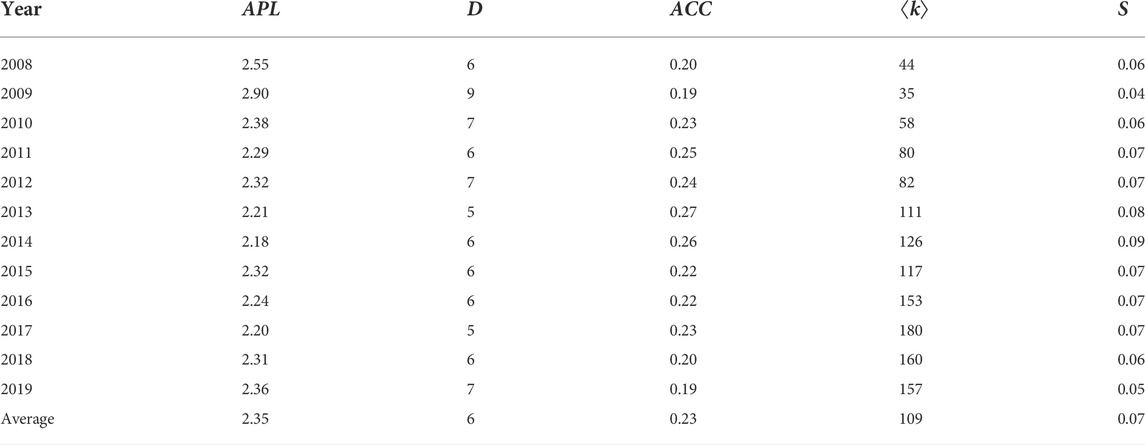
TABLE 1. Network metrics for the China banking system.

From a regulatory perspective, there exists a special tiering structure in China’s financial system. The large-size banks generally are flush with liquidity, whereas small and medium-size banks tackling with long-term funding gaps. However, owing to its high credit risk, asymmetric market information, and disparity of lending volume between large and small-size banks, a portion of small and medium-size banks lack stable lending relationships with large-size banks. Therefore, the banking system in China is naturally divided into three layers: the first layer is consist of the central bank’s open market operation primary dealers and money market makers, which form the core of the banking system; the second layer is consist of qualified financial institutions with sound internal control, which are the main participants of the banking system; the third layer is the small and medium-sized financial institutions that rely on funding relationships with the first two tiers of financial institutions. Therefore, we present the CMP model to regenerate the China banking system with three layers.

Further statistical results show that nodes with large-degree have smaller clustering coefficients and larger betweenness, which indicates that as the intermediary property of large-degree nodes strengthens, the probability of lending among their “neighbors” decreases and thus the “cluster community” is reduced. The APL of the network lies in the interval of (2, 3), indicating that most of the nodes are more than two steps away from each other, suggesting that the two-layer core-periphery structure may not be sufficient to regenerate the hierarchal structure. From the statistical results of the China banking network, the small-degree nodes or node with fewer neighbors tend to connect with nodes with a similar degree, which lead to positive assortativity. On the other hand, when the node degree is large, they tend to trade with small-degree nodes, leading to negative assortativity. Such a phenomenon suggests that bank nodes may contain three subsets with different properties. The degree distribution also shows that, although the network degree distribution has a fat-tailed feature with more small-degree nodes and fewer large-degree nodes, a large number of medium-degree nodes exist in the network, which implies a more complex market hierarchy (Brassil and Nodari [20]).

Inspired by the aforementioned analysis, this study constructs the CMP model containing three subsets of bank nodes and proposes an algorithm to divide the bank nodes into the corresponding three layers. The total error function and the transition probability matrix show that the CMP model and the algorithm could capture the evolution mechanism more accurately.

Model

Traditional idealized core–periphery model

The idealized CP model [17] sets the bank liability relationships as directed networks and defines the ideal CP network G_C−P(V,E) consisting of two subsets of nodes, namely, the core bank layer $\mathbf{C}=\{c_1,c_2,\dots ,c_{N_c}\}$ and the periphery bank layer $\mathbf{P}=\{p_1,p_2,\dots ,p_{N_p}\}$, where $c_{N_c}\in \{\mathrm{2,3}\dots ,N-1\}$, N = N_c + N_p. The idealized CP model’s adjacency matrix is ${\mathbf{\text{A}}}_{\mathbf{\text{C}}\mathbf{-}\mathbf{P}}={\{a_{ij}\}}_{N\times N}$, in which a_ij = 1 denotes node v_i lending to v_j, whereas a_ij = 0 indicates no lending relationship between node v_i and v_j.

For any given N_c, an idealized CP model (see Figure 1A,D) is constructed as follows: Step 1, a number of banks(N_c) in the core layer lend to and borrow from each other; Step 2, the remaining (N − N_c) periphery banks do not lend to or borrow from each other; Step 3, each core bank lends to at least one periphery bank node; Step 4, each core bank borrows from at least one periphery bank node.

The adjacency matrix A_C−P of idealized CP structure can be represented as four blocks, namely, A_CC, A_PC, A_CP, and A_PP (Eq. 1). The core submatrix A_CC is an N_c*N_c matrix of ones with zero diagonals, representing the existence of directed links between all core nodes. Periphery banks do not transact with each other, so the submatrix A_PP is an (N − N_c)*(N − N_c) matrix of zeros. Since the most restricted form of the off-diagonal matrix is a 1-block, which is the upper limit of relationships between core and periphery and too rare to be found in the real-world network, Craig et al. [17] set the threshold of detecting the core-periphery relationship by adopting the off-diagonal blocks in the idealized core–periphery model as row regular and column regular. To be more specific, A_CP (core lending to periphery) block is a row regular (RR) submatrix, suggesting that it contains at least one link in every row. Similarly, since each core bank borrows from at least one periphery bank, the A_PC submatrix is a column regular (CR) matrix with at least one in every column. Figure 1D is an example of the adjacency matrix of the CP model with N = 6 and N_c = 3.

${\mathbf{A}}_{\mathbf{C}-\mathbf{P}}=\left(\begin{array}{cc}\hfill {\mathbf{A}}_{\mathbf{C}\mathbf{C}}\hfill & \hfill {\mathbf{A}}_{\mathbf{C}\mathbf{P}}\hfill \\ \hfill {\mathbf{A}}_{\mathbf{P}\mathbf{C}}\hfill & \hfill {\mathbf{A}}_{\mathbf{P}\mathbf{P}}\hfill \end{array}\right)=\left(\begin{array}{cc}\hfill \mathbf{1}\hfill & \hfill \mathbf{R}\mathbf{R}\hfill \\ \hfill \mathbf{C}\mathbf{R}\hfill & \hfill \mathbf{0}\hfill \end{array}\right).(1)$

The A_C−P is the benchmark for evaluating whether there is a core–periphery structure in the adjacency matrix A_real of the observed network G_real(V, E). As the real-world networks are unlikely to match the ideal theoretical CP structure exactly, the objective of the empirical analysis is to apply an algorithm to find the optimal set of C in A_real, which achieves the best structural match between A_real and A_C−P which both contain N_c core nodes. To be more specific, for any given assignment of banks into C and P subset, the structural inconsistencies between A_real and its nearest tiering model A_C−P could be measured by an error function. The error describes differences in each block between an ideal model and the real-world network. The total error is the result of summing up and standardized errors in all the blocks between an ideal model and the real-world network. The error function is the equation used to obtain the total error.

In order to measure the difference between the empirical network structure A_real and the idealized traditional CP model A_C−P, firstly we define the difference E comprising of four elements, in which the sum of all missing links (outside the diagonal) in the core layer is defined as E_CC, the cumulative value of all observed links among the periphery layer is defined as E_PP, and off-diagonal errors are calculated by E_CP and E_PC, respectively. To be more specific, for the off-diagonal blocks, a zero row in A_CP indicates that a core bank does not lend to any of the (N − N_c) banks in the periphery layer, which is not consistent with the defined feature of core banks, resulting in an error of (N − N_c)*1 in this row, and errors in each row add up to E_CP. Similarly, a zero column in A_PC shows that this core bank does not borrow from any periphery, resulting in an error of (N − N_c)*1 in this column, and errors in each column are summed up to E_PC.

The aggregated errors in each of these blocks are thus given by the following sums:

$\mathbf{E}=\left(\begin{array}{cc}\hfill N_c\times \left(N_c-1\right)-\sum _{i\in \mathbf{C}}\sum _{j\in \mathbf{C}}{a}_{ij}\hfill & \hfill \left(N-N_c\right)\sum _{i\in \mathbf{C}}\mathit{max}\left\{\mathrm{0,1}-\sum _{j\in \mathbf{P}}{a}_{ij}\right\}\hfill \\ \hfill \left(N-N_c\right)\sum _{j\in \mathbf{C}}\mathit{max}\left\{\mathrm{0,1}-\sum _{i\in \mathbf{P}}{a}_{ij}\right\}\hfill & \hfill \sum _{i\in \mathbf{P}}\sum _{j\in \mathbf{P}}{a}_{ij}\hfill \end{array}\right).(2)$

The aggregated error measures the difference between A_real and A_C−P by adding up the E_CC, E_PP, E_CP, and E_PC. As subset C is an internally tightly connected small community, that is, a subset of intermediary bank subset I in which each node has at least one outgoing link and one incoming link. The total error η_C−P of the model is obtained by aggregating and standardizing errors in the following way:

${\eta }_{\mathbf{C}-\mathbf{P}}=\frac{E_{\mathbf{CC}}+E_{\mathbf{PP}}+E_{\mathbf{CP}}+E_{\mathbf{PC}}}{{\sum }_i{\sum }_j{a}_{ij}}=\frac{E_{\mathbf{CC}}+E_{\mathbf{PP}}}{{\sum }_i{\sum }_j{a}_{ij}}.(3)$

Take Figure 2 as an example, the missing link between V₁ and V₂ is an error among core banks(E_CC); the existing link between V₄ and V₆ is an error among periphery banks(E_PP); and the missing links from V₃ to V₄, V₅, and V₆ generate an error(E_CP) in the off-diagonal blocks. The difference between idealized model and real-world network in Figure 2 is calculated as total error which equals to 5 (η_C−P = E_CC + E_CP + E_PP = 1 + (N − N_c)*1 + 1 = 1 + 3*1 + 1 = 5).

FIGURE 2

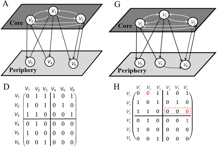
FIGURE 2. (Color online) Example of calculating error score between idealized CP model A_C−P (A,D) and real-word network A_real (G,H).

We could develop algorithms to minimize the η_C−P in order to find the optimal division solution. The optimal solution R* is the result with the optimal set of cores which generates the smallest distance to the idealized CP model of the same dimension. Γ is the set of all possible solution set R:

${\mathbf{\text{R}}}^{\ast }=\mathrm{arg\; min}{\eta }_{\mathbf{C}-\mathbf{P}}\left(\mathbf{R}\right)=\left\{\mathbf{R}\in \mathbf{\Gamma }|\eta \left(\mathbf{R}\right)\le \eta \left(r\right),\forall r\in \mathbf{\Gamma }\right\}.(4)$

Idealized core–middle–periphery model

By introducing the middle layer, this study develops the CMP model. The idealized CMP network G_C−M−P(V,E) consists of core layer subset $\mathbf{C}=\{c_1,c_2,\dots ,c_{N_c}\}$, middle layer subset $\mathbf{M}=\{m_1,m_2,\dots ,m_{N_m}\}$, and periphery layer subset $\mathbf{P}=\{p_1,p_2,\dots ,p_{N_p}\}$, with N_c, N_m, and N_p as number of nodes in C, M and P respectively. The middle banks, which do not have internal transaction constraints and may lend to or not lend to each other freely, are supposed to improve connections between layer C and P, assuming the role of expanding the financing sources of banks in the periphery layer P.

To be more specific, for any given N_c and N_m, an idealized CMP structure G_C−M−P(V,E) is defined as:

(a) All the N_c core banks lend with each other, and all the (N − N_c − N_m) periphery banks do not lend with each other;

(b) Each bank in the core layer lends to (some) non-core banks, and each bank in the core layer borrows from (some) non-core banks;

(c) Each bank in the middle layer lends to (some) periphery banks, and each bank in the middle layer borrows from (some) periphery banks;

(d) Each bank in the middle layer lends to as many banks in the periphery layer as possible.

According to feature (a)–(c), we define the intermediary bank subset I = {i₁, i₂, …, i_z}, in which banks acting both as lenders and borrowers. Intermediary nodes cannot be classified into the subset C if they do not lend to and borrow from non-core nodes. Meanwhile, intermediary nodes that are not classified in the core subset also cannot be classified into the subset M if they do not lend to and borrow from periphery nodes.

1) CMP adjacency matrix A_C−M−P. The adjacency matrix of idealized CMP model is

${\mathbf{A}}_{\mathbf{C}-\mathbf{M}-\mathbf{P}}=\left(\begin{array}{ccc}\hfill {\mathbf{A}}_{\mathbf{C}\mathbf{C}}\hfill & \hfill {\mathbf{A}}_{\mathbf{C}\mathbf{M}}\hfill & \hfill {\mathbf{A}}_{\mathbf{C}\mathbf{P}}\hfill \\ \hfill {\mathbf{A}}_{\mathbf{M}\mathbf{C}}\hfill & \hfill {\mathbf{A}}_{\mathbf{M}\mathbf{M}}\hfill & \hfill {\mathbf{A}}_{\mathbf{M}\mathbf{P}}\hfill \\ \hfill {\mathbf{A}}_{\mathbf{P}\mathbf{C}}\hfill & \hfill {\mathbf{A}}_{\mathbf{P}\mathbf{M}}\hfill & \hfill {\mathbf{A}}_{\mathbf{P}\mathbf{P}}\hfill \end{array}\right)=\left(\begin{array}{ccc}\hfill \mathbf{1}\hfill & \hfill {\mathbf{A}}_{\mathbf{C}\mathbf{M}}\hfill & \hfill {\mathbf{A}}_{\mathbf{C}\mathbf{P}}\hfill \\ \hfill {\mathbf{A}}_{\mathbf{M}\mathbf{C}}\hfill & \hfill {\mathbf{A}}_{\mathbf{M}\mathbf{M}}\hfill & \hfill {\mathbf{A}}_{\mathbf{M}\mathbf{P}}\hfill \\ \hfill {\mathbf{A}}_{\mathbf{P}\mathbf{C}}\hfill & \hfill {\mathbf{A}}_{\mathbf{P}\mathbf{M}}\hfill & \hfill \mathbf{0}\hfill \end{array}\right).(5)$

In the idealized CMP adjacency matrix A_C−M−P, the core bank block A_CC is a 1-block and the periphery bank block A_PP is a 0-block, which are exactly the same as those of the CP adjacency matrix A_C−P.

For the off-diagonal blocks, we also introduce the “row-regular” and “column-regular” patterns. There is at least one inward link and one outward link between each core bank and the non-core banks, presenting as at least one non-zero element in each row of the N_c*(N − N_c) matrix of sub-blocks containing A_CM and A_CP. Similarly, there is at least one inward link and one outward link between each middle bank and the periphery bank layer, that is at least one non-zero element exists in each column of the (N − N_c)*N_c matrix of blocks containing A_MC and A_PC. Accordingly, the submatrix A_MP is row regular and A_PM is column regular. According to the role of the middle bank nodes, there is no internal constraint on the A_MM. The example in Figure 1E shows one idealized CMP adjacency matrix with N = 9, N_c = 3, and N_m = 3. It should be noted that in G_C−M−P(V,E), for any given N_c and N_m, we can depict a series of idealized CMP models with different A_C−M−P, featuring various patterns of off-diagonal blocks which all satisfy the “row regular” and “column regular” pattern.

2) Error function. In order to find the three layers, say C, M and P, from the empirical China banking network, it is natural to minimize the total error between A_real and A_C−M−P of the same dimension as the optimization function.

Moreover, we treat the A_MP differently based on the fact that middle banks’ lending to periphery banks helps to compensate for the missing links between the core and periphery banks, which help to close the funding gap of periphery banks as well as improve redistribution of liquidity in the banking system. As more lending relationships from middle to periphery is desirable but not compulsory in the model, it is not feasible to design the idealized block A_MP as a 1-block, which means that missing links from middle to periphery would be punishment items and contribute to a higher total error. In addition, it is much more complicated to design a variable A_MP in the idealized model with more than one lending relationship from middle to periphery. To solve this problem, we calculate the number of links indicating M’s lending to P as the reward term to emphasize the role of the middle layer in terms of providing liquidity to the periphery layer and to simplify the searching procedure. The more lending links, the smaller the total error is.

Compared with the idealized CMP model, we develop an algorithm to minimize the total error function. Since it is complicated to obtain the optimized C, M and P subsets simultaneously, we design a two-step algorithm to simplify the searching procedure.

Step1: Select the intermediary set I = {i₁, i₂, …, i_z} from all bank set of the G_real network, where Z ∈ {1, 2, …, N};

Step2: Filter out the core set C by using the following method. Given a determined core size N_c, where N_c ∈ {1, 2, …, Z}, searching for the optimal core set C in I using simulated annealing by minimizing the total error. Then the remaining banks are set into the bank set T={t₁,t₂,…,t_N−Nc};

Step3: Filter out the middle set M by using the following method. After fixing each core set result C in Step 2, filter out the middle bank set M from subset T. To be specific, after choosing each middle size N_m, where N_m ∈ {1, 2, …, Z − N_c}, we search for the optimal middle set M ∈ {I\C} to minimize the total error and group the remaining banks into P.

Step4: Based on the total error calculated by the C, M, and P allocation in Step 3, find another candidate core size N_c ∈ {1, 2, …, Z} and repeat Step 2 to search for the optimal core set C. Then repeat Step 3 to search for the optimal middle set M. Stop the iteration when the difference of total error for timestep t − 1 and t is smaller than the threshold and output the final set of C, M and P.

The total error function η_C−M−P is defined as the standardized difference between idealized CMP model A_C−M−P and real-world network A_real. According to the two main steps of the algorithm, the total error is divided into two parts, namely, E₁ and E₂ which are defined as follows.

${\mathbf{E}}_1=\left(\begin{array}{cc}\hfill N_c\times \left(N_c-1\right)-\sum _{i\in \mathbf{C}}\sum _{j\in \mathbf{C}}{a}_{ij}\hfill & \hfill \left(N-N_c\right)\sum _{i\in \mathbf{C}}\mathit{max}\left\{\mathrm{0,1}-\sum _{j\in \mathbf{T}}{a}_{ij}\right\}\hfill \\ \hfill \left(N-N_c\right)\sum _{j\in \mathbf{C}}\mathit{max}\left\{\mathrm{0,1}-\sum _{i\in \mathbf{T}}{a}_{ij}\right\}\hfill & \hfill \sum _{i\in \mathbf{T}}\sum _{j\in \mathbf{T}}{a}_{ij}\hfill \end{array}\right),(6)$

${\mathbf{E}}_2=\left(\begin{array}{cc}\hfill 0\hfill & \hfill p\sum _{i\in \mathbf{M}}\mathit{max}\left\{\mathrm{0,1}-\sum _{j\in \mathbf{P}}{a}_{ij}\right\}\hfill \\ \hfill p\sum _{j\in \mathbf{M}}\mathit{max}\left\{\mathrm{0,1}-\sum _{i\in \mathbf{P}}{a}_{ij}\right\}\hfill & \hfill \sum _{i\in \mathbf{P}}\sum _{j\in \mathbf{P}}{a}_{ij}\hfill \end{array}\right).(7)$

For each determined core size N_c and corresponding potential sets of C in Step 2, we continue to select potential node set M in Step 3. After selecting each potential node set M, we are able to calculate the corresponding E_MM, E_MP, E_PM, and E_PP, where E_PP is defined as the number of connected links between periphery banks, E_MP denotes the number of missed relationships in terms of middle banks subset lending to periphery banks, and E_PM measures the number of missed relationships in terms of middle banks subset borrowing from periphery banks. The middle bank block error E_MM is zero as there is no constrain for node-set M. In order to enhance the importance of M in the error calculation process, we add a reward term $E_{\mathbf{MP}}^{\prime }$ (Eq. 8) into the error function as follows.

$E_{\mathbf{MP}}^{\prime }=-\sum _{i\in M}\sum _{j\in P}{a}_{ij}.(8)$

Then the total error function η_C−M−P is given as follows.

${\eta }_{\mathbf{C}-\mathbf{M}-\mathbf{P}}=\frac{E_{\mathbf{CC}}+E_{\mathbf{CT}}+E_{\mathbf{TC}}+E_{\mathbf{TT}}+E_{\mathbf{MP}}+E_{\mathbf{PM}}+E_{\mathbf{PP}}+E_{\mathbf{MP}}^{\prime }}{{\sum }_i{\sum }_j{a}_{ij}}.(9)$

The optimal bank layer classification result R* can be obtained by minimizing the total error function as follows

$\begin{array}{ll}\hfill {\mathbf{R}}^{\ast }& =\mathrm{arg\; min}{\eta }_{\mathbf{C}-\mathbf{M}-\mathbf{P}}\left(\mathbf{R}\right)\hfill \\ \hfill & =\left\{\mathbf{R}\in \mathbf{\Gamma }|{\eta }_{\mathbf{C}-\mathbf{M}-\mathbf{P}}\left(\mathbf{R}\right)\le {\eta }_{\mathbf{C}-\mathbf{M}-\mathbf{P}}\left(r\right),\forall r\in \mathbf{\Gamma }\right\}.\hfill \end{array}(10)$

The algorithm pseudo‐code is given as follows (Algorithms 1-3). θ_stage represents the threshold of number of intermediary nodes in each step.

Algorithm 1. The heuristic process to get an optimized CMP combination.

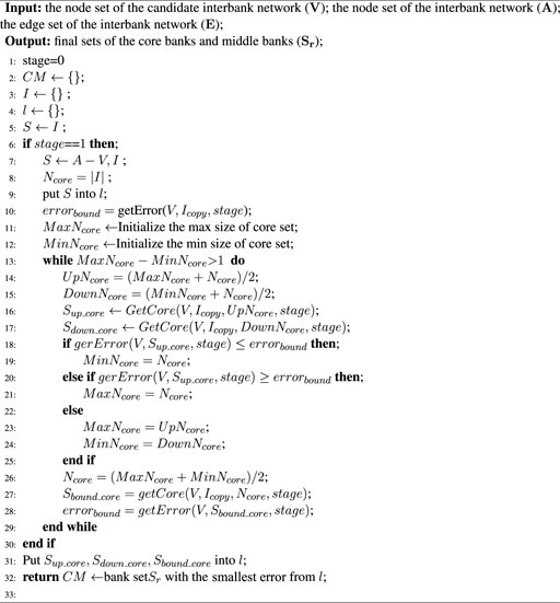
Algorithm 2. The simulated annealing optimizer to get a candidate core with fixed core size.

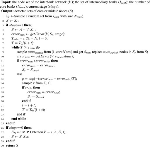
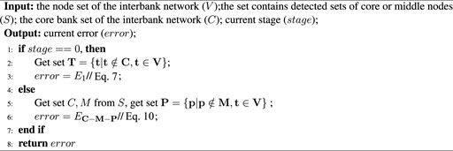
Algorithm 3. Calculation of total error function.

Results

In addition to the total error, this study uses a transition matrix to track the evolution properties of the nodes in different layers. For the bank set sequence X = {X₁, X₂, …, X_t}, where X_t denotes the set of states of each bank at moment t, and its corresponding state space S = {c, m, p, Exit, New} denotes the node status of the core bank, middle bank, periphery bank, exit bank, and new bank, respectively. We defined the transition matrix H(X_t = s|X_t−1 = s′) = Q(s)/Q(s′) as probability of banks moving from state s′ at moment t − 1 to state s at moment t, and Q(s) denotes the number of nodes with state s. The transition matrixes of the CP model and the CMP model are as follows:

${\mathbf{H}}_{\mathbf{C}-\mathbf{P}}\left(\mathrm{s}|{\mathrm{s}}^{\prime }\right)=\left(\begin{array}{ccc}\hfill H\left(c|c^{\prime }\right)\hfill & \hfill H\left(p|c^{\prime }\right)\hfill & \hfill H\left(Exit|c^{\prime }\right)\hfill \\ \hfill H\left(c|p^{\prime }\right)\hfill & \hfill H\left(p|p^{\prime }\right)\hfill & \hfill H\left(Exit|p^{\prime }\right)\hfill \\ \hfill H\left(c|Ne{w}^{\prime }\right)\hfill & \hfill H\left(p|Ne{w}^{\prime }\right)\hfill & \hfill H\left(Exit|Ne{w}^{\prime }\right)\hfill \end{array}\right),(11)$

where ∑_s(s|c′) = ∑_s(s|p′) = ∑_s(s|New′) = 1.

${\mathbf{H}}_{\mathbf{C}-\mathbf{M}-\mathbf{P}}\left(\mathrm{s}|{\mathrm{s}}^{\prime }\right)=\left(\begin{array}{cccc}\hfill H\left(c|c^{\prime }\right)\hfill & \hfill H\left(m|c^{\prime }\right)\hfill & \hfill H\left(p|c^{\prime }\right)\hfill & \hfill H\left(Exit|c^{\prime }\right)\hfill \\ \hfill H\left(c|m^{\prime }\right)\hfill & \hfill H\left(m|m^{\prime }\right)\hfill & \hfill H\left(p|m^{\prime }\right)\hfill & \hfill H\left(Exit|m^{\prime }\right)\hfill \\ \hfill H\left(c|p^{\prime }\right)\hfill & \hfill H\left(m|p^{\prime }\right)\hfill & \hfill H\left(p|p^{\prime }\right)\hfill & \hfill H\left(Exit|p^{\prime }\right)\hfill \\ \hfill H\left(c|Ne{w}^{\prime }\right)\hfill & \hfill H\left(m|Ne{w}^{\prime }\right)\hfill & \hfill H\left(p|Ne{w}^{\prime }\right)\hfill & \hfill H\left(Exit|Ne{w}^{\prime }\right)\hfill \end{array}\right),(12)$

where ∑_s(s|c′) = ∑_s(s|m′) = ∑_s(s|p′) = ∑_s(s|New′) = 1.

We defined diagonal elements H(c|c′), H(m|m′), and H(p|p′) in the transition matrix as stability probability W_c, W_m, and W_p, respectively, measuring the probability of nodes remaining unchanged in the core, middle and periphery layers, respectively, for different timesteps. ${\bar{W}}_c$, ${\bar{W}}_m$, and ${\bar{W}}_p$ are defined as the average stability probability of the core, middle and periphery subsets for the entire 12 years. Other elements in the transition matrix are deemed as transition probability, reflecting the probability of nodes moving to other layers. Low stability probability combined with high transition probability indicates that the bank nodes play different roles in different timesteps, which is not consistent with the China scenario. In reality, for most of the banks, the role that each bank plays is relatively stable in the banking system.

In China banking network, the average stability transition probability shows the following results:

${\overline{\mathbf{\text{H}}}}_{\mathbf{\text{C}}-\mathbf{M}-\mathbf{P}}\left(\mathrm{s}|{\mathrm{s}}^{\prime }\right)=\left(\begin{array}{cccc}\hfill 0.78\hfill & \hfill 0.15\hfill & \hfill 0.07\hfill & \hfill 0.00\hfill \\ \hfill 0.02\hfill & \hfill 0.76\hfill & \hfill 0.18\hfill & \hfill 0.04\hfill \\ \hfill 0.02\hfill & \hfill 0.33\hfill & \hfill 0.60\hfill & \hfill 0.05\hfill \\ \hfill 0.00\hfill & \hfill 0.64\hfill & \hfill 0.36\hfill & \hfill 0.00\hfill \end{array}\right),(13)$

${\overline{\mathbf{\text{H}}}}_{\mathbf{\text{C}}-\mathbf{P}}\left(\mathrm{s}|{\mathrm{s}}^{\prime }\right)=\left(\begin{array}{ccc}\hfill 0.50\hfill & \hfill 0.49\hfill & \hfill 0.01\hfill \\ \hfill 0.31\hfill & \hfill 0.64\hfill & \hfill 0.05\hfill \\ \hfill 0.15\hfill & \hfill 0.85\hfill & \hfill 0.00\hfill \end{array}\right).(14)$

Figure 3A shows the empirical error function results of the China banking system. The average total error function of the CMP model is 7%, much smaller than the 20% which is obtained by the CP model. Furthermore, one may find that the total errors of the CMP model range from 3% to 11%, whereas those of the CP model range from 15% to 31%.

FIGURE 3

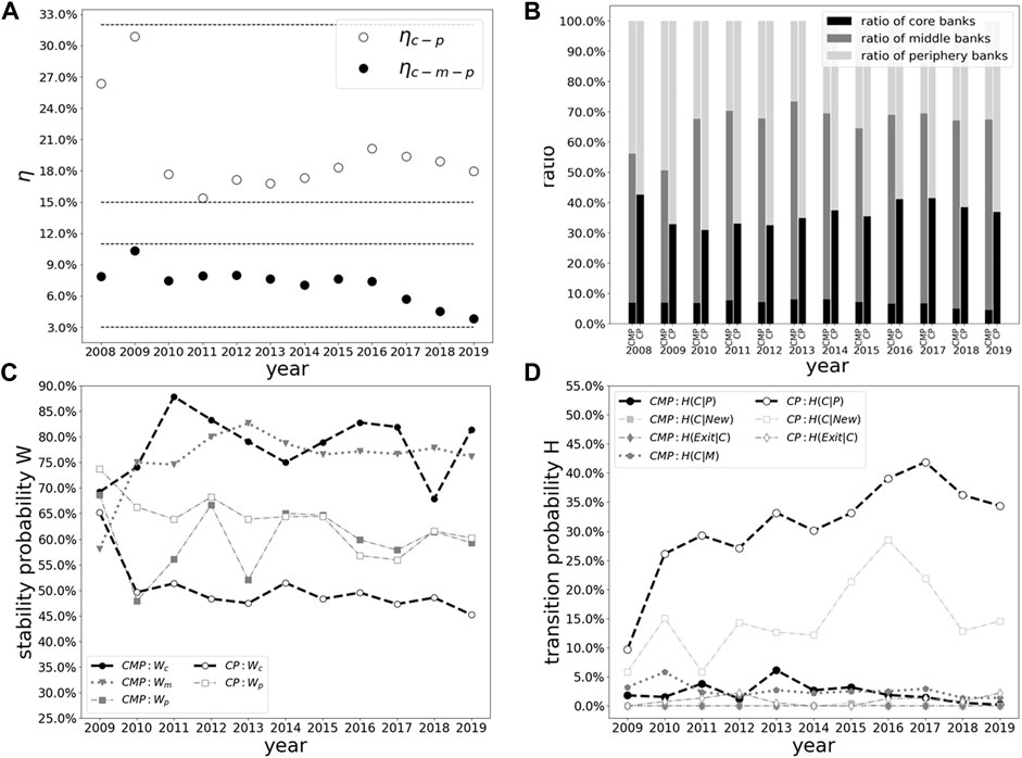
FIGURE 3. (A) Total errors η, (B) ratio of different layers, (C) stability probability W and (D) transition probability H obtained from the China bankinig network by the CMP model and the CP model.

Second, in terms of the number of banks in different layers, the ratios of the core, middle and periphery banks under the CMP model remain stable between 2008 and 2019. Along with the gradual increase of the number of total nodes due to the market development, the numbers of the core, middle, and periphery banks also increase accordingly. Meanwhile, the annual average ratio of core, middle, and periphery banks stays stable (Figure 3B). Specifically, the ratio of core banks stays within the narrow interval of (4%, 9%), suggesting a small and tight core subset over the sample period. In comparison, under the CP model the ratio of core banks fluctuates from 30% to 44% and the ratio of periphery banks fluctuates from 57% to 69% over the sample period, reflecting broader and unstable subsets.

Third, according to the evolution properties of the transition probability, we find that the tiering structure in the CMP model (Figure 3C) is more stable than that of the CP model. Specifically, the composition of the core bank subset remains remarkably stable. Under the CMP model, the annual averages of stability probability ${\bar{W}}_c$, ${\bar{W}}_m$ and ${\bar{W}}_p$ are 78%, 76% and 60%, respectively, indicating a relatively high probability of the core, middle, and periphery banks remaining in the same layer. Specifically, W_c falls within the range of (69%, 88%), which indicates that the categorizing of core banks is relatively stable. In reality, the role of banks in the core layer is very stable, which rarely changes compared with non-core banks. Therefore, compared with the CP model, the CMP model could capture the evolution properties more accurately.

Fourth, as can be seen in Figure 3D, for the CMP model, the average probabilities of a middle and a periphery bank becoming a core bank are as low as 2%. A core bank does not exit the market, and it is difficult for a new entrant to become a core bank in the following year. All these experimental results are reasonable in terms of explaining the real-world banking system structure. In comparison, according to the empirical result of the CP model, a core bank has a 1% probability of exiting the market, whereas a new entrant and a periphery bank have a 15% and 31% probability of becoming a core bank respectively, which is extremely high comparing with the CMP model. Moreover, a core bank obtained by the CP model has a 49% probability of becoming a periphery bank in the next year which is inconsistent with the fact that the banks in the core layer play an important role in the banking system and have stable characteristics.

Generally speaking, the China banking system exhibits an evident and stable three-layer structure, which is consistent with the proposed CMP model.

Conclusion and discussions

In this study, we present the CMP model to analyze the evolution properties of the China banking network, in which banks are nodes and the existence of lending relationships are directed links. We find that this network shows characteristics commonly found in other empirical networks, such as the small-world phenomenon and fat-tailed degree distribution. However, as China banking system possesses a special three-layer structure, we extend the CP model into the CMP model by adding middle nodes to improve the connection between large-degree nodes and small-degree nodes, so as to better describe the real-world network structure.

The total error function and the stable transition probability show that China banking network is prone to approximate a CMP structure with smaller total error scores, tighter core subset, and stronger structural stability over time rather than a CP structure.

During the sample period, the average total error of optimal CMP structure fitting on the annual China banking network comes to less than 10% of network links, decreasing by 64% from the 20% average total error under the CP model, indicating that the CMP model explains the real network better.

For the CMP model, the ratios of the core, middle, and periphery banks under the CMP model remain stable between 2008 and 2019, featuring a tight core set and a large middle set. In comparison, the sizes of core and periphery banks subets under the CP model are volatile, suggesting that a portion of middle modes are likely to be classified into core banks.

Furthermore, an in-depth analysis of banks in each layer shows that the average stability probability of the core bank subset$({\bar{W}}_c)$ increases from 50%(under the CP model) to 78% by adopting the CMP model, contributing to a more accurate categorizing of core node subset with higher intertemporal stability. The average stability probability$({\bar{W}}_m)$ of the middle bank layer in the CMP model also features a high level of 76%, whereas that of the periphery bank set is 60% $({\bar{W}}_p)$.

In terms of the transition probabilities, a core bank does not exit the market, and it is of quite a low probability for a middle bank, a periphery bank, or a new entrant to become a core bank in the following year under the CMP model, which is consistent with the intuitive understanding of real-world banking system scenario. In contrast, in the CP model, a core bank may exit the market although the probability of this scenario is as low as 1%. Meanwhile, a new entrant and a periphery bank have a 15% and 31% probability of becoming a core bank, respectively.

To sum up, compared with the CP model, the CMP model could regenerate the stable core, middle and periphery structure for China banking network.

In future work, the following issues will be examined. This study lacks a solid theoretical foundation of a three-tier structure which aims to answer the following question: Is a three-tier structure superior to a multi-layer structure in arguing for a Chinese banking network? Whether no internal constraint of middle nodes is rationale and sufficient? What is the optimal size of middle banks since a loose constraint on middle nodes and tight constraint on periphery nodes may lead to a large portion of nodes being dropped into the middle community so as to minimize the total error? What is the exact theoretical relationship between middle nodes, core, and periphery nodes? How to measure the effectiveness of middle nodes’ intermediary role in liquidity distribution? Is there a better way besides adding a reward item to encourage more intermediary behavior of the middle nodes? We would go deep into a theoretical discussion of these three-layer structures in the future.

Moreover, as the size of the network increases, the computation complexity would increase greatly, making it difficult to obtain a global optimum. How to develop fast optimization algorithm through theoretical analysis will be the next research topic. Whether the two-step algorithm could be improved and optimized is also an interesting question. From a network evolution perspective, we present the annual transition matrix to depict stability probability and transition probability. A solid and stable multilayer network is a multiple dimension problem as opposed to the transition of core and periphery nodes in a two-layer model, as more layers may generate complex transition scenarios which are more complicated to analyze and monitor. The role of the core, middle, and periphery may affect the network resilience, and it is challenging to discuss the three-layer network resilience on a time-varying basis.

In the future we plan to explore these aforementioned problems further, laying a much solid foundation for the observed three-tier structure.

Data availability statement

The original contributions presented in the study are included in the article/Supplementary Materials; further inquiries can be directed to the corresponding author.

Author contributions

NC and JL designed and performed the research. DT and YO performed the computations, NC, JL, YC, DT, YO, and MJ wrote the manuscript.

Funding

JL is supported by the National Natural Science Foundation of China (Grant Nos. 72171150, 61773248, 92146004, and 71901144).

Conflict of interest

The authors declare that the research was conducted in the absence of any commercial or financial relationships that could be construed as a potential conflict of interest.

Publisher’s note

All claims expressed in this article are solely those of the authors and do not necessarily represent those of their affiliated organizations, or those of the publisher, the editors, and the reviewers. Any product that may be evaluated in this article, or claim that may be made by its manufacturer, is not guaranteed or endorsed by the publisher.

References

1. Allen F, Gale D. Financial contagion[J]. J Polit Economy (2000) 108(1):1–33. doi:10.1086/262109

CrossRef Full Text | Google Scholar

2. Cassar A, Duffy N. Contagion of financial crises under local and global network [M]. Berlin, Germany: Springer US (2002).

Google Scholar

3. Battiston S, Caldarelli G, May RM, Roukny T, Stiglitz JE. The price of complexity in financial networks[J]. Proc Natl Acad Sci U S A (2016) 113(36):10031–6. doi:10.1073/pnas.1521573113

PubMed Abstract | CrossRef Full Text | Google Scholar

4. Hu Z, Shen Z, Cao S, Podobnik B, Yang H, Wang WX, et al. Locating multiple diffusion sources in time varying networks from sparse observations[J]. Sci Rep (2018) 8(2685). doi:10.1038/s41598-018-20033-9

PubMed Abstract | CrossRef Full Text | Google Scholar

5. Fang H, Wang Y, Wu X. The collateral channel of monetary policy: Evidence from China. NBER Working Papers (2020).

Google Scholar

6. Martinez-Jaramillo S, Alexandrova-Kabadjova B, Bravo-Benitez B, Solorzano-Margain JP. An empirical study of the Mexican banking system’s network and its implications for systemic risk[J]. J Econ Dyn Control (2014) 40:242–65. doi:10.1016/j.jedc.2014.01.009

CrossRef Full Text | Google Scholar

7. Angelini P. Liquidity and announcement effects in the euro area[R]. Rome, Italy: Bank of Italy (2002). p. 451.

Google Scholar

8. Furfine C. Interbank exposures: Quantifying the risk of contagion[J]. J Money, Credit Banking (2003) 35(1):111–28. doi:10.1353/mcb.2003.0004

CrossRef Full Text | Google Scholar

9. Iori G, Masi GD, Precup OV, Gabbide G, Caldarelli G. A network analysis of the Italian overnight money market[J]. Econ Dyn Control (2008) 32(1):259–78. doi:10.1016/j.jedc.2007.01.032

CrossRef Full Text | Google Scholar

10. Bech ML, Atalay E. The topology of the federal funds market[J]. Physica A: Stat Mech its Appl (2010) 389(22):5223–46. doi:10.1016/j.physa.2010.05.058

CrossRef Full Text | Google Scholar

11. Boss M, Elsinger H, Summer M, Thurner S. Network topology of the interbank market[J]. Quantitative Finance (2004) 4(6):677–84. doi:10.1080/14697680400020325

CrossRef Full Text | Google Scholar

12. Soramaki K, Bech ML, Arnold J, Glass RJ, Beyeler WE. The topology of interbank payment flows[J]. Physica A: Stat Mech its Appl (2007) 379(1):317–33. doi:10.1016/j.physa.2006.11.093

CrossRef Full Text | Google Scholar

13. Inaoka H, Takayasu H, Shimizu T, Ninomiya T, Taniguchi K. Self-similarity of banking network[J]. Physica A: Stat Mech its Appl (2004) 339(3-4):621–34. doi:10.1016/j.physa.2004.03.011

CrossRef Full Text | Google Scholar

14. Boss M, Elsinger H, Summer M, Thurner S. Network topology of the interbank market[J]. Quantitative Finance (2004) 4(6):677–84. doi:10.1080/14697680400020325

CrossRef Full Text | Google Scholar

15. Edson B, Cont R. The Brazilian interbank network structure and systemic risk[R]. Brasília, Federal, Brazil: Central Bank of Brazil (2010). p. 219.

Google Scholar

16. Borgatti SP, Everett MG. Models of core/periphery structures[J]. Social Networks (2000) 21(4):375–95. doi:10.1016/s0378-8733(99)00019-2

CrossRef Full Text | Google Scholar

17. CraigVon Peter G, von Peter G. Interbank tiering and money center banks[J]. J Financial Intermediation (2014) 23(3):322–47. doi:10.1016/j.jfi.2014.02.003

CrossRef Full Text | Google Scholar

18. Langfield S, Liu Z, Ota T. Mapping the UK interbank system[J]. J Banking Finance (2014) 45:288–303. doi:10.1016/j.jbankfin.2014.03.031

CrossRef Full Text | Google Scholar

19. Fricke D, Lux T. Core–periphery structure in the overnight money market: Evidence from the e-MID trading platform[J]. Comput Econ (2015) 45(3):359–95. doi:10.1007/s10614-014-9427-x

CrossRef Full Text | Google Scholar

20. Brassil A, Nodari G. A density-based estimator of core/periphery network structures: Analysing the Australian interbank market[R]. Australia: RBA Research Discussion Papers (2018).

Google Scholar

21. Yang H, Hu M. Risk contagion of China’s interbank markets based on Core-Periphery network[J]. J Manage Sci China (2017) 20(10):44–56. (in Chinese).

Google Scholar

22. Xing J, Guo Q, Liu J. Interbank network estimation based on local clustering features[J]. J Univ Electron Sci Technol China (2021) 2021(08). (in Chinese).

Google Scholar

23. Barabási AL. Network science[J]. Philosophical Trans R Soc A (2013) 371(1987):2012.

Google Scholar

24. Manoj BS, Abhishek C, Rahul S. Complex networks: A networking and signal processing perspective[M]. Whitby, ON, Canada: Pearson (2018).

Google Scholar