 Zhao-Long Hu
 Yuan-Zhang Deng
 Hao Peng
 Xiang-Bin Zhu
- College of Mathematics and Computer Science, Zhejiang Normal University, Jinhua, China
Power line inspection plays a significant role in the normal operation of power systems. Although there is much research on power line inspection, the question of how to balance the working hours of each worker and minimize the total working hours, which is related to social fairness and maximization of social benefits, is still challenging. Experience-based assignment methods tend to lead to extremely uneven working hours among the working/inspection teams. Therefore, it is of great significance to establish a theoretical framework that minimizes the number of working teams and the total working hours as well as balances the working hours of inspection teams. Based on two real power lines in Jinhua city, we first provide the theoretical range of the minimum number of inspection teams and also present a fast method to obtain the optimal solution. Second, we propose a transfer-swap algorithm to balance working hours. Combined with an intelligent optimization algorithm, we put forward a theoretical framework to balance the working hours and minimize the total working hours. The results based on the two real power lines verify the effectiveness of the proposed framework. Compared with the algorithm without swap, the total working hours obtained by the transfer-swap algorithm are shorter. In addition, there is an interesting finding: for our transfer-swap algorithm, the trivial greedy algorithm has almost the same optimization results as the simulated annealing algorithm, but the greedy algorithm has an extremely short running time.
1 Introduction
With the development of the society and smart grid, the demand for electricity is increasing, and the range of power lines is also getting wider [1]. The safe operation and maintenance of power lines is related to our high quality of life, but subtle disturbances in the power system may cause great harm [2]. For example, on December 23, 2015, Ukraine reported a service outage [3, 4]. As a part of power systems, the power line inspection is a very important step to ensure the normal operation and maintenance of the power system. However, power lines are always exposed to the outside and are vulnerable to earthquakes, floods, storms, building collapses, etc., so it is necessary to regularly inspect power lines [5, 6]. The power line inspection includes tower inspection and wire inspection. The traditional method of overhead power line inspection is to manually walk along the line or by vehicles and use telescopes and infrared thermal imagers to conduct an inspection. The main problems of traditional inspection are as follows: on the one hand, the distance of the inspected power lines is long and the workload is heavy and the efficiency is very slow. In the event of natural disasters such as earthquakes and landslides, the inspection task will not be carried out. On the other hand, inspection in mountainous areas is of high risk, threatening the life safety of workers. Therefore, how to efficiently complete power line inspection is a very important issue. With the development of technology, unmanned aerial vehicles (UAVs) can be used instead of a human in some cases. Compared with traditional inspection, UAVs have the advantages of strong adaptability, high accuracy, and high work efficiency in power line inspection [7–10]. Workers can control UAVs to take photos and then send them to the terminal. From the terminal, we can find out where the problem is and then use robots to repair it. At present, the robot can only do some simple repair work. If it encounters complex problems, it still needs to be carried out manually [11–14]. Usually, UAVs face limited battery life and controllable distance. As we know, the target power lines are usually far away from the office (work unit). Therefore, the inspection task is implemented with the following two steps. The first step is to drive from the office to the drop-off points of the towers. The second step is to take photos by UAVs and repair them with robots or workers once a problem is detected. At present, the work office mainly relies on experience to assign several inspection teams to inspect the corresponding power lines, resulting in extremely uneven working hours among inspection teams. What is worse is some inspection teams work overtime for a long time. Thus, an efficient solution for balancing the working hours of each inspection team can solve this social fairness problem to a certain extent. With regard to the second step of the inspection work, the inspection time for each tower and the corresponding power line can be considered a constant. This assumption is reasonable because we usually do not know in advance whether these towers need to be repaired. Thus, in order to balance the working hours and minimize the total working hours, we only need to provide optimal power line inspection path planning before performing the inspection task.
Given a target power line, the optimal path planning problem can be transformed into a traveling salesman problem (TSP) or vehicle routing problem (VRP). That is, the inspection team starts from the office and finally returns to the original starting location. Here, all the target towers and the corresponding power lines should be inspected and can only be inspected once. Therefore, the problem belongs to the NP-hard problem encountered in combinatorial optimization [15, 16]. The TSP or VRP is a very old and classic problem in graph theory, and many research methods for optimal path planning were proposed [17], such as integer programming [18], dynamic programming [19], and branch and bound algorithm [20, 21]. However, the high computational complexity of those exact algorithms prevents them from being applied to large-scale networks. To improve computational efficiency, agent-based or multi-agent-based heuristic intelligent optimization algorithms were successively proposed. For example, genetic algorithms [22], ant colony algorithms [23], simulated annealing algorithms [24, 25], particle swarm algorithms [26], and some derivative algorithms, or hybrid algorithms [17, 27, 28]. Recently, some optimization methods by machine learning were presented [29], such as graph neural network [30] and reinforcement learning [31].
If there are too many power lines to be inspected, it is not practical to assign one inspection team to complete the inspection task. The problem can be transformed into classical multiple traveling salesman problems (MTSP), which is also NP-hard [32, 33]. The constraint conditions are 1) all the inspection teams should start from the same location (office) and return to the office. 2) Each inspection team must inspect at least one tower. 3) Each tower and the corresponding power line can only be inspected once. Despite this problem seeming difficult, it can still be solved by the abovementioned method [17, 34, 35]. For example, based on k-means clustering, the optimal path planning was carried out in each cluster [36–38]. However, those works did not take into account the balanced workload of each cluster. As workload can reflect social fairness, and the MTSP associated with balancing workload has attracted increasing attention [39–41]. For example, Alves et al. minimized the distance and balanced the routes for the MTSP by genetic algorithms [39]. Xu et al. proposed a two-phase heuristic algorithm to balance the number of destinations of travel agents [40]. Compared with balancing the routes or the number of traveling destinations, it is fairer to balance the working hours. Lee et al. studied the balance of the traveling time for MTSP, but the traveling time among each pair of destinations is linear with the distance [42]. Recently, Vandermeulen et al. investigated the balanced working hours for MTSP by translating the task assignment problem into the minimum Hamiltonian partition problem; however, the traveling/cost time was obtained by simulation [43]. Hu et al. proposed a transfer method to balance the working time with the minimum number of inspection teams with two real power lines [6]. But, there is no need to consider the walking time because the task of taking photos can be implemented by the UAVs.
In this article, considering both driving time and inspection time, we give the theoretical solution for the minimum number of inspection teams. In addition, we propose a transfer-swap algorithm to balance the working hours among inspection teams and minimize to total working hours. Combined with the minimum number of inspection teams and intelligent optimization algorithms, a framework for optimal path planning is presented. Concretely, based on the latitude and longitude of the power grid (line-5876 and line-5803) in Jinhua City and the latitude and longitude of the drop-off points of towers of the two power lines, we obtain both the driving time from the office to all the towers and the driving time among each pair of towers through the web crawler [6]. Compared with the real driving time from the office to each tower, it is found that the driving time obtained by the crawler is not much different from that of the real one. Using the crawled driving time, we can construct a fully connected network of driving time between the office and all towers. Simulations verify the provided theoretical solution for the minimum number of inspection teams, and results from four optimization algorithms prove that the proposed transfer-swap algorithm can well-balance the working hours.
The article is organized as follows. In Section 2, first, we describe our model. Second, we present the theoretical analysis for the minimum number of inspection teams. Third, we provide the transfer-swap algorithm to balance the working hours among inspection teams, which is the key to the general framework for optimal path planning. In Section 3, we analyze two real power lines and verify the framework of optimal path planning with the minimum inspection teams and balancing the working hours. Finally, we conclude and discuss this article in Section 4.
2 Model and Methods
2.1 Optimal Inspection Path Planning Model
Because the location of the office is fixed, we can construct a fully connected network once the target towers are identified. The fully connected network can be described by G = (V, E, T). Here, V is the node-set V = {v0, v1, …, vN}. v0 represents the office and the others are the number of the N target towers, see Figure 1. The edge set
td, the driving time for one single inspection team to visit all the target towers and return to the office.
tins, the inspection time for inspecting each tower and the corresponding power line, which can be completed by UAVs, robots, or workers. The term can be set to a constant, say 15 min. Thus, the total working hours (i.e., spending time) for one single inspection team to complete the task is td + tinsN.
tmax, the maximum working hours on workday for every inspection team. Generally, let us define tmax = 8 h or 28,800 s.
tdiff, the maximum difference of the working hours among inspection teams, quantified by
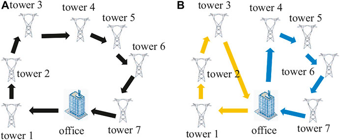
FIGURE 1. (color online) A simple example about path planning with one office and seven towers. (A) Optimal path for one inspection team to complete a given inspection task. The total working hours (spending time) is the driving time of the path plus the inspection time by UAVs, robots, or workers, that is, td + 7tins. (B) Optimal path that balances the working hours between the two inspection teams. The working hours is
The objective is to balance the working hours of each inspection team and minimize the total working hours, see Figure 1. The system model can be written by
Subject to
where
Here, vi, vj ∈ V and
Constraints 2) and 3) ensure all the k inspection teams starting from the office and returning to the office. Constraint sets 4) and 5) are the assignment constraints to make sure that each tower should be preceded by and precedes exactly one another tower. Constraint sets 6) and 7) are the Miller–Tucker–Zemlin sub-tour elimination constraints [18]. Constraints 8) and 9) are weak and are also our optimization objectives.
In this article, we introduce three artificial intelligence algorithms to optimize the inspection path for a given k, tmax,, and ϵ. The three algorithms are the ant colony algorithm (antcol), simulated annealing algorithm (SA), and one hybrid algorithm made up of the genetic algorithm and extremal optimization (GA-EO). The genetic algorithm (GA) has poor local search ability, large computation, poor adaptability to large search space, and easy convergence to a local minimum. The GA-EO algorithm is adopted by combining the EO algorithm with the traditional genetic algorithm [44].
In order to compare with the abovementioned three optimal algorithms, we also present a greedy algorithm. The greedy algorithm is described as follows: For each step, with probability 1 − p, the tower with the shortest driving time is selected as the next inspection target. Otherwise, one unselected tower is randomly selected as the next inspection target with the probability p. If p = 0, it is equivalent to the pure greedy algorithm, so p can be seen as a perturbation parameter. Concretely, it is assumed that the currently visited tower is vi and the tower set containing all the towers that has been visited is defined as Vc. The next tower vj that will be selected to visit with a probability 1 − p should satisfy the condition
2.2 Theoretical Analysis of Minimum Number of Inspection Teams
The minimum number of inspection teams is denoted as the capacitated vehicle routing problem (CVRP) [45]. Several general algorithms were proposed for a minimum number of vehicles, such as greedy algorithm [46], and integer programming [47]. Here, we show a theoretical solution to the minimum number of inspection teams. For one single inspection team to inspect the power line, the working hours are td + Ntins. Here, td is the total driving time on the path and tins is the inspection time to inspect one tower and the power line between the tower and the next tower, which can be set to a constant, such as 15 min. If td + Ntins > tmax, more than one inspection team is required. The required number of inspection teams k satisfies
The equal sign holds if k is equal to 1. If (td + Ntins) > tmax, then k > 1.
Because
From the previousequation, the minimum number of inspection teams satisfies
To find the exact minimum number of inspection teams as quickly as possible, here, we present one alternative approach to estimate the value of k by using the average driving time from the office to all the towers. Specifically, the round-trip time of k inspection teams can be approximately computed by the average round-trip time from the office to all towers, which can be expressed as
Thus, the total working hours for all teams is td + N × tins + (k − 1) × tave. Because there is one round-trip time in td, so we use (k − 1) × tave instead of k × tave. Therefore, the minimum number of inspection teams should satisfy
Here, k is the smallest integer and is not less than
where ⌈⋅⌉ represents the smallest integer not less than ⋅.
In conclusion, the minimum k can be obtained by Eqn. 13; however, we can use Eqs. 11, 16 to estimate it. Without loss of generality, in this article, we assume that the maximum working hours tmax = 8 h of each inspection team on a workday and the tins = 15 min.
2.3 One Framework For Optimal Inspection Path With Balancing Working Hours By the Transfer-Swap Algorithm
Based on the minimum number of inspection teams k in the last section, we propose a new algorithm to balance the working hours and minimum the total working hours by the transfer-swap algorithm and provide the framework for optimal inspection path with several intelligent optimization algorithms.
To be a concert, we first randomly select k towers as center nodes and obtain the k set by K-means based on the driving time matrix T. For example, let us set node vi to be one center node. For non-central node vj ∈ V, add vj to the set of vi if the driving time from vj to vi is minimum among all the center nodes.
Second, based on the optimization algorithms, we can get the optimal path and compute the working hours for each set
Third, if
Fourth, if the condition in the third step is not satisfied, we transfer one tower in the tower set with
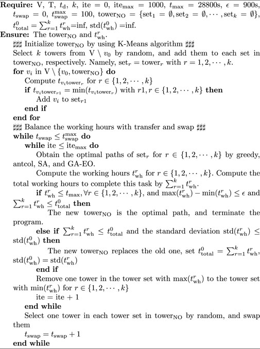
Algorithm 1. Optimal inspection path planning with the transfer-swap algorithm.
3 Results
3.1 The Analysis of Two Real Power Lines
In this section, we analyze the driving time of two real power lines, line-5876 and line-5803, in Jinhua City, Zhejiang Province.
The real data contain the following details [4]:
i) Longitudes and latitudes of all towers for the two power lines and the office. As shown in Figures 2A,B.
ii) Longitudes and latitudes of drop-off points of each tower.
iii) The driving times
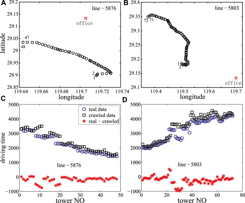
FIGURE 2. (color online) (A,B) Longitudes and latitudes of towers for line-5876 and line-5803. Only the first two towers and the last two towers, as well as the location of the office, are marked. (C,D) Real driving time and the crawled driving time from the office to each tower for line-5876 and line-5803, and the red star curve stands for the difference. There are 48 towers in line-5876 and 72 towers in line-5803.
For our question, the optimal path should start from the office, after inspecting all the target towers and power lines and finally returns to the office. Although data contain the driving time from the office to the drop-off point of each tower, it does not contain the driving time
3.2 Optimize Inspection Path With One Single Inspection Team
In this section, we test our framework with two real power lines. The configuration of our computer is Intel Core (TM) i7-7700 CPU, 16 GB RAM, and 3.6 GHz processing speed. First, we study the inspection path planning for one single inspection team by antcol, SA, GA-EO, and the greedy algorithm. Because the inspection time of each tower and its corresponding power line, tins is considered to be 900s, and it is only necessary to optimize the driving time when assigning a single inspection team. As can be seen from Figures 3A,C, when all targets are inspected, the SA algorithm takes the shortest driving time, followed by the GA-EO algorithm. The greedy algorithm in line 5876 has the longest driving time, while the total driving time of antcol and the greedy algorithm in line 5803 is nearly the same. Figures 3B,D shows the inspection sequence of the two power lines under the four algorithms.
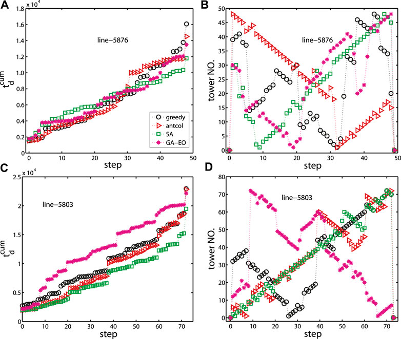
FIGURE 3. (color online) Under the four algorithms (greedy, antcol, SA, and GA-EO); (A,C) the cumulative driving time for a single inspection team to complete the task; (B,D) the optimal inspection path. 0 in tower NO. represents the office, and tower NO means the tower number is to be inspected at that step. (A,B) line-5876. (C,D) Line-5803. The perturbation parameter p = 0.05 for the greedy algorithm.
The result in Figure 3 is from a single simulation. In order to reduce the randomness of the four algorithms, we analyze the results from running independently on 20 times, see Figures 4A,B. It can be seen that the optimal driving time calculated by the SA algorithm is the most stable, and the other three algorithms have a large fluctuation, among which the fluctuation of the greedy algorithm is the largest. In addition, we also find that the driving time by using the SA algorithm is always the shortest, which suggests that SA performs the best path planning. Considering the perturbation parameter p in our greedy algorithm, we further study the driving time with different p for the greedy algorithm in Figures 4C,D. When p = 0, the probability of jumping out of the local optimal value is 0, so the driving time is a constant. When p = 0.1, the result is slightly worse than of p = 0.05. As we can give the optimal path before executing the task, we can simulate it several independent times to find out the inspection path associated with the shortest driving time.
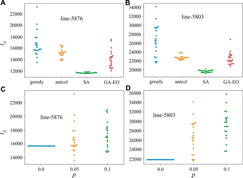
FIGURE 4. (color online) (A,B) Under the four algorithms (greedy, antcol, SA, and GA-EO), the optimal driving time for a single inspection team to perform the inspection task with 20 times of independent running. (C,D) For different perturbation parameters p of the greedy algorithm, the optimal driving time for a single inspection team to perform the inspection task with 20 times running independently. (A,C) Line-5876. (B,D) Line-5803.
In general, the working hours for everyone is not more than 8 h on a workday, namely, tmax = 28800s. Let us assume that the inspection time for each tower is 15 min, that is, tins = 900s. From Figure 3 and Figure 4, we can find that when assigning one single inspection team to perform the inspection task, the working hours of the four algorithms for line-5876 are about 59914s, 58403s, 54918s, and 57409s. For line-5803, the corresponding working hours are about 91433s, 87623s, 84507s, and 87396s. All the working hours exceed the maximum working hours tmax; therefore, more inspection teams are needed. For line-5876, there are 48 towers and the average driving time from the office to each tower is 2221s. For line-5803, there are 72 towers, and the average driving time from the office to each tower is 3252s. From Eqn. 16, the minimum number of inspection teams is one of the elements in the set {2, 3, 4} for line-5876, and the minimum number of inspection teams is one of the elements in {3, 4, 5} for line-5803.
3.3 Optimize Path With the Minimum Number of Inspection Teams
In this section, we analyze and verify the theory of a minimum number of inspection teams and further study and verify our framework for the optimal path planning with the two power lines.
First, we study the optimal path planning with our framework without the swap strategy. From Figure 5, it can be found that when k = 2 and k = 4 for line-5876 and line-5803, respectively, the working hours are not well-balanced, and the working hours of some inspection teams exceed the given tmax = 28800s. For line-5876 with k = 3 and line-5803 with k = 5, the working hours of all inspection teams are within 28800s, and at the same time, the working hours are well-balanced, which is coincided with the theoretical results. Furthermore, we can find that the optimal inspection path of SA has the shortest working hours, while the results of the other three algorithms are almost the same.
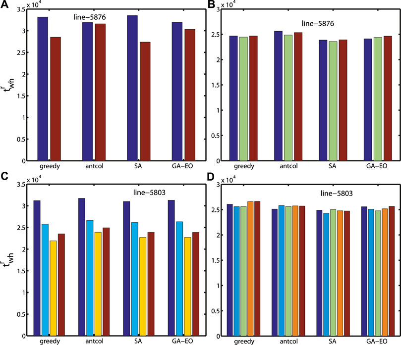
FIGURE 5. (color online) Working hours twh for different numbers of inspection teams by using our framework without swap. (A,B) Line-5876 with k = 2 and k = 3 and (C,D) line-5803 with k = 4, k = 5. The perturbation parameter p is set to 0.05 for the greedy algorithm. Because the working hours are not well-balanced for line-5803 when k = 4, so the result of k = 3 for line-5803 is not shown in this figure.
To compare with the method without a swap strategy, here we embed the swap strategy to optimize the inspection path. From Figures 5B,D) and Figure 6, we can find that the working hours are shorter when combining the transfer and swap strategy for line-5876 and line-5803, which verifies the validity of our proposed transfer-swap algorithm for balancing working hours and minimizing the total working hours. A very interesting result is that with the transfer-swap algorithm, the working hours for the greedy algorithm and SA are very close and work the best, while the working hours for antcol are relatively long. The optimal inspection paths of the k inspection teams with our framework for line-5876 and line-5803 are shown in Figure 7 and Figure 8.
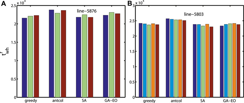
FIGURE 6. (color online) Working hours twh for the minimum number of inspection teams with our framework and transfer-swap algorithm. (A) k = 3 for line-5876 and (B) k = 5 for line-5803. p = 0.05 for the greedy algorithm.
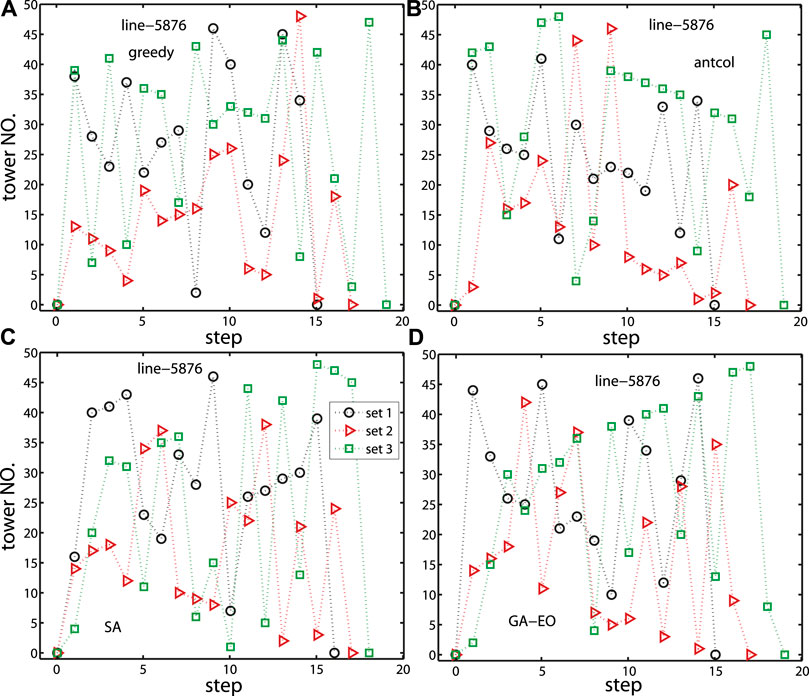
FIGURE 7. (color online) Optimal inspection paths with our framework with (A) greedy, (B) antcol, (C) SA and (D) GA-EO. k = 3 for line-5876. p = 0.05 for the greedy algorithm. Here, the coordinate (0, 0) is the starting point, namely, the office.
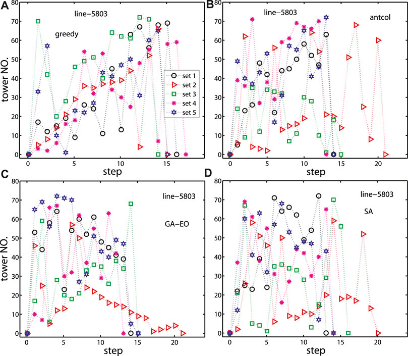
FIGURE 8. (color online) Optimal inspection paths with our framework with (A) greedy, (B) antcol, (C) SA and (D) GA-EO. k = 5 for line-5803. p = 0.05 for the greedy algorithm. Here, the coordinate (0, 0) is the starting point, namely, the office.
Furthermore, we analyze the number of iterations and time-consuming converging to the optimal solution to quantify the performance of our framework under the four algorithms, see Figure 9. It can be found that for line-5876, the number of iterations to converge to the optimal solution is about 15 times. For line-5803, the number of iterations is about 25 times. Figures 9C,D show that the greedy algorithm is very fast and only takes a few seconds, but SA is the slowest and requires about 200s for line-5876 and 500s for line-5803. Therefore, combined with the time-consuming and the working hours, the greedy algorithm performs better than SA, which is a counter-intuitive result. The reason may be that the swap strategy and the perturbation parameter are helpful in avoiding locally optimal solutions.
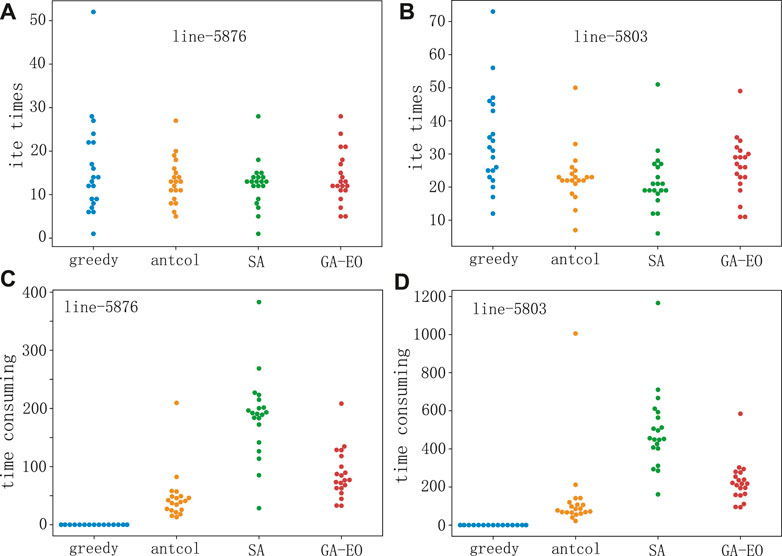
FIGURE 9. (color online) (A,B) Number of iterations converging to the optimal solution with our framework under the four algorithms. The results are obtained by 20 independent simulations. (C,D) Time-consuming (seconds) of converging to the optimal solution with our framework under the four algorithms.
4 Conclusion and Discussion
Taking both driving time and inspection time into consideration, in this study, we study the optimal path planning with the balanced working hours of each inspection team. In order to study the working hours, we have analyzed two real power lines in Jinhua city. In addition, we have provided a range of theoretical solutions for the minimum number of working teams and further have presented a fast method to estimate the theoretical solution, which is the first contribution. In addition, we have proposed a path optimization framework for balancing working hours and minimizing the total working hours based on the minimum number of inspection teams. The key to the proposed framework lies in the transfer-swap algorithm, and it is the second contribution. The simulation results showed that the minimum number of working teams was consistent with our theoretical solution and also verified our framework could balance the working hours and minimize the total working hours. Compared with the optimal results without a swap strategy, the total working hours are shorter when using our proposed transfer-swap algorithm. An interesting finding is that the simulated annealing algorithm (SA) had the shortest total working hours among the four algorithms when the swap strategy is absent. However, when using the transfer-swap algorithm, the working hours obtained by the greedy algorithm were close to those obtained by SA, but the greedy algorithm has the shortest computation time. Thus, with integrated optimization results and running time, it is more efficient to use the greedy algorithm.
In this article, we studied the perturbation parameter p = 0.05 for the greedy algorithm with our framework and did not analyze the pure greedy algorithm with p = 0. This is because the optimization result remains the same for p = 0, so it is easy to fall into a locally optimal solution. In our work, we assumed that the inspection time of each tower was the same. Therefore, there may be some fluctuations in the optimal results when using our framework. A better way to deal with this question is to predict the inspection time of each tower based on historical data. In addition, in our framework, we can use some other optimal algorithms to replace the four methods (greedy, SA, antcol, and EO-GA), such as reinforcement learning or deep learning algorithms.
Data Availability Statement
The original contributions presented in the study are included in the article/Supplementary Material; further inquiries can be directed to the corresponding author.
Author Contributions
Z-LH designed and wrote this manuscript. Y-ZD made the numerical simulations. HP analyzed the results, and all authors discussed and wrote the manuscript.
Funding
This work is supported by the National Natural Science Foundation of China (Nos. 62103375, 62072412, and 62171413), Key Project of Philosophy and Social Science of Zhejiang Province (22NDJC009Z), Social Development Project of Zhejiang Provincial Public Technology Research (Nos. LQ19F030010), MOE (Ministry of Education in China) Project of Humanities and Social Sciences (No. 19YJCZH056).
Conflict of Interest
The authors declare that the research was conducted in the absence of any commercial or financial relationships that could be construed as a potential conflict of interest.
Publisher’s Note
All claims expressed in this article are solely those of the authors and do not necessarily represent those of their affiliated organizations, or those of the publisher, the editors, and the reviewers. Any product that may be evaluated in this article, or claim that may be made by its manufacturer, is not guaranteed or endorsed by the publisher.
References
1. Paul G, Rowena G, Ioana M, Miguel M. Does Electricity Drive Structural Transformation? Evidence from the united states. Labour Econ (2021) 68:101944. doi:10.3386/w26477
2. Sergey VB, Roni P. Catastrophic cascade of Failures in Interdependent Networks. Nature (2010) 464:1025–8.
3. Sullivan JE, Kamensky D. How Cyber-Attacks in ukraine Show the Vulnerability of the u.S. Power Grid. Electricity J (2017) 30(3):30–5. doi:10.1016/j.tej.2017.02.006
4. Hu ZL, Wang L, Tang CB. Locating the Source Node of Diffusion Process in Cyber-Physical Networks via Minimum Observers. Chaos (2019) 29(6):063117. doi:10.1063/1.5092772
5. Van NN, Robert J, Davide R. Automatic Autonomous Vision-Based Power Line Inspection: A Review of Current Status and the Potential Role of Deep Learning. Int J Electr Power Energ Syst (2018) 99:107–20.
6. Hu Z-L, Li J-H, Chen A, Xu F, Jia R, Lin F-L, et al. Optimize Grouping and Path of Pylon Inspection in Power System. IEEE Access (2020) 8:108885–95. doi:10.1109/access.2020.3001435
7. Li Z, Liu Y, Hayward R, Zhang J, Cai J. Knowledge-based Power Line Detection for Uav Surveillance and Inspection Systems. In: 2008 23rd International Conference Image and Vision Computing New Zealand. Christchurch, New Zealand: IEEE (2008). p. 1–6. doi:10.1109/ivcnz.2008.4762118
8. Wang Z, Gao Q, Xu J, Li D. A Review of Uav Power Line Inspection. In: L Yan, H Duan, and X Yu, editors. Advances in Guidance, Navigation and Control. Singapore: Springer (2022). p. 3147–59. doi:10.1007/978-981-15-8155-7_263
9. Pan J-S, Lv J-X, Yan L-J, Weng S-W, Chu S-C, Xue J-K. Golden eagle Optimizer with Double Learning Strategies for 3d Path Planning of Uav in Power Inspection. Mathematics Comput Simulation (2022) 193:509–32. doi:10.1016/j.matcom.2021.10.032
10. Guan H, Sun X, Su Y, Hu T, Wang H, Wang H, et al. Uav-lidar Aids Automatic Intelligent Powerline Inspection. Int J Electr Power Energ Syst (2021) 130:106987. doi:10.1016/j.ijepes.2021.106987
11. Pouliot N, Richard P-L, Montambault S. Linescout Technology Opens the Way to Robotic Inspection and Maintenance of High-Voltage Power Lines. IEEE Power Energ Technol. Syst. J. (2015) 2(1):1–11. doi:10.1109/jpets.2015.2395388
12. Katrasnik J, Pernus F, Likar B. A Survey of mobile Robots for Distribution Power Line Inspection. IEEE Trans Power Deliv (2010) 25(1):485–93. doi:10.1109/tpwrd.2009.2035427
13. Silano G, Bednar J, Nascimento T, Capitan J, Saska M, Ollero A. A Multi-Layer Software Architecture for Aerial Cognitive Multi-Robot Systems in Power Line Inspection Tasks. In: 2021 International Conference on Unmanned Aircraft Systems (ICUAS). Athens, Greece: IEEE (2021). p. 1624–9. doi:10.1109/icuas51884.2021.9476813
14. Carlos HFd.S, Mohamed HA, Daniel M, Campos BAA. Geometrical Motion Planning for cable-climbing Robots Applied to Distribution Power Lines Inspection. Int J Syst Sci (2021) 52(8):1646–63.
15. Croes GA. A Method for Solving Traveling-Salesman Problems. Operations Res (1958) 6(6):791–812. doi:10.1287/opre.6.6.791
16. Dantzig GB, Ramser JH. The Truck Dispatching Problem. Manag Sci (1959) 6(1):80–91. doi:10.1287/mnsc.6.1.80
17. Jiang C, Wan Z, Peng Z. A New Efficient Hybrid Algorithm for Large Scale Multiple Traveling Salesman Problems. Expert Syst Appl (2020) 139:112867. doi:10.1016/j.eswa.2019.112867
18. Miller CE, Tucker AW, Zemlin RA. Integer Programming Formulation of Traveling Salesman Problems. J Acm (1960) 7(4):326–9. doi:10.1145/321043.321046
19. Bellman R. Dynamic Programming Treatment of the Travelling Salesman Problem. J Acm (1962) 9(1):61–3. doi:10.1145/321105.321111
20. Volgenant T, Jonker R. A branch and Bound Algorithm for the Symmetric Traveling Salesman Problem Based on the 1-tree Relaxation. Eur J Oper Res (1982) 9(1):83–9. doi:10.1016/0377-2217(82)90015-7
21. Dell’Amico M, Montemanni R, Novellani S. Algorithms Based on branch and Bound for the Flying Sidekick Traveling Salesman Problem. Omega (2021) 104:102493.
22. Maity S, Roy A, Maiti M. An Imprecise Multi-Objective Genetic Algorithm for Uncertain Constrained Multi-Objective Solid Travelling Salesman Problem. Expert Syst Appl (2016) 46:196–223. doi:10.1016/j.eswa.2015.10.019
23. Escario JB, Jimenez JF, Giron-Sierra JM. Ant colony Extended: Experiments on the Travelling Salesman Problem. Expert Syst Appl (2015) 42(1):390–410. doi:10.1016/j.eswa.2014.07.054
24. Ezugwu AE-S, Adewumi AO, Frîncu ME. Simulated Annealing Based Symbiotic Organisms Search Optimization Algorithm for Traveling Salesman Problem. Expert Syst Appl (2017) 77:189–210. doi:10.1016/j.eswa.2017.01.053
25. Zhou Y, Xu W, Fu Z-H, Zhou M. Multi-neighborhood Simulated Annealing-Based Iterated Local Search for Colored Traveling Salesman Problems. In: IEEE Trans. Intell. Transport. Syst. IEEE (2022). p. 1–11. doi:10.1109/tits.2022.3147924
26. Wang K-P, Huang L, Zhou C-G, Pang W. Particle Swarm Optimization for Traveling Salesman Problem. Proc 2003 Int Conf Machine Learn Cybernetics (2003) 3:1583–5.
27. Baraglia R, Hidalgo JI, Perego R. A Hybrid Heuristic for the Traveling Salesman Problem. IEEE Trans Evol Computat (2001) 5(6):613–22. doi:10.1109/4235.974843
28. Osaba E, Villar-Rodriguez E, Oregi I, Moreno-Fernandez-de-Leceta A. Hybrid Quantum Computing - Tabu Search Algorithm for Partitioning Problems: Preliminary Study on the Traveling Salesman Problem. In: 2021 IEEE Congress on Evolutionary Computation (CEC). Kraków, Poland: IEEE (2021). p. 351–8. doi:10.1109/cec45853.2021.9504923
29. Mele UJ, Gambardella LM, Montemanni R. A New Constructive Heuristic Driven by Machine Learning for the Traveling Salesman Problem. Algorithms (2021) 14(9):267. doi:10.3390/a14090267
30. Yujiao H, Zhen Z, Yuan Y, Xingpeng H, Xingshe Z, Wee SL. A Bidirectional Graph Neural Network for Traveling Salesman Problems on Arbitrary Symmetric Graphs. Eng Appl Artif Intelligence (2021) 97:104061.
31. Zhang Z, Liu H, Zhou M, Wang J. Solving Dynamic Traveling Salesman Problems with Deep Reinforcement Learning. In: IEEE Trans. Neural Netw. Learning Syst. IEEE (2021). p. 1–14. doi:10.1109/tnnls.2021.3105905
32. Tolga B. The Multiple Traveling Salesman Problem: An Overview of Formulations and Solution Procedures. Omega (2006) 34(3):209–19.
33. Jain S. Solving the Traveling Salesman Problem on the D-Wave Quantum Computer. Front Phys (2021) 9:760783. doi:10.3389/fphy.2021.760783
34. Changdar C, Pal RK, Mahapatra GS. A Genetic Ant colony Optimization Based Algorithm for Solid Multiple Travelling Salesmen Problem in Fuzzy Rough Environment. Soft Comput (2017) 21:4661–75. doi:10.1007/s00500-016-2075-4
35. Yan Z, Xiaoxia H, Yingchao D, Jun X, Gang X, Xinying X. A Novel State Transition Simulated Annealing Algorithm for the Multiple Traveling Salesmen Problem. The J Supercomputing (2021) 77:11827–52.
36. Chandran N, Narendran TT, Ganesh K. A Clustering Approach to Solve the Multiple Travelling Salesmen Problem. Int J Ind Syst Eng (2006) 1(3):372–87. doi:10.1504/ijise.2006.009794
37. Yang C, Szeto KY. Solving the Traveling Salesman Problem with a Multi-Agent System. In: 2019 IEEE Congress on Evolutionary Computation (CEC). Wellington, New Zealand: IEEE (2019). p. 158–65. doi:10.1109/cec.2019.8789895
38. Nallusamy R, Duraiswamy K, Dhanalaksmi R, Parthiban P. Optimization of Non-linear Multiple Traveling Salesman Problem Using K-Means Clustering, Shrink Wrap Algorithm and Meta-Heuristics. Int J Nonlinear Sci (2010) 9(2):171–7.
39. Alves RMF, Lopes CR. Using Genetic Algorithms to Minimize the Distance and Balance the Routes for the Multiple Traveling Salesman Problem. In: 2015 IEEE Congress on Evolutionary Computation (CEC). Sendai, Japan: IEEE (2015). p. 3171–8. doi:10.1109/cec.2015.7257285
40. Xiaolong X, Hao Y, Mark L, Marcello T. Two Phase Heuristic Algorithm for the Multiple-Travelling Salesman Problem. Soft Comput (2018) 22:6567–81.
41. Yongzhen W, Yan C, Yan L. Memetic Algorithm Based on Sequential Variable Neighborhood Descent for the Minmax Multiple Traveling Salesman Problem. Comput Ind Eng (2017) 106:105–22.
42. Lee TR, Ueng JH. A Study of Vehicle Routing Problems with Load‐balancing. Int Jnl Phys Dist Log Manage (1999) 29(10):646–57. doi:10.1108/09600039910300019
43. Vandermeulen I, Gross R, Kolling A. Balanced Task Allocation by Partitioning the MultipleTraveling Salesperson Problem. In: 2019 International Conference on Autonomous Agents and Multiagent Systems. Montreal, Canada: ACM (2019). p. 1479–87.
44. Yu-Wang C, Yong-Zai L, Gen-Ke Y. Hybrid Evolutionary Algorithm with Marriage of Genetic Algorithm and Extremal Optimization for Production Scheduling. Int J Adv Manufacturing Tech (2008) 36:959–68.
45. Hoff A, Andersson H, Christiansen M, Hasle G, Løkketangen A. Industrial Aspects and Literature Survey: Fleet Composition and Routing. Comput Operations Res (2010) 37(12):2041–61. doi:10.1016/j.cor.2010.03.015
46. Ball MO, Golden BL, Assad AA, Bodin LD. Planning for Truck Fleet Size in the Presence of a Common-Carrier Option. Decis Sci (1983) 14(1):103–20. doi:10.1111/j.1540-5915.1983.tb00172.x
Keywords: path planning, optimization algorithms, complex networks, balancing working hours, power line inspection
Citation: Hu Z-L, Deng Y-Z, Peng H, Han J-M, Zhu X-B, Zhao D-D, Wang H and Zhang J (2022) Optimal Path Planning With Minimum Inspection Teams and Balanced Working Hours For Power Line Inspection. Front. Phys. 10:955499. doi: 10.3389/fphy.2022.955499
Received: 28 May 2022; Accepted: 22 June 2022;
Published: 22 July 2022.
Edited by:
Claudio J. Tessone, University of Zurich, SwitzerlandReviewed by:
Kai Yang, Yangzhou University, ChinaRende LI, the University of Shanghai for Science and Technology, China
Copyright © 2022 Hu, Deng, Peng, Han, Zhu, Zhao, Wang and Zhang. This is an open-access article distributed under the terms of the Creative Commons Attribution License (CC BY). The use, distribution or reproduction in other forums is permitted, provided the original author(s) and the copyright owner(s) are credited and that the original publication in this journal is cited, in accordance with accepted academic practice. No use, distribution or reproduction is permitted which does not comply with these terms.
*Correspondence: Zhao-Long Hu, aHV6aGFvbG9uZ0B6am51LmVkdS5jbg==