Calibration Methods of Atmospheric Aerosol Lidar and a Case Study of Haze Process

Lidar is a reliable tool for active remote sensing detection of atmospheric aerosols. A multi-wavelength aerosol lidar (MWAL) with 355 nm, 532 and 1064 nm as detection light sources has been developed and deployed for operational observations at Haidian District Meteorological Service of Beijing. The structure design, specifications, observation campaign, and detection principle of the MWAL are introduced. To ensure the accuracy and reliability of the lidar observation data, the calibration contents, and methods of lidar are proposed, including the correction, and gluing of the original data, the collimation of the transmitting and receiving optical axes, the testing of signal saturation, the correction of molecular Rayleigh fitting and the determination of the depolarization ratio correction factor. Finally, a haze process from 29 September to 2 October 2019 was observed and analyzed using the data of lidar, digital radiosonde, air quality and relative humidity observed by the Haidian District Meteorological Service. The detection results show the reliability of lidar which can effectively obtain the temporal and spatial variation characteristics of the haze. The profiles of aerosol extinction coefficient, potential temperature and relative humidity can be effectively used to analyze the haze thickness and the influence of relative humidity on aerosol particles. The data of air quality monitor shows that PM₁₀ is the main pollutant and the ratio of PM_2.5/PM₁₀ is negatively correlated with relative humidity. Finally, the HYSPLIT trajectory tracking model of the National Oceanic and Atmospheric Administration (NOAA) is used to further study the source of pollutants in this haze process.

Introduction

In recent years, with the rapid development of urbanization and industrialization, pollution weather occurs frequently and lasts for a long time, which not only hurts transportation, but also seriously restricts the development of social and economic and threatens the health of people [1–3]. Atmospheric aerosols are the main factor of air pollution, playing an important role in the process of air pollution [4, 5]. Meanwhile, atmospheric aerosols are one of the important research objects of atmospheric science and play an important role in many atmospheric photophysical and chemical processes [6, 7]. Weather and climate are affected by aerosol-radiation and aerosol-cloud interactions. The direct climatic effect of aerosols is to affect the balance of earth-atmosphere radiation by scattering and absorbing solar radiation, thereby affecting climate change. And the indirect climatic effect of aerosols is to act as the condensation nucleus of clouds, which changes the optical properties of clouds, cloud amount and cloud lifespan, and then affects the earth-atmosphere radiation balance [8, 9]. In conclusion, atmospheric aerosols have important impacts on weather, climate, living environment and human health.

Lidar is an active remote sensing technology, which uses the pulse laser as the detection light source and has significant advantages in the observation of atmospheric aerosols and clouds with high spatial and temporal resolution [10, 11]. Recently, with the rapid development of laser technology [12], signal detection technology and data processing technology, lidar technology has gradually matured. This has promoted its long-term operational observation in meteorological and environmental protection departments, contributing to the monitoring of the atmospheric environment and providing technical support for research on weather phenomena [13]. Micro-pulse lidar from Sigma Space Corporation, CIMEL ELECTRONIQUE’s lidar CE370 and Raymetrics’ ESS-D series lidars have become reliable routine observation equipments for aerosols and have been used all over the world [14, 15]. To ensure the reliability of long-term observations, atmospheric aerosol lidars need to be calibrated and tested regularly. Consequently, reliable and efficient calibrations and test methods are particularly important.

Institute of Oceanographic Instrumentation, Qilu University of Technology (Shandong Academy of Sciences) has developed a set of multi-wavelength aerosol lidar (MWAL), which has been deployed at Haidian District Meteorological Service (HDMS) of Beijing for operational observation. In the long-term observations, the methods of regular calibration and test of atmospheric aerosol lidar have been accumulated so that the process data of different weathers have been obtained. In this paper, the mechanical structure and technical parameters of the lidar system are introduced firstly, and then the observation campaigns and detection principles are outlined. The contents and methods of calibration of atmospheric aerosol lidar are discussed, and the calibration results are analyzed. Finally, a haze process in Beijing is studied by using the data of lidar, digital radiosonde and ground station atmospheric elements monitoring, and the source of the haze is analyzed by using the HYSPLIT trajectory model of the National Oceanic and Atmospheric Administration (NOAA).

The Aerosol Lidar Setup

The MWAL with three-wavelength lasers of 355, 532, and 1064 nm has been developed by the Institute of Oceanographic Instrumentation, Qilu University of Technology (Shandong Academy of Sciences) for automatic observations of tropospheric aerosols and clouds. The echo signals generated by the interaction between laser and atmospheric aerosols and molecules are received by a Schmidt-Cassegrain telescope with a diameter of 300 mm. After passing through the pinhole and the collimating lens, the echo signals are divided into multi-wavelength optical signals by the dichroic mirrors. Each respectively passes through the optical receiving channel composed of narrow-band interference filter, converging lens and photodetector to obtain elastic scattering signals at 355, 532, and 1064 nm, and N₂ Raman scattering signals at 387 and 607 nm. The 532 nm signal is divided into a parallel polarization component (532 nm-P) and a perpendicular polarization component (532 nm-S) by a polarizing beam splitter (PBS) with beam extinction ratio greater than 2000:1. The optical signals are converted into electrical signals after entering the photodetector and then collected by a six-channel Licel transient recorder. The MWAL can realize the real-time detection of atmospheric aerosol optical parameters within a range of 20 km and its optical structure is shown in Figure 1A. It is integrated and installed in a cabinet (Figure 1B), with the optical module installed on the right side, and the data collector, laser controller, industrial computer and circuit controller integrated on the left side. During the observation campaign, the cabinet is installed in a square cabin to ensure that the lidar works in a suitable temperature and humidity environment and can carry out continuous unattended observation all day.

FIGURE 1

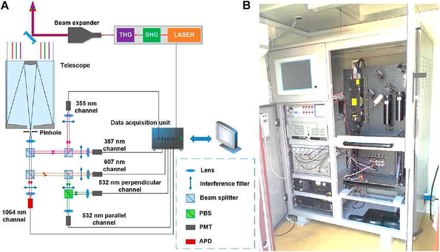
FIGURE 1. (A) MWAL’s structure. (B) MWAL’s cabinet appearance.

The specifications of the MWAL are shown in Table 1.

TABLE 1

TABLE 1. The specifications of MWAL.

Observation Experiments

The MWAL is deployed at the Haidian Park Observation Site (39°59′N, 116°17′E) of the HDMS to conduct all-day operational observations, which can be used to observe and study the spatial and temporal distribution characteristics, optical characteristic parameters and depolarization ratio of atmospheric aerosols and clouds, providing technical support for urban atmospheric environment monitoring and atmospheric pollution research. Figure 2A shows the MWAL at the Haidian Park Observation Site of HDMS, the geographic location of which is shown in Figure 2B. A variety of meteorological elements and atmospheric environment monitoring instruments installed in the HDMS can effectively obtain the data of wind speed, wind direction, temperature, relative humidity, air quality data such as the concentrations of PM_2.5 and PM₁₀. The GTS1 digital radiosonde carried by hydrogen balloon is usually released at 7:15 and 19:15 local time every day to obtain the profiles of the meteorological elements such as temperature, humidity, wind, and pressure. Through the combination of various data, the weather process can be better studied.

FIGURE 2

FIGURE 2. (A) MWAL observed at HDMS. (B) Observation sites of HDMS.

The Principle of Lidar Detection

The lidar equation is the basis for describing the detection principle of lidar and provides the relationship between the lidar echo signal and the optical properties of the measured object. The atmospheric backscattered signal power P(r) at distance r can be determined by the lidar equation [16]:

$P\left(r\right)=\frac{k{P}_0{A}_r\beta \left(r\right)}{r^2}exp\left[-2{\displaystyle \underset{0}{\overset{r}{\int }}\alpha \left(r\prime \right)}dr\prime \right](1)$

where P₀ is the power of the transmitted laser, A_r is the effective receiving area of the telescope, and k is the lidar correction constant, which is related to the geometric overlap factor, the total transmittance, and the range resolution. α(r) and β(r) respectively represent the extinction coefficient and backscattering coefficient of atmospheric molecules and aerosols, which reflect the optical characteristics of the atmosphere. Here, we mainly use the Fernald method [17] to retrieve the optical parameters of aerosols.

The MWAL emits a 532 nm linearly polarized pulsed laser into the atmosphere and the parallel polarization and perpendicular polarization components can be received by two detection channels. Generally, the signal power of the two polarization channels can be described as follows [18].

$P_p\left(r\right)=\frac{k_p{P}_0{A}_r{\beta }_p\left(r\right)}{r^2}\exp \left[-2{\displaystyle \underset{0}{\overset{r}{\int }}\alpha \left(r\prime \right)}dr\prime \right](2)$

$P_s\left(r\right)=\frac{k_s{P}_0{A}_r{\beta }_s\left(r\right)}{r^2}\exp \left[-2{\displaystyle \underset{0}{\overset{r}{\int }}\alpha \left(r\prime \right)}dr\prime \right](3)$

The depolarization ratio δ of atmospheric particles can be defined by the ratio of parallel polarization signal P_p(r) and perpendicular polarization signal P_s(r) as shown in Eq. 4, where K is the calibration factor.

$\delta \left(r\right)=K\frac{P_s\left(r\right)}{P_p\left(r\right)}(4)$

δ is in the range of 0–1, which can be used to study the shape of aerosol particles in the air. The more irregular it is, the larger the depolarization ratio is (such as dust and ice crystals are typical non-spherical particles), while the depolarization ratio of spherical particles (such as water droplets) is relatively small [19, 20]. In a fine and cloudless weather, the depolarization is caused by the atmospheric molecules and δ is about 0.365% for 532 nm [21].

System Calibration Methods and Results

To ensure the accuracy and reliability of the lidar observation, it needs to be calibrated before and during the lidar observation. It mainly includes the correction and gluing of the original data, the collimation of the transmitting and receiving optical axes, the testing of signal saturation, the correction of molecular Rayleigh fitting and the determination of the depolarization ratio correction factor. The corresponding calibration methods are introduced, and the results are discussed.

Data Correction and Gluing

The MWAL uses a six-channel Licel transient recorder as the data collector, and each channel can simultaneously perform analog (AD) mode acquisition and photon counting (PC) mode acquisition with a range resolution of 3.75 m. AD mode has high responsivity to strong echo signals in near-range, while PC mode has higher sensitivity to weak light signals in long-distance. Therefore, gluing the data can effectively improve the signal-to-noise ratio, weak light signal detection capability and signal dynamic range.

Since the AD mode and PC mode in the Licel transient recorder are independent units, the data of the two modes may produce misalignment in the data recording. Therefore, it is necessary to correct the misalignment of data first. Taking the data at 0:00 on 9 September 2019 (local time, the same below) as an example, the signals of clouds from 8 to 9.5 km obtained by the two acquisition modes clearly show that the data collected by the AD mode is lagging the PC mode data (Figure 3A). After comparing the data of the two modes, the AD mode data can be alignment with the PC data by moving the AD data forward by nine points (Figure 3B).

FIGURE 3

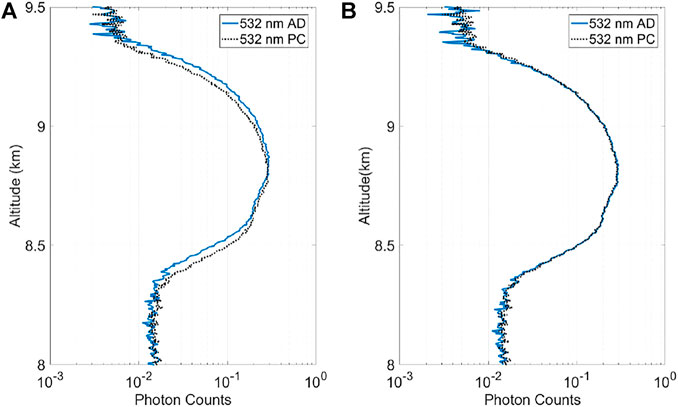
FIGURE 3. (A) The data of AD mode and PC mode before data correction. (B) The data of AD mode and PC mode after data correction.

Then it’s necessary to glue the data collected in the AD mode and the PC mode after correcting the misalignment. Firstly, some proper range with a good linear relationship between AD mode data and PC mode data is selected as the gluing area, and then the coefficients a and b can be obtained by the least square method to convert the AD mode data into PC mode data [22, 23].

${\displaystyle \sum _{i=1}^n{\left(PC\left(i\right)-\left(a\cdot AD\left(i\right)+b\right)\right)}^2}=N_{min}(5)$

where PC(i) is the PC mode data and AD(i) is the AD mode data. The glued data calculated by this method is shown in Figure 4, from which the glued altitude is 2.25 km. Below the glued altitude, the AD mode data has a better response to low-altitude strong signals. While, above the glued altitude, the change trend of the AD mode data and PC mode data is basically consistent. However, with the increase of altitude, PC mode data has a better signal-to-noise ratio than AD mode data. Accordingly, the dynamic range and detection distance of the signal are effectively improved through data gluing.

FIGURE 4

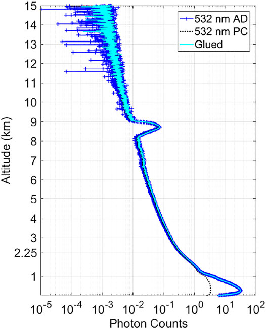
FIGURE 4. The profiles of AD mode data, PC mode data and glued data.

The Collimation of the Transmitting and Receiving Optical Axes

The collimation of the laser transmitting and receiving optical axes is the key to improve the signal receiving efficiency. The MWAL adopts the paraxial mode, that is, the transmitting optical axis is located on one side of the receiving telescope. Therefore, the collimation of the transmitting and receiving optical axes is to make them parallel. Here, we propose a method of signal comparison in the four-quadrant of the telescope to collimate the optical axes. Firstly, the telescope is divided into four quadrants (Figure 5A), and then the echo signals of the left and right quadrants are collected and compared. Adjust the direction of laser emission to make the signals of the left and right quadrants completely consistent. Next, the echo signals of the front quadrant and the back quadrant are collected respectively. Because the distance from the front quadrant to the emitting laser is different from the distance from the back quadrant to the emitting laser, the near-range signals of the two quadrants will be different. However, in the case of the collimation of the transmitting and receiving optical axes, the far-range signals of the two quadrants should be consistent. Consequently, the forward and backward directions of the emitting laser should be adjusted according to the far-range signals. When the optical axes of the transmitting and receiving are aligned using the above method, each quadrant collects data for 1 min. Taking the signal of 532 nm as an example, as shown in Figure 5B, the signals of the left and right quadrants are consistent, and the signals of the four quadrants coincide 1 km away. Below the altitude of 1 km, the signals of the four quadrants are different due to the different distances from the emitted laser to the different quadrants.

FIGURE 5

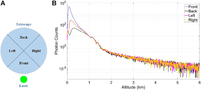
FIGURE 5. (A) Four-quadrant division of the telescope. (B) Comparison of four-quadrant signals after collimation of the transmitting and receiving optical axes.

Signal Saturation Testing

During lidar observation, if the echo signal is saturated, it will lead to signal distortion and even cause damage to the detector. Therefore, it is necessary to test whether there is a problem with signal saturation. Cloudless weather with relatively stable atmospheric conditions is chosen for the test. Firstly, the output laser power is measured and its value is 0.495 W (Q₁) during the lidar observation, and then a group of data accumulated for 1 min is recorded. Secondly, the laser emission power is adjusted by setting different delay time of the Q-Switch of the laser. The average power of the outgoing laser measured by a power meter is 0.413 W (Q₂), 0.335 W (Q₃), 0.273 W (Q₄), 0.213 W (Q₅), 0.14 W (Q₆), and 0.073 W (Q₇) respectively, and the corresponding 6 groups of echo signals accumulated for 1 min are recorded. Taking the signal of 532 nm parallel channel as an example, the 7 groups range corrected signals of 532 nm parallel channels are drawn together in Figure 6A. With the attenuation of laser power, the signal profiles decrease in the same trend. It can be preliminarily judged that there is no saturation phenomenon when the lidar observes with the laser power of Q₁. A method of the linearity test is further used to verify the above inference. Taking the laser power Q₂ to Q₇ as ordinate and the maximum value of the corresponding 6 groups of echo signals as abscissa. A linear fitting line can be drawn, and then we can calculate the deviation between the actual measured value of Q₁ and the value calculated by the fitting line. If the deviation between the calculated value and the measured value of Q₁ is less than 5%, it indicates that the signal linearity is good and the signal is not saturated. If the deviation is greater than 5%, it is necessary to reduce the emission power of the laser for detection, and repeat the above test procedure until it reaches less than 5%.

FIGURE 6

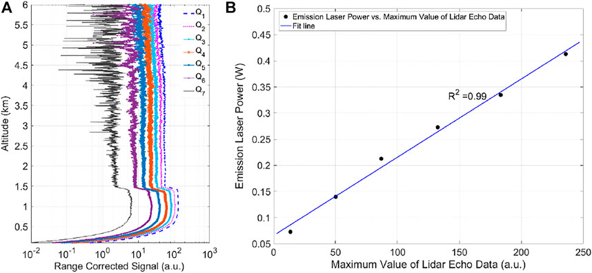
FIGURE 6. (A) The echo signal profiles obtained with different emission laser powers. (B) The fitting line of the emission laser powers and the maximum value of the echo signal profiles.

As shown in Figure 6B, the coefficient of determination R² between the maximum value of the 6 groups of echo signal and emission laser power is 0.99. The calculated value of Q₁ is 0.518 W. Accordingly, the deviation between the calculated value and the measured value of Q₁ is 4.6%, indicating that there is no saturation phenomenon when the lidar observes with the laser power of Q₁.

Molecular Rayleigh Signal Fitting

At the altitudes with aerosols (such as low altitude) or clouds, the signal will be significantly enhanced because of Mie scattering. While at altitudes without aerosols, the lidar echo signal is mainly caused by molecular Rayleigh scattering. The molecular scattering signal obtained by the lidar can be compared with the standard atmospheric molecular Rayleigh signal to further check whether the lidar echo signal is normal [24]. In Figure 7, taking the observation data at 0:00 on 1 June 2021 as an example, the underlying aerosols are mainly distributed below 4.5 km, and clouds exist between 7.2 and 10 km from the range corrected signals of 355 nm, 532, and 1064 nm. The signals of aerosols and clouds are significantly larger than the molecular Rayleigh signals. However, the lidar echo signals of three wavelengths at the altitude between the underlying aerosols and clouds are in good agreement with the standard molecular Rayleigh signals.

FIGURE 7

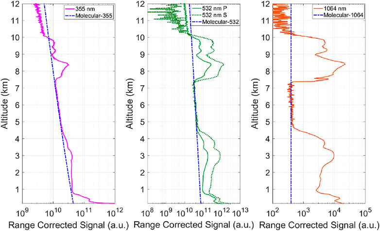
FIGURE 7. Comparison of lidar range corrected signals and molecular Rayleigh signals of 355 nm, 532, and 1064 nm.

Determination of Depolarization Ratio Correction Factor

The correction factor K for calculating the depolarization ratio δ is related not only to the depolarization effect of the lidar system, but also to the detection efficiency of the two detection channels [25]. Therefore, K is one of the important factors to calculate δ. In order to obtain K accurately, a 1/2 wave plate is installed between the laser and the beam expander. A clear day is selected for the determination of K. First, the direction of the optical axis of the 1/2 wave plate is parallel to the laser polarization direction, so that the polarization state of the laser emitted from the wave plate is the same as before. Here the data of the parallel polarization channel and perpendicular polarization channel are recorded as P1 and S1 respectively. Then the 1/2 wave plate is rotated so that the angle between the optical axis direction of the 1/2 wave plate and the laser polarization direction is 45°. The laser outgoing from the wave plate is still linearly polarized, and the angle between the polarization direction of the outgoing laser and the polarization direction of the original incident laser is 90°. In this case the data of the two polarization channels are recorded as P2 and S2 respectively. After subtracting the background from P1 and S2, a region where both signals are smooth is selected and the K is approximately 1.65 calculated by P1/S2 (as shown in Figure 8A). In addition, δ of atmospheric molecules (approximately 0.365%) and high-altitude cirrus clouds (30%–80%) can be used to further test and revise the K [26]. As shown in Figure 8B, the lidar observation data at 19:15 on 20 June 2019 is compared and analyzed with the potential temperature and relative humidity profiles of the digital radiosonde (Figure 8C). Through the lidar echo signal profile, the aerosols are mainly distributed below 5 km, which is consistent with the altitude of the maximum gradient absolute value of relative humidity and potential temperature. The lower δ below 5 km is probably due to the higher relative humidity. The main components of the atmosphere from 6 to 10.5 km are atmospheric molecules, and δ is relatively small. The cirrus clouds are distributed from 10.5 to 13 km with a δ higher than 0.4, where the potential temperature changes slowly and the relative humidity is lower than 15%, indicating that the cirrus clouds are mainly composed of ice crystals.

FIGURE 8

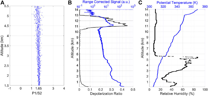
FIGURE 8. (A) Correction factor K. (B) The profiles of range corrected signal and depolarization ratio at 19:15 on 20 June 2019. (C) The profiles of potential temperature and relative humidity at 19:15 on 20 June 2019.

Observation Example Analysis of a Haze Process

After the lidar is calibrated, it can better serve the monitoring of the atmospheric environment. Using the joint analysis of lidar and other meteorological data, the weather process can be better analyzed, and the performance of the lidar can be further tested. Taking a haze process in Beijing from 29 September to 2 October 2019 as an example, the weather process, temporal and spatial distribution, and possible sources of the haze are studied through the analysis of multiple observations data.

Comparative Analysis of Lidar and Digital Radiosonde Data

From 29 September to 2 October 2019, the MWAL observed a haze process in Beijing. From the time-height-indication (THI) figure of the range corrected signal of 532 nm in Figure 9A, the aerosols are mainly distributed below 3 km and the haze is heaviest on 30 September. From the THI figure of extinction coefficient (Figure 9B), we can see that the extinction coefficient near the ground is higher and haze occurs a similar diurnal change trend in these 4 days. The concentration of aerosols near-ground gradually increases after 0:00, and so does the haze thickness. The height and concentration of haze gradually decrease in the afternoon.

FIGURE 9

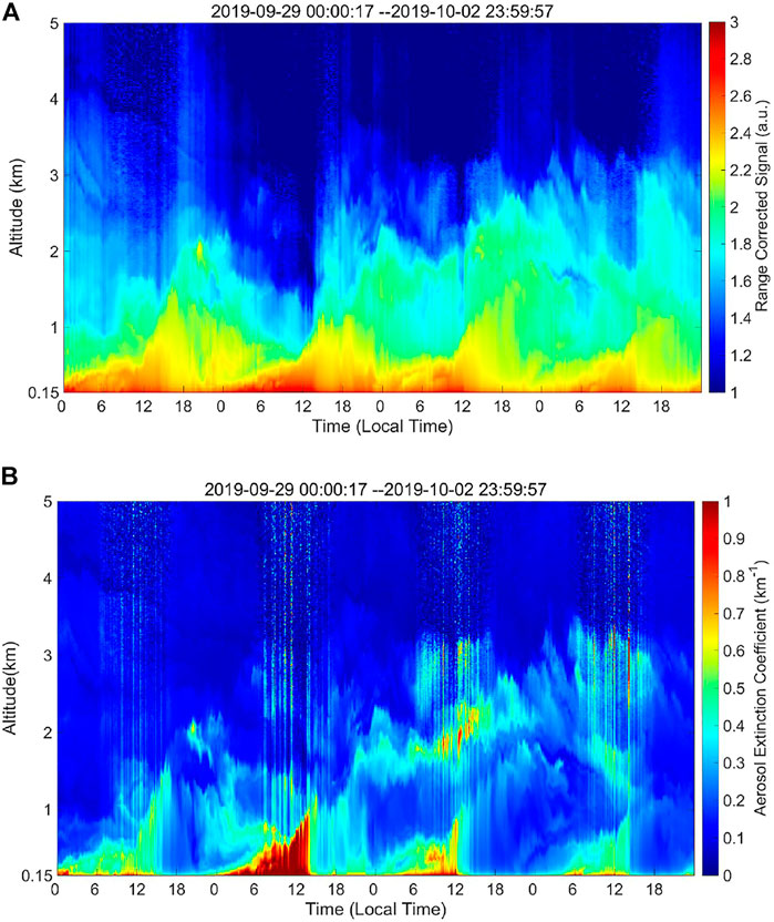
FIGURE 9. (A) THI figure of range corrected signal at 532 nm from 29 September to 2 October 2019. (B) THI figure of extinction coefficient at 532 nm from 29 September to 2 October 2019.

Taking the weather process on 1 October as an example, the lidar observation data and the digital radiosonde data at three moments are used for analysis. The potential temperature and relative humidity profiles at 7:15, 13:15, and 19:15 on 1 October (Figure 10A) show that the relative humidity is approaching or exceeding 80% and the potential temperature changes slowly at the altitude from 1.5 to 3.5 km. The changing trend of the extinction coefficient profiles in altitude at three times (Figure 10B) is consistent with that of the relative humidity. The altitude of the maximum absolute value of the aerosol extinction coefficient gradient is the same with the altitude of the maximum absolute value of the potential temperature and relative humidity gradient, indicating the thickness of the haze. At the altitude of 1.5–3.5 km, the increase of relative humidity may lead to an increase of hygroscopic growth of aerosol particles and an increase of aerosols extinction coefficient.

FIGURE 10

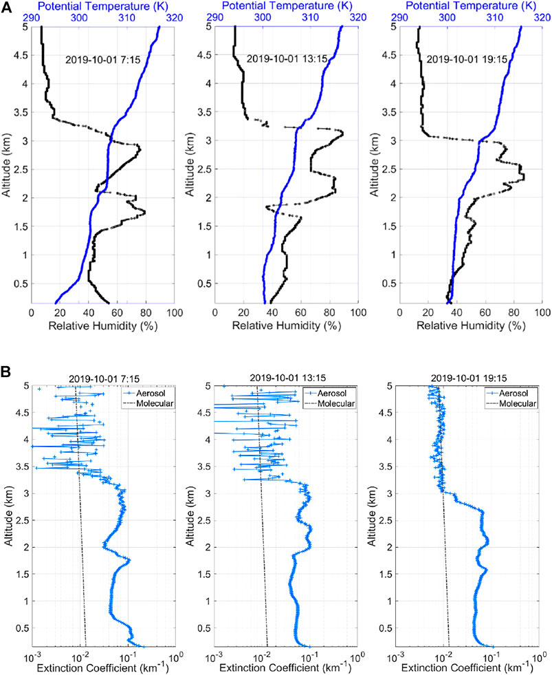
FIGURE 10. (A) The profiles of potential temperature and relative humidity at 7:15, 13:15, and 19:15 on 1 October 2019. (B) The profiles of extinction coefficient at 7:15, 13:15, and 19:15 on 1 October 2019.

Analysis of Ground Observation Data

In order to better analyze the air quality situation near the ground, we can clearly see the changes of the PM_2.5 and PM₁₀ concentrations recorded by the air quality monitor from 29 September to 2 October 2019 (Figure 11). The concentrations of PM₁₀ are all higher than 100 μg/m³, with the higher PM₁₀ concentration during the daytime on 30 September, and the highest value of 252 μg/m³ at 14:00. The concentration of PM_2.5 reaches a maximum value of 110.6 μg/m³ at 14:00 on 2 October. Figure 12 shows the ratio of PM_2.5/PM₁₀ is more than 80% at this moment. The ratio of PM_2.5/PM₁₀ at other time is basically less than 50%, indicating that the haze is mainly caused by PM₁₀ pollutants, which should be caused by the transportation of urban floating dust.

FIGURE 11

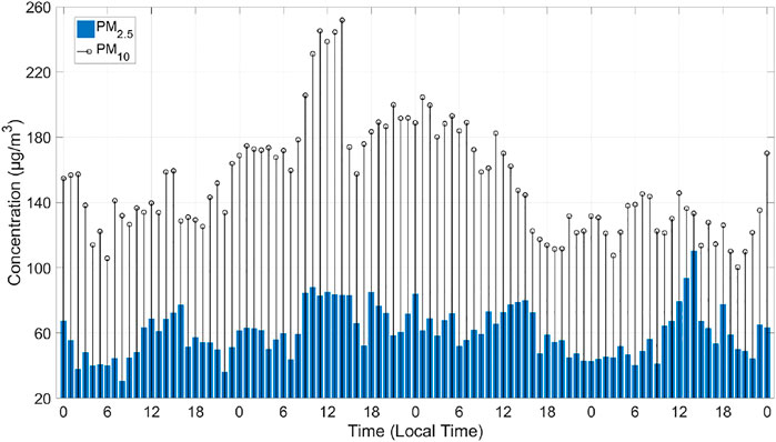
FIGURE 11. Air quality monitoring data.

FIGURE 12

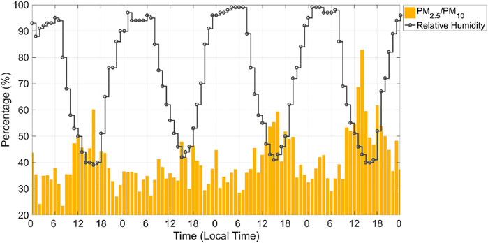
FIGURE 12. Variation curves of ground relative humidity and PM_2.5/PM₁₀.

As shown in Figure 12, during the observation period from 29 September to 2 October 2019, the relative humidity changes regularly. Generally, the relative humidity is high at night, and decreases during the daytime due to the variation of temperature. The relative humidity is basically above 90% from 0:00 to 6:00, and close to 100% from 0:00 to 6:00 on 1 and 2 October. High relative humidity will cause the hygroscopic growth and the sedimentation of aerosol particles, so the aerosols extinction coefficient observed by lidar at night is relatively low. It can be seen from Figure 12 that there is a negative correlation between relative humidity and PM_2.5/PM₁₀, that is, when the relative humidity is high, the proportion of PM_2.5 is relatively low.

HYSPLIT Trajectory Analysis

The ground meteorological data recorded by HDMS show that the south wind class 1 to 2 is dominant during this period, indicating thar the aerosols is mainly transported by the south wind and there is a lack of good diffusion conditions. The NOAA HYSPLIT trajectory model can support the source analysis of this haze. Taking the Haidian Park observation site of HDMS as the reference location, the backward trajectory of aerosols at different altitudes could be tracked. As shown in Figure 13A, the aerosols at the altitudes of 100, 300, and 500 m at 8:00 Beijing time on 30 September 2019, mainly come from near ground aerosols of Hebei and Shandong provinces to the south of Beijing. From Figure 13B, at 10:00 Beijing time on 1 October 2019, the aerosols at 100, 300, and 500 m also mainly originated from the near-ground of the south of Beijing.

FIGURE 13

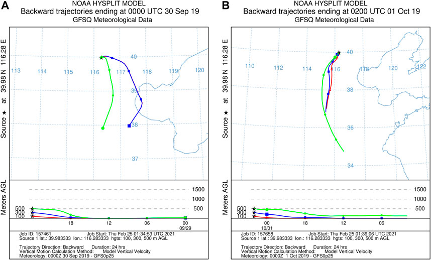
FIGURE 13. (A) Backward trajectories of aerosols at the altitudes of 100, 300, and 500 m at 8:00 on 30 September 2019, Beijing time. (B) Backward trajectories of aerosols at the altitudes of 100, 300, and 500 m at 10:00 on 1 October 2019, Beijing time.

Conclusion

A multi-wavelength aerosol lidar is carrying out an observation campaigns in HDMS of Beijing. The contents and methods of regular calibration of lidar are discussed, mainly including the correction and gluing of the original data, the collimation of the transmitting and receiving optical axes, the testing of signal saturation, the correction of molecular Rayleigh fitting and the determination of the depolarization ratio correction factor. All these can be used for the regular calibration of lidar operational observation to ensure the accuracy and reliability of the observed data. Finally, a haze process from 29 September to 2 October 2019 is analyzed by using the data of lidar, digital radiosonde, air quality and relative humidity of HDMS. The observation results show that the increase of extinction coefficient near the ground indicates the occurrence of haze phenomenon and the haze is most serious on 30 September. Comparing the profiles of potential temperature and relative humidity with the extinction coefficient profiles at three times on 1 October, it is found that the changing trend of the aerosol extinction coefficient in altitude is consistent with that of the relative humidity. High relative humidity will cause hygroscopic growth and the sedimentation of aerosol particles. Using the PM_2.5 and PM₁₀ data recorded by the air quality monitor, it is analyzed that the haze is mainly caused by PM₁₀ pollutants and the PM_2.5/PM₁₀ has a negative correlation relation with the relative humidity. It can be inferred that pollutants should be caused by the transportation of urban floating dust. The aerosols mainly originated from the near-ground of the south of Beijing by the analysis of NOAA’s HYSPLIT trajectory model.

Data Availability Statement

The raw data supporting the conclusions of this article will be made available by the authors, without undue reservation.

Author Contributions

CC, XS, and ZW designed the research, YC, XUW (XOW), XZ and XP performed the experiments, ZB, QZ, HL, FZ, and XL analyzed the data, XOW (XUW) and RZ proposed the methods, CC and XS wrote the paper.

Funding

This work is jointly supported by the following project grants: National Key Research and Development Program of China (2021YFB3901304), Key Research and Development Plan of Shandong Province (2020CXGC010104), Development Fund Project of Institute of Oceanographic Instrumentation, Shandong Academy of Sciences (HYPY202106), Guangdong basic and Applied basic Research Fund (2020B1515120056), Qingdao Pilot National Laboratory for Marine Science and Technology (2021WHZZB0205and2021WHZZB1500) and International Cooperation Project of Shandong Academy of Sciences (2019GHZD02).

Conflict of Interest

Authors CC and ZW were employed by Shandong SCICOM Shenguang Technology Co., Ltd.

The remaining authors declare that the research was conducted in the absence of any commercial or financial relationships that could be construed as a potential conflict of interest.

Publisher’s Note

All claims expressed in this article are solely those of the authors and do not necessarily represent those of their affiliated organizations, or those of the publisher, the editors and the reviewers. Any product that may be evaluated in this article, or claim that may be made by its manufacturer, is not guaranteed or endorsed by the publisher.

Acknowledgments

Special thanks to CMA Meteorological Observation Centre and Haidian District Meteorological Service of Beijing for providing observational support for multi-wavelength aerosol lidar and data support for digital radiosonde and ambient air quality monitoring, etc. The authors gratefully acknowledge the NOAA Air Resources Laboratory (ARL) for the provision of the HYSPLIT transport and dispersion model and/or READY website used in this publication.

References

1. Zhang Y, Zhang Y, Yu C, Yi F. Evolution of Aerosols in the Atmospheric Boundary Layer and Elevated Layers during a Severe, Persistent Haze Episode in a Central China Megacity. Atmosphere (2021) 12(2):152. doi:10.3390/atmos12020152

CrossRef Full Text | Google Scholar

2. Lang Z, Qiao S, Ma Y. Acoustic Microresonator Based In-Plane Quartz-Enhanced Photoacoustic Spectroscopy Sensor with a Line Interaction Mode. Opt Lett (2022) 47(6):1295–8. doi:10.1364/OL.452085

PubMed Abstract | CrossRef Full Text | Google Scholar

3. Cheng B, Ma Y, Feng F, Zhang Y, Shen J, Wang H, et al. Influence of Weather and Air Pollution on Concentration Change of PM2.5 Using a Generalized Additive Model and Gradient Boosting Machine. Atmos Environ (2021) 255:118437. doi:10.1016/j.atmosenv.2021.118437

CrossRef Full Text | Google Scholar

4. Wu J, Zhang Y, Wang T, Qian Y. Rapid Improvement in Air Quality Due to Aerosol-Pollution Control during 2012-2018: An Evidence Observed in Kunshan in the Yangtze River Delta, China. Atmos Pollut Res (2020) 11:693–701. doi:10.1016/j.apr.2019.12.020

CrossRef Full Text | Google Scholar

5. Chen C, Song X, Wang Z, Wang W, Wang X, Zhuang Q, et al. Observations of Atmospheric Aerosol and Cloud Using a Polarized Micropulse Lidar in Xi'an, China. Atmosphere (2021) 12:796. doi:10.3390/atmos12060796

CrossRef Full Text | Google Scholar

6. Chang L, Li J, Chu Y, Dong Y, Tan W, Xu X, et al. Variability of Surface Aerosol Properties at an Urban Site in Beijing Based on Two Years of In-Situ Measurements. Atmos Res (2021) 256:105562. doi:10.1016/j.atmosres.2021.105562

CrossRef Full Text | Google Scholar

7. Ma Y, He Y, Tong Y, Yu X, Tittel FK. Quartz-tuning-fork Enhanced Photothermal Spectroscopy for Ultra-high Sensitive Trace Gas Detection. Opt Express (2018) 26(24):32103–10. doi:10.1364/OE.26.032103

PubMed Abstract | CrossRef Full Text | Google Scholar

8. Kim D, Ramanathan V. Solar Radiation Budget and Radiative Forcing Due to Aerosols and Clouds. J Geophys Res (2008) 113:D02203. doi:10.1029/2007JD008434

CrossRef Full Text | Google Scholar

9. Rader F, Traversi R, Severi M, Becagli S, Müller K-J, Nakoudi K, et al. Overview of Aerosol Properties in the European Arctic in Spring 2019 Based on In Situ Measurements and Lidar Data. Atmosphere (2021) 12:271. doi:10.3390/atmos12020271

CrossRef Full Text | Google Scholar

10. Liu D, Yang Y, Cheng Z, Huang H, Zhang B, Ling T, et al. Retrieval and Analysis of a Polarized High-Spectral-Resolution Lidar for Profiling Aerosol Optical Properties. Opt Express (2013) 21:13084–93. doi:10.1364/OE.21.013084

PubMed Abstract | CrossRef Full Text | Google Scholar

11. Yorks JE, Selmer PA, Kupchock A, Nowottnick EP, Christian KE, Rusinek D, et al. Aerosol and Cloud Detection Using Machine Learning Algorithms and Space-Based Lidar Data. Atmosphere (2021) 12:606. doi:10.3390/atmos12050606

CrossRef Full Text | Google Scholar

12. Ma Y, Feng W, Qiao S, Zhao Z, Gao S, Wang Y. Hollow-core Anti-resonant Fiber Based Light-Induced Thermoelastic Spectroscopy for Gas Sensing. Opt Express (2022) 30(11):18836–44. doi:10.1364/OE.460134

CrossRef Full Text | Google Scholar

13. Yu S, Liu D, Xu J, Wang Z, Wu D, Shan Y, et al. Optical Properties and Seasonal Distribution of Aerosol Layers Observed by Lidar over Jinhua, Southeast China. Atmos Environ (2021) 257:118456. doi:10.1016/j.atmosenv.2021.118456

CrossRef Full Text | Google Scholar

14. Pisani G, Boselli A, Coltelli M, Leto G, Pica G, Scollo S, et al. Lidar Depolarization Measurement of Fresh Volcanic Ash from Mt. Etna, Italy. Atmos Environ (2012) 62:34–40. doi:10.1016/j.atmosenv.2012.08.015

CrossRef Full Text | Google Scholar

15. Cao X, Wang Z, Tian P, Wang J, Zhang L, Quan X. Statistics of Aerosol Extinction Coefficient Profiles and Optical Depth Using Lidar Measurement over Lanzhou, China since 2005-2008. J Quantitative Spectrosc Radiative Transfer (2013) 122:150–4. doi:10.1016/j.jqsrt.2012.09.016

CrossRef Full Text | Google Scholar

16. Wang Z, Mao J, Li J, Zhao H, Zhou C, Sheng H. Six-channel Multi-Wavelength Polarization Raman Lidar for Aerosol and Water Vapor Profiling. Appl Opt (2017) 56:5620–9. doi:10.1364/AO.56.005620

PubMed Abstract | CrossRef Full Text | Google Scholar

17. Fernald FG. Analysis of Atmospheric Lidar Observations: Some Comments. Appl Opt (1984) 23:652–3. doi:10.1364/AO.23.000652

PubMed Abstract | CrossRef Full Text | Google Scholar

18. Xian J, Sun D, Xu W, Tian C, Tan Q, Han Y, et al. Calibration and Calculation of Polarization Lidar. Earth Space Sci (2019) 6:1161–70. doi:10.1029/2019EA000609

CrossRef Full Text | Google Scholar

19. Liu L, Mishchenko MI. Spectrally Dependent Linear Depolarization and Lidar Ratios for Nonspherical Smoke Aerosols. J Quantitative Spectrosc Radiative Transfer (2020) 248:106953. doi:10.1016/j.jqsrt.2020.106953

CrossRef Full Text | Google Scholar

20. Wu S, Song X, Liu B, Dai G, Liu J, Zhang K, et al. Mobile Multi-Wavelength Polarization Raman Lidar for Water Vapor, Cloud and Aerosol Measurement. Opt Express (2015) 23:33870–92. doi:10.1364/OE.23.033870

PubMed Abstract | CrossRef Full Text | Google Scholar

21. Alvarez JM, Vaughan MA, Hostetler CA, Hunt WH, Winker DM. Calibration Technique for Polarization-Sensitive Lidars. J Atmos Ocean Tech (2006) 23:683–99. doi:10.1175/JTECH1872.1

CrossRef Full Text | Google Scholar

22. Zhang Y, Yi F, Kong W, Yi Y. Slope Characterization in Combining Analog and Photon Count Data from Atmospheric Lidar Measurements. Appl Opt (2014) 53:7312–20. doi:10.1364/AO.53.007312

PubMed Abstract | CrossRef Full Text | Google Scholar

23. Gao F, Veberič D, Stanič S, Bergant K, Hua D-X. Performance Improvement of Long-Range Scanning Mie Lidar for the Retrieval of Atmospheric Extinction. J Quantitative Spectrosc Radiative Transfer (2013) 122:72–8. doi:10.1016/j.jqsrt.2012.11.027

CrossRef Full Text | Google Scholar

24. Bucholtz A. Rayleigh-scattering Calculations for the Terrestrial Atmosphere. Appl Opt (1995) 34:2765–73. doi:10.1364/AO.34.002765

PubMed Abstract | CrossRef Full Text | Google Scholar

25. Wang L, Stanič S, Eichinger W, Song X, Zavrtanik M. Development of an Automatic Polarization Raman Lidar for Aerosol Monitoring over Complex Terrain. Sensors (2019) 19:3186. doi:10.3390/s19143186

PubMed Abstract | CrossRef Full Text | Google Scholar

26. Chen W-N, Chiang C-W, Nee J-B. Lidar Ratio and Depolarization Ratio for Cirrus Clouds. Appl Opt (2002) 41:6470–746. doi:10.1364/AO.41.006470

PubMed Abstract | CrossRef Full Text | Google Scholar