Multivariate statistical modelling to improve particle treatment verification: Implications for prompt gamma-ray timing

We present an improved method for in-vivo proton range verification by prompt gamma-ray timing based on multivariate statistical modelling. To this end, prompt gamma-ray timing distributions acquired during pencil beam irradiation of an acrylic glass phantom with air cavities of different thicknesses were analysed. Relevant distribution features were chosen using forward variable selection and the Least Absolute Shrinkage and Selection Operator (LASSO) from a feature assortment based on recommendations of the Image Biomarker Standardisation Initiative. Candidate models were defined by multivariate linear regression and evaluated based on their coefficient of determination R² and root mean square error RMSE. The newly developed models showed a clearly improved predictive power (R² > 0.7) compared to the previously used models (R² < 0.5) and allowed for the identification of introduced air cavities in a scanned treatment field. These results demonstrate that elaborate statistical models can enhance prompt gamma-ray based treatment verification and increase its potential for routine clinical application.

1 Introduction

Compared to conventional photon-based radiotherapy, proton therapy offers the advantage of a pronounced dose maximum at the Bragg peak, which can be tailored to a predefined tumour volume while sparing healthy tissue behind the tumour [1]. However, the steep gradient of this peak and the dependence of its position on the traversed material in the patient make the dose distribution very sensitive to inter- and intrafractional uncertainties resulting from setup errors and anatomical variations [2]. These uncertainties currently translate into restrictions in the applicable beam angles and treatable tumour sites, as well as into safety margins around the tumour, which can limit treatment efficacy. Although pretreatment image guidance (e.g. in-room or on-board cone-beam computed tomography) is becoming more accessible, this approach may cause additional dose to the patient and interrupt the treatment workflow. Also, it cannot fully account for intrafractional motion and deformation, which can be especially relevant for moving tumours e.g., in the thorax and abdomen region [3].

A complimentary strategy to reduce these uncertainties is on-line monitoring of secondary radiation generated in the patient during irradiation. The spatial, temporal and energy distributions of prompt gamma-rays have been shown to correlate strongly with the Bragg peak position in the patient [4]. As a light-weight, collimator-free technique, that can be easily integrated into existing systems, prompt gamma-ray timing (PGT) [5] has gained increasing interest for this purpose in recent years [6–8]. A longer proton range translates into a longer time-of-flight of the particles. Therefore, the temporal distribution of prompt gamma-rays measured with scintillation detectors can be used to reconstruct the delivered proton range in the patient.

However, the uncertainty in the range reconstructed with this method is still more than 5 mm at 5,000 processed gamma rays [6]. One of the main reasons for this is seen in the range reconstruction method, which is currently based on a simple univariate linear regression of either the mean or the standard deviation of the timing distributions. Yet, timing distributions acquired with differing material compositions exhibit complex shape changes, such as dips and changes in curvature, which are not sufficiently represented by the mean and standard deviation (cf. Figure 2).

Therefore, the aim of this work is to develop an improved reconstruction method that is capable of increasing the precision of proton range prediction for the prompt gamma-ray timing method and transferable to other range verification methods. The presented approach is based on a standardised distribution feature assortment, out of which strongly predictive parameters are objectively selected and combined to multivariate regression models. The method is introduced in the following section, validated and compared against the current method in section 3 and conclusively discussed in section 4.

2 Material and methods

2.1 Experimental setup

The data used for this study were taken from measurements described in detail by Werner et al. [6, 9]. The setup is depicted schematically in Figure 1. A homogeneous cylindrical phantom comprised of poly(methyl methacrylate) was used (PMMA, acrylic glass, ${[{\mathrm{C}}_5{\mathrm{O}}_2{\mathrm{H}}_8]}_{\text{n}}$). Air cavities of varying thickness ΔR ∈ {0 mm, 5 mm, 10 mm, 20 mm} were successively introduced into the phantom to mimic anatomical variations leading to range deviations. For each air cavity thickness, the phantom was irradiated with proton pencil beams of two different kinetic energies (E₁ = 162 MeV and E₂ = 227 MeV) and a micropulse repetition rate of 106.3 MHz. Prompt-gamma ray timing distributions were measured with a detection unit consisting of a ∅ 2″×2″ CeBr₃ crystal by Scionix¹, a Hamamatsu² R13089-100 photomultiplier and a U100 digital spectrometer by Target Systemelektronik³, which was placed at a backward angle of 130° [6]. Two experiments were performed with different beam characteristics:

FIGURE 1

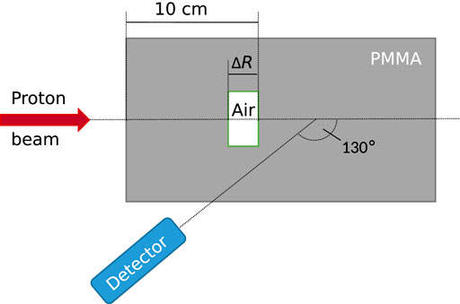
FIGURE 1. Schematic representation of the experimental setup. A proton beam impinged on a polymethyl methacrylate (PMMA) phantom with air cavities of varying thickness. Emitted gamma rays were measured under a backward angle of 130°. The detector axis crossed the beam axis at a depth of half the proton range. Details on the experiment can be found in [6].

Static beam experiment: In a first experiment, a static pencil beam was directed centrally at the phantom. The beam was pulsed in spots with a spot duration of 69 ms, a period of 72 ms and 10⁹ protons per spot⁴. One measurement consisted of 100 spots. The data of the first 30 spots were omitted due to the phase oscillation effect [6].

Scanning experiment: In a second experiment, pencil beam scanning was applied [9]. For each measurement, the distal energy layer of a treatment plan homogeneously irradiating a cubic volume of 8 × 8 × 8 cm³ was applied. The layer contained 225 pencil beam spots corresponding to 225 scanning positions, and the number of protons per spot ranged between 1 × 10⁸ in the centre of the layer (corresponding to a clinical pencil beam scanning spot weight) and 4 × 10⁸ at the field edges. The energy layer was repeated eight times per measurement to simulate the counting statistics acquired by a PGT system consisting of eight detectors.

Each of the two experiments comprised eight measurements covering the set of four cavity thicknesses ΔR and two beam energies E₁ and E₂. The system was operated approximately at a detector trigger count rate of 500 kcps, a dead time of 1 µs per event, a pile up probability of 5%, and a proton beam current at nozzle exit of 2 nA.

2.2 Data preprocessing

The raw data of each measurement was preprocessed following the method established in [6]: The photomultiplier gain drift and time digitalisation non-linearities were corrected for, the integral signal charge was converted into deposited energy and all events with an energy deposition below 3 MeV or above 5 MeV were discarded. For the remaining events, the detection time relative to the accelerator radiofrequency was used to populate spot-wise PGT histograms h(t_i). The histograms had a bin width of 4.6 ps (i.e., the accelerator period of 9.4 ns divided by 2048) and a mean event count of approximately 5,000 events per spot for the static beam experiment and 500–2,000 events per spot for the scanning experiment. Finally, the long-term time-dependent phase shift was corrected for and background events were removed, as detailed in Supplementary Section S1. An example of the preprocessed histograms h(t_i) is depicted in Figure 2.

FIGURE 2

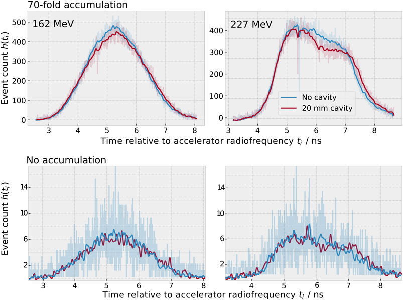
FIGURE 2. Measured prompt gamma-ray timing spectra h(t_i) for an initial proton beam energy of 162 MeV (left) and 227 MeV (right) for the static beam experiment after preprocessing. Top: When adding a 20 mm cavity (red), less prompt gamma-rays are produced in the cavity and longer times of flight are more probable than in the case without cavity (blue). For better visibility, the data of seventy static spots were accumulated and smoothed with a Gaussian filter (σ = 5 bins) for this graph. The unsmoothed data are underlaid semi-transparently. Bottom: Data of a single spot (without accumulation). The unsmoothed data of single spots was used for analysis. The histogram bin width was 4.6 ps

2.3 Model generation

The data of the static beam experiment was split into a training dataset of 50 spots per measurement and a validation dataset of 20 spots per measurement. The training dataset was used for model generation.

First, the two models presented by Werner et al. [6] were reproduced to enable a comparison with the newly developed models. These two models were generated by a univariate linear regression of either the mean or the standard deviation of the timing histograms as regressor and the cavity thickness ΔR as dependent variable.

The new multivariate models were generated in three steps: parameter definition, parameter selection and multivariate linear regression. This process was performed three times: once for the dataset of each proton energy separately (energy-specific models) and once for both proton energies combined (energy-overarching models). The model generation process is depicted in Figure 3.

FIGURE 3

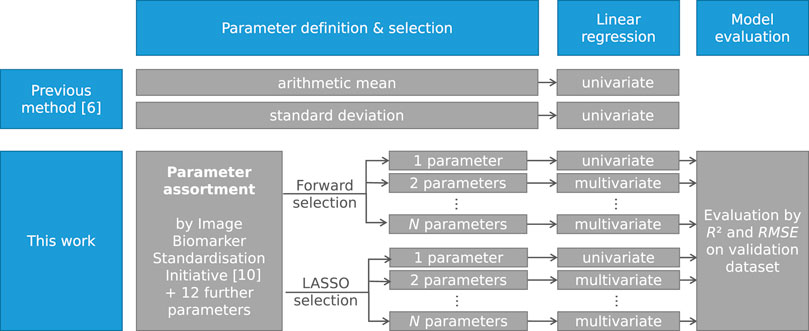
FIGURE 3. Schematic representation of the model generation process as applied by Werner et al. [6] and as presented in this work. The process was repeated for each individual proton energy and for both proton energies combined.

2.3.1 Parameter definition

The aim of the parameter definition is to generate a broad and varied parameter assortment out of which independent, highly predictive features can be selected by selection algorithms in the next step. For this, an assortment of 23 parameters was used, following the recommendations of the Image Biomarker Standardisation Initiative for one-dimensional histograms (see [10], Section 3.4, and Supplementary Section S2). The following parameters were added to this assortment:

• the area under the curve, as defined by the sum of all histogram entries ∑_ih(t_i),

• the T1-to-T2 distance, as defined by Marcatili et al. [11],

• the standard deviation of the histogram σ(t_i),

• the position of the fall-off of the distribution, as defined by the highest negative slope of the histogram curve (in a moving interval of 64 bins width),

• five further interquantile ranges F_iqn = P_b − P_a, where P_a and P_b are the ath and bth percentile of the times t_i, respectively, and (a, b) ∈ {(20, 80), (30, 70), (35, 65), (40, 60), (50, 90)},

• two further robust mean absolute deviations, i.e. the mean absolute deviations between two percentiles P_a and P_b, where (a, b) ∈ {(20, 80), (50, 90)}, and

• one additional quantile coefficient of dispersion $F_{\mathrm{qncod}}=\frac{P_a-P_b}{P_a+P_b}$, where (a, b) = (35, 65).

The addition of these parameters was motivated as follows. When adding a cavity, longer times of flight are more probable than in the case without cavity (cf. Figure 2). As a result, the position of the fall-off increases and was therefore added to the parameter assortment. The same process leads to an increase in the width of the distribution. Since it is a priori not clear which measure of the width is most predictive, four symmetric interquartile ranges as well as a further symmetric robust mean absolute deviation and quantile coefficient of dispersion were added. The T1-to-T2-distance was defined in [11] as a further measure of the distribution width. A second physical effect is the reduced gamma-ray yield in the cavity. This leads to a dip in the PGT distribution, as visible in the right half of the timing distribution for 227 MeV (see Figure 2). For this reason, the asymmetric interquartile range and robust mean absolute deviation describing the right half of the distribution (50–80%) were added. Furthermore, the peak intensity is reduced, which motivated the inclusion of the area under the curve.

Three parameters suggested in [10] were excluded in this work since they were constant for all timing histograms h(t_i): the minimum discretised intensity (min(t_i) = 0 ns), the maximum discretised intensity (max(t_i) = 9.4 ns), and the discretised intensity range (max(t_i)–min(t_i) = 9.4 ns). Furthermore, the maximum and minimum histogram gradients h(t_i) − h(t_i+1) and their respective intensity were excluded from analysis, since these highly local parameters are dominated by statistical noise (see Figure 2, bottom row). The remaining parameter assortment comprised 28 parameters, as listed in Supplementary Section S2. For all parameters, the p-value of univariate linear regression and the Pearson correlation matrix were calculated.

2.3.2 Parameter selection

To generate a model with high predictive power for the proton range based on a reduced subset of the 28 considered parameters, two established parameter selection methods were compared (see Supplementary Figure S8 in Supplementary Information):

Forward variable selection: Forward variable selection is an iterative method that successively adds the parameter with the highest p-value of multivariate linear regression to the selected parameter set in each iteration step [12]. An inclusion p-value of p = 0.2 was used to ensure that enough parameters are included. The N_sel selected parameters were ranked according to their importance using the number of the iteration step during which they were added, a lower rank indicating a higher importance.

LASSO method: The LASSO (Least Absolute Shrinkage and Selection Operator) method optimises the number of parameters during multivariate regression by minimising the sum of squared differences and an additional penalty term (λ ⋅∑|β_j|) consisting of the sum of the regression coefficients β_j and the regularisation penalty λ [13].

The parameters were standardised by subtracting the mean and dividing by the standard deviation. λ was defined by fourfold cross validation, i.e., the training dataset was split into four subsets to find and validate an optimal λ. Histogram parameters with a coefficient of zero were discarded. The remaining N_sel parameters were ranked by their absolute regression coefficient, i.e., the parameter with the highest absolute coefficient was assigned the lowest rank.

For both methods, N = min{N_max, N_sel} parameter sets were generated. Each parameter set consisted of the n parameters with the lowest rank, where n ∈ {1, 2, … , N}. For example, if two parameters were selected (N_sel = 2), two parameter sets were generated (N = 2): One including only the parameter with the lowest rank (n = 1), and one including the two parameters with the two lowest ranks (n = 2). This way, the model performance could be analysed as a function of the number of included parameters. N_max was set to 20 as an upper limit for the number of parameters per model.

To evaluate the efficacy of the parameter selection, one hundred further parameter sets were generated based on a random choice of three parameters per model from the parameter assortment. One further parameter set was defined containing both the arithmetic mean and the standard deviation, which were used only individually in [6].

2.3.3 Regression

For each parameter, the Pearson and Spearman correlation with the cavity thickness were compared. Since no relevant differences were found, the data was assumed to mainly correlate linearly. Thus, models were defined by multivariate linear regression of the n selected parameters as regressors and the cavity thickness ΔR as dependent variable.

2.4 Evaluation

The last 20 spots of the static beam experiment were used for model validation. The validation was performed by comparing the cavity thickness predicted by the models from the timing histograms to the actual cavity thickness in the phantom. This was done quantitatively by calculating the respective coefficient of determination R² and the root mean square error RMSE. The performance of the different models was compared and the most often selected histogram parameters were identified.

To assess the capability of the models to detect air cavities in a scanned treatment field, difference maps between the predicted range of the reference measurement and the measurements with air cavities of the scanning experiment were generated for all models. The smoothing filter proposed in [6] was applied. The analysis was performed once without accumulation and once accumulating the data of all eight repetitions to mimick the number of events acquired by a prompt gamma-ray timing system consisting of eight detectors. The scanned beam data was rated qualitatively by comparing the visibility of the air cavity in the range difference maps reconstructed with the old and new models. The RMSE between actual and predicted range deviation was compared between the models for the five central scanning spots.

The programming language used for this work was python (version 3.9.7) and its associated modules [14]. The model generation was based on the statsmodels and the scikit-learn module (versions 0.12.2 and 0.24.2, respectively).

3 Results

3.1 Selected distribution parameters

The ranking of the selected parameters is depicted in Supplementary Section S4 and the four most important parameters are summarised for each model in Table 1. The following observations can be made: 1) Most of the selected parameters refer to the width of the distribution (T1-to-T2-distance, median absolute deviation, variance, robust mean absolute deviation, interquartile range). This behaviour is consistent with the fact that a longer path length introduced by the air cavities leads to longer times of flight. 2) For the higher energy (227 MeV), the two selection methods showed a very high agreement and the second half of the timing distribution gained importance, as expressed by the robust mean absolute deviation (50–90%) and the 90th percentile. For this energy, a dip in the second half of the timing distribution is present, as less gamma rays are produced in the air cavity (see Figure 2). 3) For the energy-overarching model, parameters that are normalised appeared to be of high relevance to account for the energy-specific variability in the distributions. This behaviour was expressed in the selection of the quartile coefficient of dispersion and the coefficient of variation, but only for the forward variable selection method.

TABLE 1

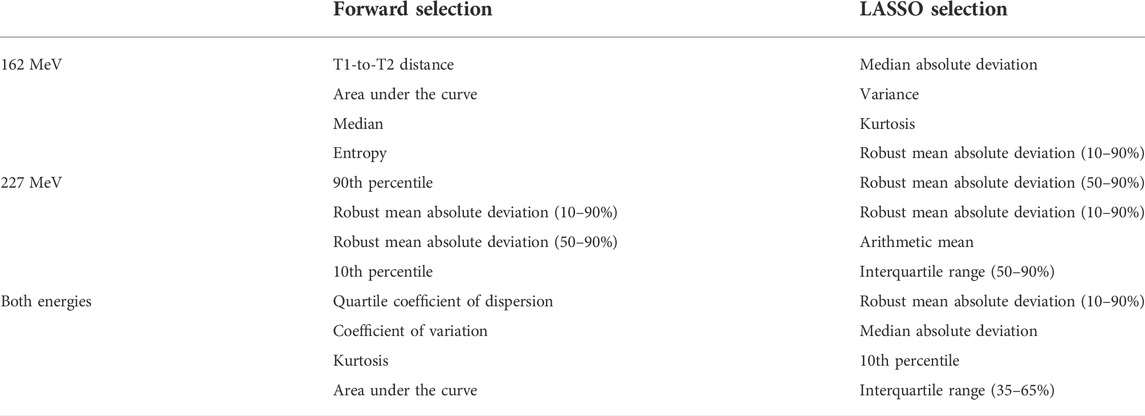
TABLE 1. The first four selected parameters for both selection methods. At four parameters, most models were close to reaching their maximum predictive power.

Correlation coefficients within the parameter assortment close to zero were found, confirming that the parameter assortment contained sufficiently independent distribution features (cf. Supplementary Figures 12–14). The parameters exhibited strong differences in their predictive value for the cavity thickness, as displayed exemplarily for 227 MeV in Figure 4 and expressed by variations in the p-value of univariate linear regression (see Supplementary Figures 15, 16).

FIGURE 4

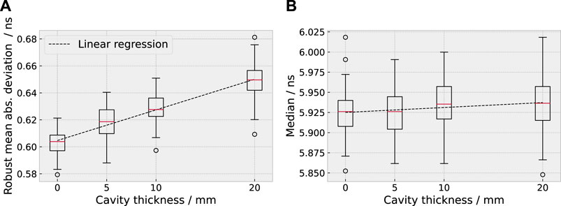
FIGURE 4. Example for a highly predictive parameter, the robust mean absolute deviation [10–90%, (A)], and a weakly predictive parameter, the median (B), for 227 MeV. The distribution of the two parameters is shown as box plot in dependence of the range deviation introduced by the cavity.

3.2 Multivariate models improve proton range prediction for static beams

In comparison to the previously used univariate models based on the mean and the standard deviation [6], the new multivariate models showed a strongly improved coefficient of determination and root mean squared error. For the energy-overarching model, R² was improved from below 0.1 to more than 0.6 by the new models and the RMSE decreased from more than 7 mm to below 5 mm (35% reduction). For the energy-specific models, R² was improved from below 0.5 to more than 0.7 and the RMSE decreased from more than 5 mm to below 4 mm (30% reduction). The two feature selection methods reached a similar coefficient of determination (agreeing within 0.1).

The predictive power either saturated or decreased after a certain amount of parameters on the validation dataset, indicating that not all selected parameters were necessary to predict the range shift (see Figure 5). Most models approached their maximum predictive power at around 3–4 parameters (except for the forward selection at 162 MeV). For the univariate models, the coefficient of determination of the energy-overarching models was strongly reduced in comparison to the energy-specific models, underlining the need for multivariate models to account for the energy-specific distribution variation.

FIGURE 5

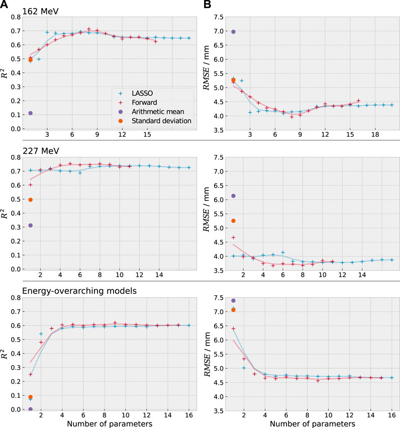
FIGURE 5. Coefficient of determination R² (A) and root mean square error RMSE (B) between predicted and actual cavity thickness for the previously used methods (violet, orange) and the newly developed statistical models (red, blue). The single data points of the new models are underlayed with a smoothed line of the same colour to improve visibility. The newly developed models exhibit a clear improvement in predictive power.

The predictive power of the energy-specific models (R² ≈ 0.75) was higher than for the energy-overarching models (R² ≈ 0.6) due to the energy-specific variability of the timing distributions. This implies that energy-specific models will be favourable in future applications.

The coefficient of determination for the training and validation dataset of the static beam experiment is depicted for both selection methods in Supplementary Section S4. The difference in the coefficient of determination between the training and validation datasets was small (below 0.1), suggesting that overfitting was avoided. Both the multivariate model of the arithmetic mean and the standard deviation and the mean of the random choice models exhibited a lower predictive power than the models defined by the first three parameters selected by forward and LASSO selection. The RMSE decreased by 0.5–1.4 mm, i.e., 10 % to 30%. This confirmed that the automated feature selection from the feature assortment provided an improvement in prediction accuracy.

3.3 Multivariate models identify cavities for scanned proton beams

As most models had approached their maximum predictive power at four parameters in the static beam experiment, the first four parameters selected by both the LASSO and forward selection methods were used to predict the proton range for the scanned field. The influence of the cavity insert on the reconstructed proton range can be observed on the range difference maps, as depicted in Figure 6 and in Supplementary Section S6.

FIGURE 6

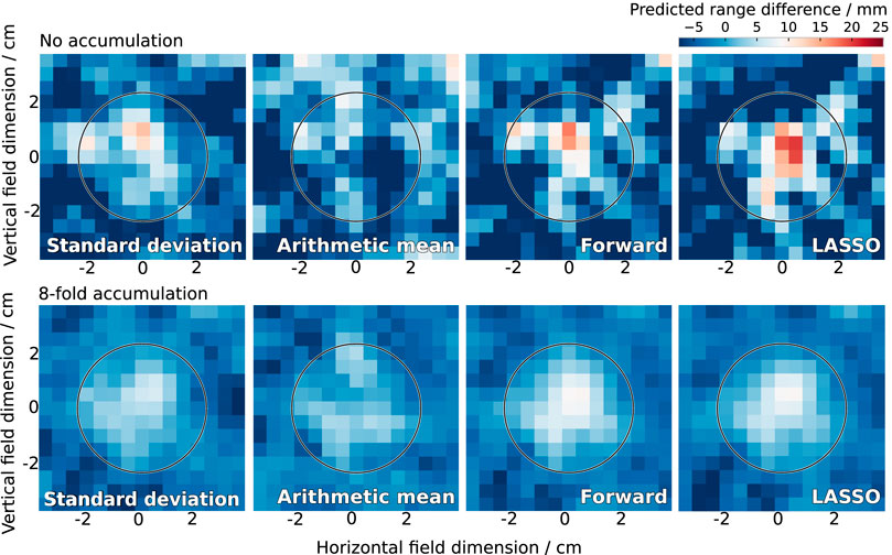
FIGURE 6. Range difference in the scanned treatment field of 227 MeV as reconstructed by the previously used methods (standard deviation, arithmetic mean) and the newly developed statistical models (forward and LASSO selection). The actual cavity thickness was 10 mm inside the circle. The colormap diverges from this actual cavity thickness in white to lower values in blue and higher values in red. The cavity was clearly detected by the new models.

At 227 MeV, the new models clearly detected all introduced range deviations, the only exception being the smallest tested cavity thickness (5 mm) without accumulation (Figure 6 and Supplementary Figures 17, 18). Without accumulation, the new models exhibited a tendency of overestimating the actual cavity thickness, whereas the previously used models showed a tendency of underestimation. With eight-fold accumulation, the agreement between actual and predicted cavity thickness was high for the new models, whereas the old models underestimated the cavity thickness. A similar behaviour was observed at the lower proton energy (162 MeV) for the model based on forward selection (Supplementary Figures 19–21).

The RMSE between actual and predicted cavity thickness for the central spots is given in Table 2. The models based on forward selection outperformed all other models, except for the case of 227 MeV without accumulation. Here, the standard deviation and the forward model performed comparably well.

TABLE 2

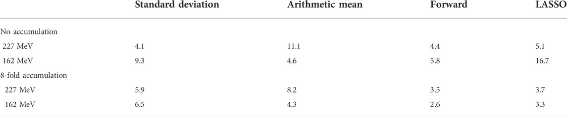
TABLE 2. RMSE between actual and predicted range deviation of the central spots in the scanned treatment field for the different parameter selection methods in mm.

Noticeably, the model defined by the LASSO selection exhibited strong fluctuations at 162 MeV when applied without accumulation, leading to an inaccurate range reconstruction (Supplementary Figures 19–21, right). The parameters selected by LASSO were strongly intercorrelated, as compared to those defined by forward selection. Therefore, the number of parameters n included in the LASSO model was successively reduced, revealing that the cavity detectability was especially reduced by the inclusion of the third parameter, i.e., the kurtosis (see Supplementary Figure S22). When limiting the model to two parameters, the performance of the LASSO model was comparable to that of the forward selection model. The inclusion of highly correlated parameters in a linear regression model can cause instability in its predictions, especially in a validation setting that differs from the training data, where extrapolation may be required. This may be the case for the model application on data of the scanning experiment. This implies that the model based on the parameters selected by forward selection was more transferable to the scanned treatment field than for those selected by LASSO at this proton beam energy.

Due to the lateral spot extension of 0.5–1.5 cm (full width at half maximum [15]), relevant range mixing occurred around the edges of the cavity for both energies, which is clearly visible in the reconstructed range maps. This points to a detectability threshold in the lateral size of the cavity.

4 Discussion

The aim of this study was to develop a range reconstruction method for prompt gamma-ray timing distributions which outperforms the methods used so far. This aim was achieved by applying forward and LASSO variable selection on a standardised histogram feature assortment and successive multivariate regression. The newly developed models showed a strongly improved predictive power (R² > 0.7) compared to the previously used models (R² < 0.5), decreased the mean prediction error by more than 1.5 mm (35%), and enabled the identification of introduced air cavities in a scanned treatment field.

It was found that one single parameter is hardly enough to reconstruct the proton range from the timing distributions. Instead, a set of approximately four parameters proved beneficial to represent the complex changes in the distribution shape. The most prognostic distribution features were found to be different measures of the distribution width, as a longer proton range corresponds to a higher probability for longer times of flight. The position of the timing peak, as represented by the arithmetic mean used in previous work, was found to be less predictive. This was most likely due to the sensitivity of the mean to outliers and remaining uncertainties in the phase shift correction. The second parameter used in previous work, the standard deviation, was found to perform better than the arithmetic mean, but still worse than the newly developed models. Especially for the higher proton energy, the introduced cavity mostly affected the second half of the timing distribution for the given phantom geometry, and this behaviour is represented better by parameters referring only to the data of the higher percentiles.

The forward and LASSO selection methods work with different optimisation criteria. Due to the broad and varied parameter assortment, the problem of finding accurate range predictors may have multiple similar solutions. Therefore, both methods did not select the same parameters but both solutions provided an improved accuracy relative to the previously used model.

Due to variations in the initial timing distributions, models trained specifically for one proton energy showed a stronger predictive power than the energy-overarching models. In clinical practice, it is possible to use energy-specific models, since the proton energy of each spot is known from the treatment plan and the machine log files. Therefore, the use of energy-specific models appears favourable for clinical application.

The main limitation of this study was the confinement of the experimental data to two irradiation scenarios (static beam and scanned layer), two proton beam energies and a simplified phantom. In this study, the phantom geometry was the same for both the training and the validation dataset. In clinical application, different anatomical changes may lead to the similar changes in the timing distributions, which may reduce the accuracy of the model prediction. The transferability of the presented method to other beam energies, full treatment plans, more anthropomorphic phantom geometries, and finally clinical patients needs to be assessed in follow-up studies. This work showed that the developed models were transferable to a scanned treatment field after being trained only on a dataset with a static beam and a different number of protons per spot. Therefore, the translation of the method to these scenarios and the development of a patient-independent model appear feasible. However, a model trained and validated on more realistic and more varied data than the static beam experiment used in this work will be necessary for clinical translation. It is likely that such a model will depend on different parameters than those selected for the simplified phantom used in this study.

For this, a large dataset covering the majority of expectable anatomical variations is required. Aside from experimental measurements, Monte Carlo based particle transport simulations may be a valuable tool to generate such a training dataset. These simulations could furthermore enable the calculation of ground-truth timing spectra for complex geometries, taking into account different material compositions and range mixing. Thus, deviations from the planned dose distribution can be detected and interpreted in more detail. However, the accuracy of simulations will be subject to systematic uncertainties in the implemented physical models, which may reduce the range prediction accuracy. The development and validation of such a simulation model is therefore of high importance and subject to future studies. As an alternative, semi-empirical analytical models of the timing distributions may prove useful. However, given the limited number of detected events per spot, it is expected to be difficult to accurately represent the various distribution shape changes, which depend on both the beam and the target properties.

The two most advanced alternative range verification systems, prompt gamma-ray imaging and spectroscopy, have been reported to currently reach a spot-wise shift detection accuracy below 2 mm [16, 17], whereas the accuracy of PGT found in this work with the presented method was still approximately 4 mm (RMSE without spot accumulation, 5 × 10³ processed events). However, these numbers are not immediately comparable since different metrics acquired under different conditions were reported and direct comparative studies are lacking so far. Both alternative methods rely on a heavy and voluminous collimator, which may limit the applicable beam angles and pose challenges for system integration [15]. On the other hand, the limited system throughput, which results in low counting statistics, is the main limiting factor for PGT. However, this limitation can easily be overcome by adding more detector units or segmented detectors [15] or optimising the electronic throuhgput [18]. Further studies will be necessary to conclusively evaluate the potential areas of application of the different systems. Possibly, a combination of multiple systems may be used, or the system choice may be entity-specific.

To further improve the range reconstruction method presented in this work, more advanced machine learning techniques than linear regression, such as support vector machines and random forests [19], may prove useful. Furthermore, the counting statistics may be improved by extending the applied energy window to cover a broader range of prompt gamma-ray energies. In addition, a promising approach is the extension of this method to two-dimensional distributions h(t_i, e_j), including the measured energy deposition e_j of the prompt gamma rays in addition to their relative detection time t_i [15]. These approaches are subject to future studies.

An important asset of the method presented in this work is that it is agnostic to the physical processes involved and the type of input data. This renders the method transferable to any system relying on a reconstruction of the proton range from one-dimensional distributions, such as the spatial (prompt gamma-ray imaging) or the energy distribution (prompt gamma-ray spectroscopy) of the prompt gamma-rays. Thus, this work can trigger future investigations to improve the prognostic value of different treatment verification systems, ultimately lowering the current limit of particle range verification accuracy.

In conclusion, this study shows that elaborate statistical modelling is a valuable tool to enhance particle treatment verification and increases its potential for routine clinical application.

Data availability statement

The original contributions presented in the study are included in the article/Supplementary Materials, further inquiries can be directed to the corresponding authors

Author contributions

SMS, TK and SL were responsible for the conception and design of the work. Data analysis was performed by JW and SMS. All authours contributed to data interpretation. SMS drafted the article. TK and SL critically revised the article. All authours approved of the final version to be published.

Acknowledgments

The authors thank Joseph Turko (Helmholtz-Zentrum Dresden—Rossendorf, Dresden, Germany) for linguistic proofreading of the manuscript.

Conflict of interest

The authors declare that the research was conducted in the absence of any commercial or financial relationships that could be construed as a potential conflict of interest.

Publisher’s note

All claims expressed in this article are solely those of the authors and do not necessarily represent those of their affiliated organizations, or those of the publisher, the editors and the reviewers. Any product that may be evaluated in this article, or claim that may be made by its manufacturer, is not guaranteed or endorsed by the publisher.

Supplementary material

The Supplementary Material for this article can be found online at: https://www.frontiersin.org/articles/10.3389/fphy.2022.932950/full#supplementary-material

Footnotes

¹Scionix Holland B.V., Regulierenring 5, 3981 LA Bunnik, Netherlands

²Hamamatsu Photonics K.K., 325–6, Sunayama-cho, Naka-ku, Hamamatsu City, Shizuoka Pref., 430–8587, Japan

³Target Systemelektronik GmbH & Co. KG, Heinz-Fangman-Straße 4, 42287 Wuppertal, Germany

⁴This number of protons corresponds approximately to that of 8 strongly weighted clinical pencil beam scanning spots (1.25 × 10⁸ protons per spot) or the combined signal of 8 prompt-gamma ray detectors for one strongly weighted clinical pencil beam scanning spot. The currently envisioned PGT system consists of 8 detectors attached in a circle around the treatment head [6].

References

1. Jäkel O. Medical physics aspects of particle therapy. Radiat Prot Dosimetry (2009) 137:156–66. doi:10.1093/rpd/ncp192

PubMed Abstract | CrossRef Full Text | Google Scholar

2. Lomax AJ. Intensity modulated proton therapy and its sensitivity to treatment uncertainties 2: The potential effects of inter-fraction and inter-field motions. Phys Med Biol (2008) 53:1043–56. doi:10.1088/0031-9155/53/4/015

PubMed Abstract | CrossRef Full Text | Google Scholar

3. Engelsman M, Bert C. Precision and uncertainties in proton therapy for moving targets. In: H Paganetti, editor. Proton therapy physics. Florida: CRC Press, Taylor & Francis Group (2011). p. 435–60.

CrossRef Full Text | Google Scholar

4. Pausch G, Müller C, Berthold J, Enghardt W, Küchler M, Römer K, et al. Effect of strong load variations on gain and timing of CeBr₃ scintillation detectors used for range monitoring in proton radiotherapy. In: IEEE Nuclear Science Symposium and Medical Imaging Conference; 10-17 Nov 2018; Sydney, Australia (2018).

Google Scholar

5. Golnik C, Hueso-González F, Müller A, Dendooven P, Enghardt W, Fiedler F, et al. Range assessment in particle therapy based on prompt γ-ray timing measurements. Phys Med Biol (2014) 59:5399–422. doi:10.1088/0031-9155/59/18/5399

PubMed Abstract | CrossRef Full Text | Google Scholar

6. Werner T, Berthold J, Hueso-González F, Kögler T, Petzoldt J, Römer K, et al. Processing of prompt gamma-ray timing data for proton range measurements at a clinical beam delivery. Phys Med Biol (2019) 64:105023. doi:10.1088/1361-6560/ab176d

PubMed Abstract | CrossRef Full Text | Google Scholar

7. Jacquet M, Marcatili S, Gallin-Martel ML, Bouly JL, Boursier Y, Dauvergne D, et al. A time-of-flight-based reconstruction for real-time prompt-gamma imaging in proton therapy. Phys Med Biol (2021) 66:135003. doi:10.1088/1361-6560/ac03ca

CrossRef Full Text | Google Scholar

8. Pennazio F, Ferrero V, D’Onghia G, Garbolino S, Fiorina E, Villarreal OAM, et al. Proton therapy monitoring: Spatiotemporal emission reconstruction with prompt gamma timing and implementation with PET detectors. Phys Med Biol (2022) 67:065005. doi:10.1088/1361-6560/ac5765

CrossRef Full Text | Google Scholar

9. Werner T, Berthold J, Enghardt W, Hueso-González F, Kögler T, Petzoldt J, et al. Range verification in proton therapy by prompt gamma-ray timing (PGT): Steps towards clinical implementation. In: 2017 IEEE Nuclear Science Symposium and Medical Imaging Conference; 21-28 October 2017; Atlanta, GA, USA. NSS/MIC (2017). p. 1–5. doi:10.1109/NSSMIC.2017.8532807

CrossRef Full Text | Google Scholar

10. Zwanenburg A, Leger S, Vallieres M, Löck S. Image biomarker standardisation initiative reference manual. arXiv (2019). doi:10.48550/arXiv.1612.07003

CrossRef Full Text

11. Marcatili S, Collot J, Curtoni S, Dauvergne D, Hostachy JY, Koumeir C, et al. Ultra-fast prompt gamma detection in single proton counting regime for range monitoring in particle therapy. Phys Med Biol (2020) 65:245033. doi:10.1088/1361-6560/ab7a6c

PubMed Abstract | CrossRef Full Text | Google Scholar

12. Draper NR, Smith H. Applied regression analysis. New York: John Wiley & Sons (1966).

Google Scholar

13. Kuhn M, Johnson K. Applied predictive modeling. New York: Springer (2013). doi:10.1007/978-1-4614-6849-3

CrossRef Full Text | Google Scholar

14. Van Rossum G, Drake FL. Python 3 reference manual. Scotts Valley, CA: CreateSpace (2009).

Google Scholar

15. Pausch G, Berthold J, Enghardt W, Römer K, Straessner A, Wagner A, et al. Detection systems for range monitoring in proton therapy: Needs and challenges. Nucl Instr Methods Phys Res Section A (2020) 954:161227. doi:10.1016/j.nima.2018.09.062

CrossRef Full Text | Google Scholar

16. Nenoff L, Priegnitz M, Janssens G, Petzoldt J, Wohlfahrt P, Trezza A, et al. Sensitivity of a prompt-gamma slit-camera to detect range shifts for proton treatment verification. Radiother Oncol (2017) 60:P534–40. doi:10.1016/j.radonc.2017.10.013

CrossRef Full Text | Google Scholar

17. Hueso-González F, Rabe M, Ruggieri TA, Bortfeld T, Verburg JM. A full-scale clinical prototype for proton range verification using prompt gamma-ray spectroscopy. Phys Med Biol (2018) 63:185019. doi:10.1088/1361-6560/aad513

PubMed Abstract | CrossRef Full Text | Google Scholar

18. Hueso-González F, Casaña Copado JV, Fernández Prieto A, Gallas Torreira A, Lemos Cid E, Ros García A, et al. A dead-time-free data acquisition system for prompt gamma-ray measurements during proton therapy treatments. Nucl Instr Methods Phys Res Section A (2022) 1033:166701. doi:10.1016/j.nima.2022.166701

CrossRef Full Text | Google Scholar

19. Hastie T, Tibshirani R, Friedman J. The elements of statistical learning: Data mining, inference, and prediction. New York, USA: Springer (2016).

Google Scholar