 Nara Guisoni
 Luis Diambra
94% of researchers rate our articles as excellent or good
Learn more about the work of our research integrity team to safeguard the quality of each article we publish.
Find out more
ORIGINAL RESEARCH article
Front. Phys., 22 July 2022
Sec. Biophysics
Volume 10 - 2022 | https://doi.org/10.3389/fphy.2022.927152
This article is part of the Research TopicPattern Formation in BiologyView all 13 articles
One of the most surprising mechanisms to explain the symmetry breaking phenomenon linked to pattern formation is known as Turing instabilities. These patterns are self-organising spatial structures resulting from the interaction of at least two diffusive species in specific conditions. The ideas of Turing have been used extensively in the specialised literature both to explain developmental patterns, as well as synthetic biology design. In the present work we study a previously proposed morphogenetic synthetic circuit consisting of two genes controlled by the same regulatory system. The spatial homogeneous version of this simple model presents a rich phase diagram, since it has a saddle-node bifurcation, spirals and limit cycle. Linear stability analysis and numerical simulations of the complete model allow us to determine the conditions for the development of Turing patterns, as well as transient patterns. We found that the parameter region where Turing patterns are found is much smaller than the region where transient patterns occur. We observed that the temporal evolution towards Turing patterns can present one or two different length scales, depending on the initial conditions. Further, we found a parameter region where the persistence time of the transient patterns depends on the distance between the parameters values on which the system is operating and the boundary of Turing patterns. This persistence time has a singularity at a critical distance that gives place to metastable patterns. To the best of our knowledge, transient and metastable patterns associated with Turing instabilities have not been previously reported in morphogenetic models.
Pattern formation in morphogenetic system is one of the central problems in developmental biology. One of the best-known mechanism of autonomous pattern formation is the Turing instability. This symmetry breaking mechanism was introduced in 1952 by Alan Turing in the context of models for morphogenesis [1]. The basic idea is that Turing instability arises from the coupling between diffusion and reaction which can destabilize spatially homogenous equilibrium and lead to the formation of patterns. The minimum biological system able to present Turing instabilities consists in only two interacting diffusible components: an activator with a slow diffusion rate and an inhibitor with a fast diffusion rate [2].
There is a large body of literature focused on the mechanism proposed by Turing to explain the patterns of self-organization during the animal development [3–11]. However, the identification of the molecular agents driving Turing patterns remains an unsolved issue in most cases.
Thanks to recent progress in synthetic genetic circuit engineering, several researchers have embarked on the implementation of Turing ideas on cell culture [12–17]. To engineer such biological systems, one needs to know the mandatory properties and genetic circuit that support the biological patterning process. It is well known that two key factors underlying the Turing model are the differential diffusion between activator and inhibitor, and also the non-linearity in the reactive terms. In addition, it has been shown that the latter can be as important as the differential diffusion [18, 19]. In this sense, a Turing model has been proposed where the activator and inhibitor are under the control of the same promoter, a simplification that can be exploited in the design of synthetic morphogenetic circuits. This biological simplification allows a mathematical analysis which has highlighted the role of cooperative regulation as source of non-linearity [18]. However, beyond this contribution, the single-promoter model has not been explored to its full potential in either theoretical or experimental studies. In this paper we present a deep theoretical analysis of this simple model and report that it has a rich phase diagram that include: saddle-node, limit cycles and Turing patterns. We also observe transient patterns, driven by Turing instability, which hereafter will be referred to as transient Turing patterns. Previous reports about transient Turing patterns have been done in the context of closed systems, when chemical species are being consumed [20–22] and for noise-driven stochastic patterns in a multicellular cyanobacterial organism [23]. Moreover, out of the reaction-diffusion context, transient Turing patterns have been reported in a neural field model of working memory [24]. Except for the last case, the reaction-diffusion systems associated with transient Turing patterns are composed by several species, which posses the additional challenge to derive analytical predictions or to associate a phase diagram to study them. On the other hand, the present model can be associated with biological systems [25, 26] and the analysis of the associated reaction-diffusion equations are feasible for some values of the Hill exponent of regulatory function. The present results show that in this model the transient patterns are due to the presence of a saddle node which have associated spatial modes with no-null amplification rate. Patterns initiated around this steady state can experiment a transition to Turing pattern associated with a stable steady state, or disappear. The existence of transient patterns brings with it the question of their persistence. This question is especially important given that in the biological context Turing patterns are associated with spatial distributions of molecules that induce morphogenetic processes whose time scales must be finely orchestrated. Interestingly, we observe that the persistence time of the transient patterns suffers a critical transition when parameters values approaches at a critical distance of the boundary that separate Turing stable patterns. This critical distance defines a region for metastable patterns, where the spatial pattern remains stable over large time scales while no disturbances operate. Metastable transient patterns have been previously reported in the context of 1D reaction-diffusion systems [27, 28]. To the best of our knowledge, metastable Turing patterns are a novel feature as far as morphogenetic models are concerned, because are related to unstable nodes, which have not been considered in previous studies on Turing instability.
The minimum biological system able to present Turing instabilities consists of two interacting diffusible proteins, named morphogens. In the case of the model considered here, the self-activating morphogen A also activates the morphogen H, which in turn inhibits both morphogens (see the sketch in Figure 1A). The activator and the inhibitor morphogens are coupled through the regulatory functions associated with the genes that encode them. The regulatory functions describe mathematically how the protein synthesis rate depends on the concentration of activators and inhibitors. A morphogenetic model was recently introduced which considers that both morphogens are regulated by the same promoter [18]. That means that regulatory functions that control the synthesis rate of both morphogens will be the same. Thus, in this case, the temporal evolution of the system is described by a couple of reaction-diffusion equations of the form.
Where a (x, t) and h (x, t) denote the concentration of the activator A and the inhibitor H, respectively, as a function of spatial position and time. The last term on the right hand side of each equation describes the degradation process and was assumed to be linear. The function f corresponds to the regulatory function that controls the expression of both activator and inhibitor. As in the previous study [18], we consider a sigmoidal regulatory function where activator and inhibitor compete for the same regulatory site in the form:
where nH is the Hill exponent that describes the steepness of the sigmoidal function (considered equal for both activator and inhibitor), while ka and kh are related to the effective dissociation constant for the activator and inhibitor, respectively. However, non-competitive regulatory function can also be used [29, 30]. At this point it is convenient to introduce dimensionless variables for time
To simplify the notation we introduced the abbreviations d = Da/Dh, μ = μh/μa,
Where.
Next, we carried out a detailed mathematical analysis of local stability of this dimensionless model for the case without diffusion. After that, we presented the Turing-instability conditions. From now on we will write new variables without the hat in order to simplify the notation. The Hill exponent on the regulatory function f is usually associated with the number of regulatory sites in the promoter, but as a consequence of the finite free energy involved in the interaction between regulators molecules [31, 32], the exponent is not an integer number. Despite that, hereafter we set nH = 2 for mathematical convenience since it allows the derivation of analytical expressions which will help to obtain the results on the next Section.
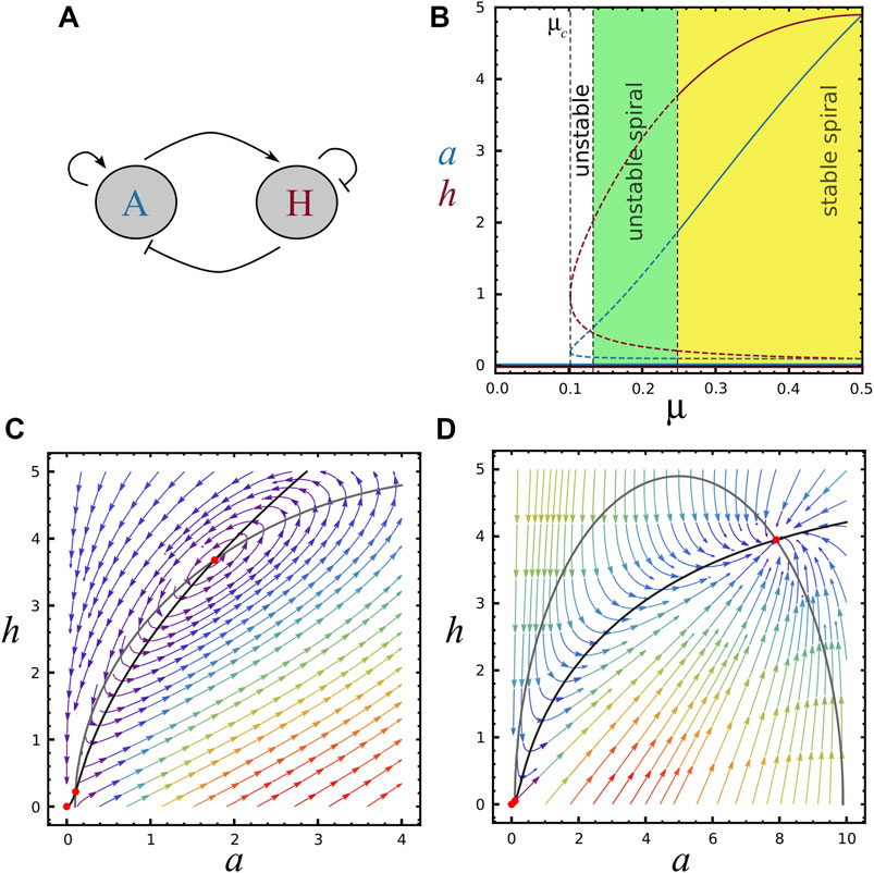
FIGURE 1. Bifurcation diagram and nullclines, (A) Schematic representation of the two-component system, A is the activator morphogene (activates both reactants), H is the inhibitor morphogene (inhibits both reactants). (B) Bifurcation diagram showing the behavior of concentrations a (blue) and h (red) as a function of μ, with ra =10 and rh =5. The trivial fixed point S0=(0,0) is present for all μ values. The saddle-node bifurcation at μ = μc ≈0.10 marks the emergence of two new fixed points (S1 and S2). Continuous and dashed curves represent respectively regions of stable and unstable steady state solutions. Black vertical dashed lines refer to μc and the stability of steady-state S2, indicating regions of unstable node (white area, where TrA <0, det A >0 and Δ >0), unstable spiral (green area, where TrA <0, det A >0 and Δ <0) and stable spiral (yellow area, where TrA >0, det A >0 and Δ <0). For μ = μ2 the system displays a limit cycle (TrA =0 and det A >0). For visualisation in the phase diagram, see horizontal line in Supplementary Figure S1B. (C) Black and grey curves represent F and G functions (nullclines) for the parameters value (μ, ra, rh)=(0.24,10,5) (S2 is an unstable spiral). (D) Nullclines for the parameters value (μ, ra, rh)=(1,10,5) (S2 is a stable node). Red points represent fixed points.
In order to determine the general conditions for diffusion-driven instabilities, it is necessary to study the temporal evolution of the diffusion-less system:
The homogeneous steady states S = (ass, hss) system of (Eqs. 8, 9) are the positive solutions of equations F (ass, hss) = 0 and G (ass, hss) = 0. The system can present up to three fixed points: the trivial solution S0 = (0, 0), and two non-trivial solutions, identified as S1 = (a1, h1) and S2 = (a2, h2) with.
The non-trivial steady-states, S1 and S2, are real in a parameter region defined by
Hence,
For μ > μc the three steady-states are real, while for μ < μc only the trivial one is found. For μ = μc the two non-trivial solutions merge together (see Figure 1B). Similarly, we can obtain analytical expressions for critical values of ra and rh as a function of the remaining parameters.
In Figure 1B it is possible to appreciate the activator and inhibitor concentrations as a function of μ for the three steady states, when ra and rh are kept as constants. Note that μ = μc is a saddle-node bifurcation and the non-trivial stead-states S1 and S2 are present only for μ > μc. Similarly, Supplementary Figure S1A shows a and h as a function of rh keeping constants μ and ra. Supplementary Figure S1B depicts a stability phase diagram for S2 in the plane μ-rh with ra = 10, where the different regions of stability are indicated by colors. Horizontal dashed line shows the section of the parameter region explored in Figure 1B (ra = 10 and rh = 5), with dots indicating the dashed lines of Figure 1B. Vertical dashed line shows the section of the parameter region explored in Supplementary Figure S1A.
Typical phase planes can be seen in Figures 1C,D, for different values of μ. Note that increasing μ brings S0 and S1 closer together, as it can also be seen in Figure 1B.
Linearising the system about the steady-states S = (ass, hss) it is possible to determine the stability of each state S. Therefore, we define
For the case of |v| small, it is possible to approximate Eqs. 8 and 9 as
where A is the Jacobian matrix, with
with
The trivial steady-state S0 is always a stable node, whereas S1 is an unstable saddle-point for the parameter region delimited by the inequality (Eq. 12). S2 has a more intricate behaviour, as it is discussed below.
The stability of S2 depends on the values of ra, rh and μ, as shown in Figure 2A. As it can be seen, the region where S2 is stable becomes smaller as the inhibitor production rate rh increases. On the other hand, this region rises with the activator production rate ra and the relative degradation rate μ. We observe that a and h concentrations in S2 can present oscillations, which can be stable or unstable (see Figure 2B). Interestingly, in the region of unstable spirals (where TrA > 0 and Δ < 0), oscillations drive the system to the trivial steady-state S0 (see Figure 2C and the phase-plane of Figure 1C). Otherwise, when TrA < 0 (with Δ < 0) the stable spirals around S2 are damped until the system reaches the stable steady-state (see Supplementary Figure S1C). On the boundary of unstable and stable spirals, when Reλ = 0 and Imλ ≠ 0 (TrA = 0 and det A > 0), a stable limit circle is found, as shown in Supplementary Figure S1D. The rich behaviour of the system around S2 can also be seen in the μ-rh phase diagram of Supplementary Figure S1B: four regions indicate when S2 is an unstable node, unstable spiral, stable spiral or stable node. Besides, the saddle-node bifurcation line and the limit-circle line are shown.
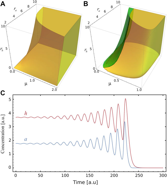
FIGURE 2. Stability and instability of the fixed point S2. (A) Yellow volume delimits, in the parameters space (μ, ra, rh), the region where the steady state S2 is stable. (B) The green region corresponds to the values of the parameters where the system develops a spiral source behaviour in the steady state S2 (see panel C), while in the yellow region there is a spiral sink behaviour at S2. Only at the interface of these two regions does the system exhibit a limit cycle. (C) Example illustrating of unstable oscillatory behaviour for a and h, as function of time, for (μ, ra, rh)=(0.24,10,5), the amplitudes increase until they reach the stable trivial fixed point S0.
In Figure 1B the stability of S2 for increasing μ is presented: it changes from an unstable node to unstable and stable oscillations. In the phase-plane of Figure 1C, S2 is an unstable spiral while for Figure 1D it is a stable node. The stability of S2 as a function of rh is shown in Supplementary Figure S1A. In this case, greater values of rh lead the system towards instability. The points μ = μc and rh = rhc shown respectively in Figure 1B and Supplementary Figure S1A, where S1 = S2, are saddle points.
As it was mentioned in the previous section, the fixed point S2 is stable in a region of the parameter space. The addition of diffusive terms to the system of (Eqs. 8, 9) can destabilise the spatially homogeneous equilibrium and lead to the formation of patterns, known as Turing patterns. To obtain the mathematical conditions for Turing instability let us consider a one-dimensional version of Eq. 15, that includes the diffusive process,
and the boundary conditions. We are interested in the zero-flux boundary condition, i.e., that morphogens cannot diffuse beyond the boundaries [0,L]. This implies that the wave number k of solutions of Eq. 18 takes discrete values kn = nπ/L, with n = 0, 1, 2, …. As usual, the steady solution S is perturbed with
The perturbation
Therefore, for the stable homogeneous state to become unstable upon perturbation δn it is required that Re(ω) > 0. This is fulfilled if any of the conditions below are satisfied
As (Eq. 21) is never true for a stable fixed point, the only necessary condition is (Eq. 22). Taking into account that det A > 0 on stable fixed point, condition (Eq. 22) implies in
The condition for a non-trivial solution Eq. 20 leads to the relation of the eigenvalues as function of the wave number k, knows as dispersion relation
where α(k) and β(k) are functions of k2 and given by
where the partial derivatives of F and G are evaluated at the steady-state S under consideration. In the following we will consider only the dispersion relation ω+ because ω− is negative in the parameter region of interest.
Furthermore, we are looking for positive k2 such that β(k) < 0 for some nonzero k. Thus it is necessary that the minimum of β be negative. By differentiating with respect to k2 we obtain that the minimum of β is at
Thus, the necessary and sufficient conditions for Turing instability can be summarised by the conditions for the existence of a stable homogeneous state in the absence of diffusion (Eq. 17), and conditions (Eq. 23) and (Eq. 27). These four conditions determine that the system will develop Turing patterns when a stable fixed point is disturbed by a perturbation with a certain wave number.
Figure 3A depicts the region of the parameter space spanned by parameters μ, ra and rh where the reaction-diffusion system of (Eqs. 8, 9) satisfies the conditions for Turing instabilities for d = 0.01. However, we observe that some perturbations can also propagate even when the fixed point in question is unstable, given rise in this case to transient patterns, or transitions between spatial patterns with different wave numbers. To analyse this aspect lets us remark that the temporal evolution of a spatial perturbation is dominated by the value of the wave number associated with the largest amplification rate, i.e., k value which maximises
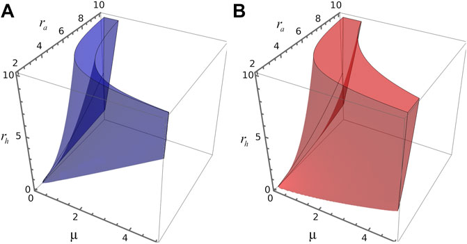
FIGURE 3. 3D parameters space. (A) Blue volume delimits, in the space spanned by parameters (μ, ra, rh), the region where the four Turing conditions are verified for steady state S2. (B) Red volume delimits, in the space spanned by parameters (μ, ra, rh), the region where k2>0 and ω >0 for the steady state S1.
To illustrate some features of stable and transient Turing patterns, we perform 1D simulations of the reaction-diffusion equations at different values of the parameters μ, ra and rh. In Figure 4A we superpose Figures 3A,B on the plane spanned by parameters μ and rh for ra = 6. In this way, we identify the region where stable Turing patterns are found (overlap between R1 and R2, light blue); and the region where only transient patterns are observed (R2, red). Black points in the plane correspond to parameter values used in different numerical simulations. Figure 4B depicts the Turing patterns developed by the activator, for parameters (μ, ra, rh) = (1, 6, 10). In both simulations the spatial perturbation is the same, ∝ exp [ − (x − 40)2/0.25], however the simulations differ in the initial spatial distribution to be perturbed. The top panel of Figure 4B corresponds to a perturbation of homogeneous distribution associated with the fixed point S1 (saddle node), while the bottom panel corresponds to a perturbation of homogeneous distribution associated with the stable fixed point S2. In the first case the system develops quickly a central pattern, with small wave number. Over time, the ridges split in two, increasing the wave number of the pattern. These splits evidence the transition to a stable Turing pattern with the same wave number as that observed in the bottom panel. We also see in Figure 4B that the amplification rate of the perturbation of S2 is lower than in the case where S1 is perturbed.
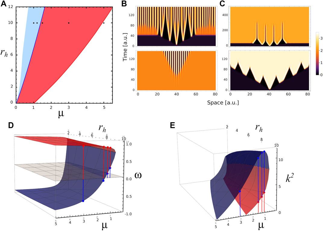
FIGURE 4. Different spatial scales. (A) 2D phase diagram shows the parameters region where the system presents stable Turing patterns (blue area) and unstable or transient Turing patterns (red area) for ra=6.0. Black dots correspond to different triplet of parameters values (μ, ra, rh) where numerical simulation were performed: P1=(1.0,6,10), P2=(1.2,6,10) in the Turing pattern region, P3=(1.5,6,10), P4=(3.0,6,10) in the transient Turing pattern region, and P5=(5.0,6,10) in the region for uniform distributions. (B) 1-D numerical simulations showing the temporal evolution of activator concentration distribution a for parameters value P2 with two different initial conditions. Top (bottom) panel corresponds to the temporal evolution when fixed point S1 (S2) is perturbed by a small perturbation at x =40, note the different spatial scales of patterns on the panels. The temporal evolution of a for parameters values P1, P3 and P5 are shown in Supplementary Figure S2. (C) 1-D numerical simulations showing the temporal evolution of a for parameters values P3 (top panel) and P4 (bottom panel) when the same fixed point S1 is perturbed at x = 40. (D) Red and blue surfaces correspond to ω-value as function of μ and rh associated with fixed points S1 and S2, respectively. (E) k2-values as function of μ and rh associated with S1 (red surface) and S2 (blue surface). In both panels D and E, ra =6.0, and the red and blue dots indicate ω and k2 values for P1, P2, P3 and P4 in each case.
We also perform numerical simulations in the region of transient patterns for μ = 1.5 and 3.0 (top and bottom panels of Figure 4C), when a small perturbation is applied on fixed point S1. In these cases the system makes a transition to a stable homogeneous distribution associated with state S2. These transitions occur in a spatially heterogeneous manner, as long as ω(S1) and
In an effort to further understand the transient patterns exhibited by our model, Figure 5 depicts analyses and simulations for ra = 2.5 where there is a narrow region for Turing instabilities (light blue region) and a large region for transient Turing patterns (red region). In this case, the
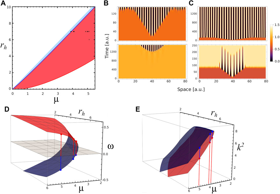
FIGURE 5. Different time scales. (A) 2D phase diagram shows the parameters region where the system presents stable Turing patterns (narrow blue area) and unstable or transient Turing patterns (blue area) for ra =2.5. Black dots correspond to different triplet of parameters values (μ, ra, rh) where numerical simulation were performed: P1=(3.9,2.5,7), in the Turing pattern region, P2=(4.1,2.5,7) and P3=(5.0,2.5,7) in the transient Turing pattern region. The crosses indicate parameters values used on Figure 6. (B) 1-D numerical simulations showing the temporal evolution of activator concentration distribution a for parameters value P1 with two different initial conditions. Top (bottom) panel corresponds to the temporal evolution when fixed point S1 (S2) is perturbed by a small perturbation at x =40, note the different timescales on the panels. (C) 1-D numerical simulations showing the temporal evolution of a for parameters values P2 (top panel) and P3 (bottom panel) when the same fixed point S1 is perturbed at x =40, note the different timescales on the panels. (D) Red and blue surfaces correspond to ω-value as function of μ and rh (ra =2.5) associated with fixed points S1 and S2, respectively. (E) k2-values as function of μ and rh associated with S1 (red surface) and S2 (blue surface). Red and blue dots indicate k2 values for P1, P2 and P3 in each case.
Regarding the pattern on Figure 5C, we hypothesise that when the parameter values approach to the boundary between regions of stable and transient Turing patterns (blue line in Figure 5A), the resulting transient patterns would be associated with larger half-lives. Let us define the persistence time of a transient pattern, τ, as the duration of the central ridge, that is before it merges with the neighbours ones; and b as the Euclidean distance from actual parameters value to the boundary between regions of stable and transient Turing patterns. Following our ansatz, we compute the persistence time τ on several transient patterns, depicted on panels A–E of Figure 6, obtained for ra = 2.5, and different values of rh and μ. Also, Figure 6F depicts the persistence time as function of the distance b. Interestingly, the plot suggests that near Turing-patterns boundary the persistence time exhibits a singularity at bc. This means that, in this region of the parameters space (ra = 2.5 and rh ≈ 7.0), a system operating with parameters value corresponding to b smaller than bc will present patterns with infinite persistence time, i.e. metastable patterns. This is the case of the top panel of Figure 5C. This could be a particular characteristic of this region, since no metastable patterns were observed in the parameter region studied in Figure 4 (ra = 6), where transient patterns were also observed.
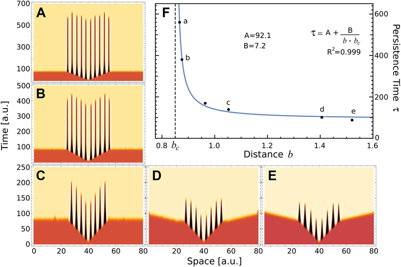
FIGURE 6. Persistence time. (A–E) These panels depict the temporal evolution of a, when the uniform distribution associated with fixed point S1 is perturbed at x =40, for different values of the parameters (μ, ra, rh)=(4.89,2.5,7) (A) (4.9, 2.5,7) (B) (5.1,2.5,7) (C) (5.5,2.5,7) (D) and (5.1,2.5,6) (E). These parameters values were indicated by crosses on 5A. (F) Raster-plot of persistence time τ and distance b for the numerical simulations (A–E) and also P3=(5.0,2.5,7) depicted in bottom panel of 5C. Blue line corresponds to the rational function A+ B/(b − bc), where the value of parameters were obtained by nonlinear fitting (A =92.1, B =7.2 and bc =0.85). Letters a-e indicated the corresponding panel.
These results suggest the existence of a new interface separating two types of transients Turing patterns associated to S1: those with finite τ and the metastable patterns. Although establishing the mechanisms that determine this interface is beyond the scope of this work, we believe that the morphogenetic model proposed by Diambra et al. could be suitable for such study. To the best of our knowledge, transient and metastable patterns arising from Turing instability mechanism have not been previously reported.
As noticed in the previous subsections, the trajectory of the system upon perturbation depends on whether the system is initially on state S1 or S2, however the final states after a transient are the same (as shown in Figure 4B, Figure 5B). We wonder if this also happens in two dimensions. And to answer this question we performed numerical simulations of Eqs. 4 and 5 in a 2D region Ω = [0, 40] × [0, 40] with periodic boundary conditions. In order to solve the equations, we discretized space and time using NDSolve routine in Mathematica 12.1, in which we take Δx = Δy = 0.01. The temporal step size used is adaptative so that the estimated error in the numerical solution is lower than 10–6. We consider the same perturbation
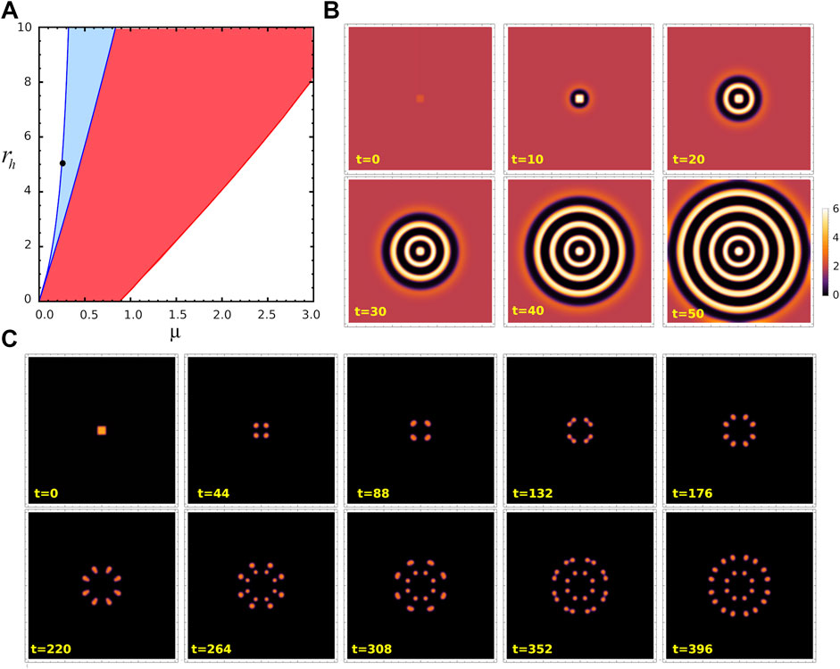
FIGURE 7. Turing patterns in 2D. (A) Parameter region where stable Turing patterns (blue) and unstable Turing patterns (red) can be found, for ra =10. Black dot corresponds to (μ, ra, rh)=(0.25,10,5)= P1, in the stable Turing pattern region. (B) Snapshots from space-temporal 2D simulations showing activator concentration pattern for parameters value P1 at different time t. These panels corresponds to the case when fixed point S2 is perturbed by a small perturbation at the centre of the field. (C) Snapshots from space-temporal 2D simulations showing a for the same parameters value, when uniform distribution associated to fixed point S1 is perturbed by the same perturbation. The region considered is 40×40 with periodic conditions. Animated Movies associated to these simulations are available as Supplementary Movies S1 and S2.
In this paper we have analysed a two-gen reaction–diffusion system that operates under only one regulatory function, as previously proposed by [18]. The non-diffusive model presents three fixed points. One of them corresponds to the trivial solution and is referred to as S0, while the other two non-trivial solutions, identified as S1 and S2, are originated in a saddle-node bifurcation. We obtain analytically that the saddle-node bifurcation defines a surface in the 3D parameter space. The trivial solution S0 is a stable node and S1 is an unstable saddle-point for all the parameter region studied. On the other hand, S2 is stable for a certain region of the parameter space and when perturbed can also present oscillations and a stable limit circle. In the region of unstable spirals of S2, oscillations drive the system to the trivial steady-state S0, while stable spirals are damped until the perturbed system reaches S2.
To derive the Turing-instability conditions, one requires an stable homogeneous steady state, like S2, to guarantee that instabilities will be solely spatially dependent. However, diffusion-driven patterns can also raise up from an unstable steady state, like S1. In fact, by linearizing the spatial version of the model around these steady states we found that both points have associated a dispersion relation where ω > 0 and k > 0, indicating the presence of a spatial patterns. We denote the parameter region where S1 has ω > 0 and k > 0 as R1. Similarly, in R2 the steady state S2 has ω > 0 and k > 0. We observe that R1 is greater than R2 and R2 is included in R1.
The final state of the system, when a small spatial perturbation is applied to S1 or S2 fixed points, depends on where the parameters value falls relative to R1 or R2. As expected, we observe that a spatial perturbation of the S2 state, for parameters values belong to R2, leads to stable Turing patterns. On the other hand, if S2 is perturbed for parameters values outside R2, no pattern will be developed. When S1 is perturbed for parameter values that are in the intersection region of R1 and R2, then a spatially heterogeneous transition to stable Turing patterns with sizes typical of the S2 state develops. In this sense we have seen examples where the initial peaks with typical size of the state S1 split. But if the values of the parameters fall outside R2 and inside R1, the system develops in the face of disturbance a transient spatial pattern whose typical size is predicted by the dispersion relation in S1. In the region of the parameter space with low ra-value, the system can present transitory patterns, as well as metastable patterns. In the former case, we observed that the persistence time of these transitory patterns is related to the distance between the value of the system parameters and the boundary between regions of stable and transient Turing patterns. We found that this dependence has a singularity which delimits a new boundary between metastable patterns and transient patterns with finite time life. However, the present analysis did not allow to determines the boundary, in the parameters space, separating metastable patterns and short transients.
Furthermore, in the synthetic patterning endeavour is critical the range of kinetic parameters, Hill coefficient and diffusion ratio between activator and inhibitor, that support Turing patterns development [18]. Consequently, alternatives to reduce the requirement for differential diffusion are always welcomed. The present results show that transient patterns can expand the parameter space for an initial breaking-symmetry. These initial patterns, although transient, could induce other gene regulatory circuits able to stabilise patterning but without breaking-symmetry ability. In this manner, transient patterns could play a role in developmental biology as breaking-symmetry triggers rather than to be responsible for the whole patterning process. We believe that the current findings open the door to further theoretical studies which can offer new insights into the nature of patterning mechanisms in developmental biology.
The original contributions presented in the study are included in the article/Supplementary Material, further inquiries can be directed to the corresponding authors.
LD conceived the paper. NG and LD developed the structure and design of the manuscript. NG and LD developed the analysis, and algorithms and wrote the manuscript. Both NG and LD revised the manuscript and approved the final version.
This research was supported by CONICET, Argentine (PIP N° 0597 and PIP N° 1748).
NG and LD are reasearchers at the CONICET (Argentine). We are thankful for Karina Mazzitello’s judicious comments on the manuscript, and Celina Guisoni’s help in preparing graphics.
The authors declare that the research was conducted in the absence of any commercial or financial relationships that could be construed as a potential conflict of interest.
All claims expressed in this article are solely those of the authors and do not necessarily represent those of their affiliated organizations, or those of the publisher, the editors and the reviewers. Any product that may be evaluated in this article, or claim that may be made by its manufacturer, is not guaranteed or endorsed by the publisher.
The Supplementary Material for this article can be found online at: https://www.frontiersin.org/articles/10.3389/fphy.2022.927152/full#supplementary-material
1. Turing AM. The chemical basis of morphogenesis. Philos Trans R Soc B (1952) 237:37. doi:10.1098/rstb.1952.0012
2. Meinhardt H, Gierer A. Applications of a theory of biological pattern formation based on lateral inhibition. J Cel Sci (1974) 15:321. doi:10.1242/jcs.15.2.321
3. Asai R, Taguchi E, Kume Y, Saito M, Kondo S. Zebrafish leopard gene as a component of the putative reaction-diffusion system. Mech Dev (1999) 89:87–92. doi:10.1016/s0925-4773(99)00211-7
4. Painter KJ, Maini PK, Othmer HG. Stripe formation in juvenile pomacanthus explained by a generalized Turing mechanism with chemotaxis. Proc Natl Acad Sci U S A (1999) 96:5549–54. doi:10.1073/pnas.96.10.5549
5. Diambra L, Costa LDF. Pattern formation in a gene network model with boundary shape dependence. Phys Rev E (2006) 73:031917. doi:10.1103/PhysRevE.73.031917
6. Yamaguchi M, Yoshimoto E, Kondo S. Pattern regulation in the stripe of zebrafish suggests an underlying dynamic and autonomous mechanism. Proc Natl Acad Sci U S A (2007) 104:4790–3. doi:10.1073/pnas.0607790104
7. Kondo S, Miura T. Reaction-diffusion model as a framework for understanding biological pattern formation. Science (2010) 329:1616–20. doi:10.1126/science.1179047
8. Salazar-Ciudad I, Jernvall J. A computational model of teeth and the developmental origins of morphological variation. Nature (2010) 464:583–6. doi:10.1038/nature08838
9. Sheth R, Marcon L, Bastida MF, Junco M, Quintana L, Dahn R, et al. Hox genes regulate digit patterning by controlling the wavelength of a Turing-type mechanism. Science (2012) 338:1476–80. doi:10.1126/science.1226804
10. Economou AD, Ohazama A, Porntaveetus T, Sharpe PT, Kondo S, Basson MA, et al. Periodic stripe formation by a Turing mechanism operating at growth zones in the mammalian palate. Nat Genet (2012) 44:348–51. doi:10.1038/ng.1090
11. Inaba M, Chuong CM. Avian pigment pattern formation: developmental control of macro-(across the body) and micro-(within a feather) level of pigment patterns. Front Cel Dev Biol (2020) 8:620. doi:10.3389/fcell.2020.00620
12. Basu S, Gerchman Y, Collins CH, Arnold FH, Weiss R. A synthetic multicellular system for programmed pattern formation. Nature (2005) 434:1130–4. doi:10.1038/nature03461
13. Kämpf MM, Engesser R, Busacker M, Hörner M, Karlsson M, Zurbriggen MD, et al. Rewiring and dosing of systems modules as a design approach for synthetic mammalian signaling networks. Mol Biosyst (2012) 8:1824. doi:10.1039/c2mb05509k
14. Karig D, Martini KM, Lu T, DeLateur NA, Goldenfeld N, Weiss R, et al. Stochastic Turing patterns in a synthetic bacterial population. Proc Natl Acad Sci U S A (2018) 115:6572–7. doi:10.1073/pnas.1720770115
15. Konow C, Somberg NH, Chavez J, Epstein IR, Dolnik M. Turing patterns on radially growing domains: experiments and simulations. Phys Chem Chem Phys (2019) 21:6718–24. doi:10.1039/c8cp07797e
16. Santos-Moreno J, Schaerli Y. Using synthetic biology to engineer spatial patterns. Adv Biosyst (2019) 3:1800280. doi:10.1002/adbi.201800280
17. Luo N, Wang S, You L. Synthetic pattern formation. Biochemistry (2019) 58:1478–83. doi:10.1021/acs.biochem.8b01242
18. Diambra L, Senthivel VR, Menendez DB, Isalan M. Cooperativity to increase Turing pattern space for synthetic biology. ACS Synth Biol (2015) 4:177–86. doi:10.1021/sb500233u
19. Marcon L, Diego X, Sharpe J, Müller P. High-throughput mathematical analysis identifies Turing networks for patterning with equally diffusing signals. Elife (2016) 5:e14022. doi:10.7554/elife.14022
20. Lengyel I, Kádár S, Epstein IR. Transient Turing structures in a gradient-free closed system. Science (1993) 259:493–5. doi:10.1126/science.259.5094.493
21. Kadar S, Lengyel I, Epstein IR. Modeling of transient Turing-type patterns in the closed chlorine dioxide-iodine-malonic acid-starch reaction system. J Phys Chem (1995) 99:4054–8. doi:10.1021/j100012a028
22. Szalai I, De Kepper P. Turing patterns, spatial bistability, and front instabilities in a reaction-diffusion system. J Phys Chem A (2004) 108:5315–21. doi:10.1021/jp049168n
23. Di Patti F, Lavacchi L, Arbel-Goren R, Schein-Lubomirsky L, Fanelli D, Stavans J, et al. Robust stochastic Turing patterns in the development of a one-dimensional cyanobacterial organism. Plos Biol (2018) 16:e2004877. doi:10.1371/journal.pbio.2004877
24. Elvin AJ, Laing CR, Roberts MG. Transient Turing patterns in a neural field model. Phys Rev E (2009) 79:011911. doi:10.1103/PhysRevE.79.011911
25. Carvalho A, Menendez DB, Senthivel VR, Zimmermann T, Diambra L, Isalan M, et al. Genetically encoded sender-receiver system in 3D mammalian cell culture. ACS Synth Biol (2014) 3:264–72. doi:10.1021/sb400053b
26. Senthivel VR, Sturrock M, Piedrafita G, Isalan M. Identifying ultrasensitive hgf dose-response functions in a 3d mammalian system for synthetic morphogenesis. Sci Rep (2016) 6:39178. doi:10.1038/srep39178
27. Carr J, Pego RL. Metastable patterns in solutions of ut = ε2uxx −f(u). Commun Pure Appl Math (1989) 42:523–76. doi:10.1002/cpa.3160420502
28. Folino R, Plaza RG, Strani M. Metastable patterns for a reaction-diffusion model with mean curvature-type diffusion. J Math Anal Appl (2021) 493:124455. doi:10.1016/j.jmaa.2020.124455
29. Sick S, Reinker S, Timmer J, Schlake T. WNT and DKK determine hair follicle spacing through a reaction-diffusion mechanism. Science (2006) 314:1447–50. doi:10.1126/science.1130088
30. Scholes NS, Schnoerr D, Isalan M, Stumpf MP. A comprehensive network atlas reveals that Turing patterns are common but not robust. Cel Syst (2019) 9:243–2574. doi:10.1016/j.cels.2019.07.007
31. Gutierrez PS, Monteoliva D, Diambra L. Role of cooperative binding on noise expression. Phys Rev E (2009) 80:011914. doi:10.1103/physreve.80.011914
Keywords: Turing instability, biological pattern, morphogenesis, transient pattern, metastable pattern, saddle-node bifurcation, morphogenetic modelling, synthetic biology
Citation: Guisoni N and Diambra L (2022) Transient Turing patterns in a morphogenetic model. Front. Phys. 10:927152. doi: 10.3389/fphy.2022.927152
Received: 23 April 2022; Accepted: 27 June 2022;
Published: 22 July 2022.
Edited by:
Jizeng Wang, Lanzhou University, ChinaReviewed by:
Pablo Padilla, National Autonomous University of Mexico, MexicoCopyright © 2022 Guisoni and Diambra. This is an open-access article distributed under the terms of the Creative Commons Attribution License (CC BY). The use, distribution or reproduction in other forums is permitted, provided the original author(s) and the copyright owner(s) are credited and that the original publication in this journal is cited, in accordance with accepted academic practice. No use, distribution or reproduction is permitted which does not comply with these terms.
*Correspondence: Nara Guisoni, bmFyYWd1aXNvbmlAY29uaWNldC5nb3YuYXI=; Luis Diambra, bGRpYW1icmFAZ21haWwuY29t
Disclaimer: All claims expressed in this article are solely those of the authors and do not necessarily represent those of their affiliated organizations, or those of the publisher, the editors and the reviewers. Any product that may be evaluated in this article or claim that may be made by its manufacturer is not guaranteed or endorsed by the publisher.
Research integrity at Frontiers
Learn more about the work of our research integrity team to safeguard the quality of each article we publish.