A Dynamical Systems Perspective to Characterize the El Niño Diversity in Spatiotemporal Patterns

El Niño is the long-lasting anomalous warming of sea surface temperature (SST) and surface air temperature (SAT) over the tropical Pacific. Each El Niño event has its unique impact on the overlaying atmosphere, where the warming exhibits diversity in spatiotemporal patterns. It still remains an open question for discriminating the El Niño diversity, since the single area-averaging SST index often fails to distinguish the impact of the event diversity, which is partially due to the nonlinear and non-uniform variations of the warming patterns. Here, we introduced the Dynamical Systems metrics (DSMs) to measure instantaneous dimensions and persistence of the SAT warming patterns over the tropical Pacific. Our results show that different SAT warming patterns can be discriminated by their corresponding values of dimension and persistence, then the central Pacific and eastern Pacific El Niño events can be discriminated by DSM. Particularly, through the analyses of El Niño events, we can interpret the physical meaning of DSM parameters applied to the space-time SAT field: an instantaneous dimension reflects whether the sub-regions of the SAT field are consistently varying and to what degree the spatial pattern of anomalies is homogeneous, while the instantaneous persistence indicates how long an anomalous SAT pattern can be maintained. This work analyzes the spatiotemporal variability of El Niño from a dynamical system perspective, and DSM may also serve as a useful tool to study extreme events related to SST anomalies.

Highlights

1. The instantaneous persistence and dimensions of SAT anomalies over the tropical Pacific are highly sensitive to El Niño states

2. The central Pacific and eastern Pacific El Niño events can be discriminated by DSM parameters

3. The physical meaning of DSM parameters in meteorological space-time fields is interpreted.

1 Introduction

El Niño is a typical extreme event causing a strong influence on the worldwide weather and climate [1–3]. Each El Niño event can last for several months, in which sea surface temperature (SST) over the tropical Pacific gets anomalously warm compared to that in the normal periods. The spatial patterns of SST anomaly (SSTA) are found to have the wide diversity in different types of El Niño events [4–6], i.e., the central Pacific (CP) El Niño which has strong warm SSTAs only located in the central Pacific and the eastern Pacific (EP) El Niño whose warm SSTAs distribute over both central and eastern Pacific. The difference in the SSTA spatial patterns can initiate the anomalous atmospheric convections with different strengths and locations [7,8], further causing different global climate effects via atmospheric waves [3,9]. Therefore, the El Niño diversity regarding the spatiotemporal patterns and the impact on atmospheric states has been an important topic in the climate study (e.g., [2,10–13]).

El Niño is usually quantified by the area-averaged SSTAs over four given regions (Figure 1A), i.e., Niño1+2, Niño3, Niño4, and Niño3.4 indices [4,14]. These four Niño indices essentially denote the temporal variations of the sea surface temperature over the four given spatial regions, respectively (Figure 1A). However, these SST-based Niño indices are obscure in terms of dynamical states of atmospheric fields and then they cannot always accurately infer the El Niño impact on the atmosphere [3,8,13,15]. On the other hand, the dynamical evolution features of a meteorological field have been encoded into both of its spatial and temporal structures, whereas the area-averaged procedure misses this spatial information of meteorological fields [13,16]. Thus, the dynamical evolution features of different El Niño events cannot be adequately reflected by Niño indices [8,12,13,15]. Accordingly, further focusing on atmospheric variables (e.g., surface air temperature) and spatiotemporal variability of the meteorological fields can be favorable to an in-depth understanding of the El Niño diversity and its impact on the dynamical states of the atmosphere.

FIGURE 1

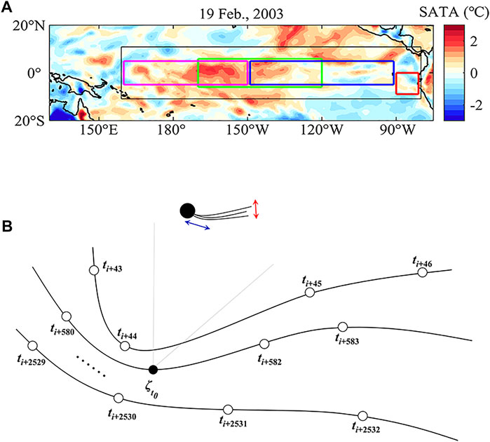
FIGURE 1. Illustration of the dynamical system analysis applied to the equatorial Pacific SATA. (A) Example of a real-time SATA map over the equatorial Pacific on 19 February 2003. The Niño1+2, Niño3, Niño4, and Niño3.4 regions are shown by red, blue, purple, and green boxes, respectively. The black box denotes the SATA field selected to construct the dynamical state space. (B) Idealized diagram of a trajectory in the dynamical state space of the SATA. A point ${\zeta }_{t_0}$ on this trajectory is encoded by the SATA latitude–longitude map at a certain time (as shown in Figure 1A). The zoomed sphere (black) shows the idealized schematic of the instantaneous persistence and dimension around ${\zeta }_{t_0}$.

In this study, we will utilize the Dynamical Systems metrics (DSMs, [17]) to analyze the spatiotemporal variability of the surface air temperature (SAT) over the tropical Pacific during El Niño episodes. DSM was proposed to quantify the instantaneous dynamical states of the climate subsystem over a given region, by incorporating both the spatial and temporal structures of the interested meteorological field. Different from the empirical orthogonal function (EOF), which relies on the linear covariance of the data, the DSM algorithm regards spatiotemporal data as the dynamical trajectory in the state space, and thus both linear and nonlinear statistical features can be characterized by DSM [13,17]. In recent studies, DSM has been applied to various issues in the climate study (e.g., [13,18–20]), where the instantaneous dynamical properties of the interested meteorological field can be effectively measured, and DSM is considered to be a promising tool to analyze the extreme events in the ocean and atmosphere.

Accordingly, two motivations of this study are to identify the dynamical properties of the SAT anomalies within different El Niño states and to interpret the physical meaning of DSM through analysis of the SAT over the tropical Pacific. On the one hand, the DSM applied to analyze SAT over tropical Pacific may address the aforesaid deficiency of Niño indices in the El Niño study. On the other hand, the interpretation of DSM could contribute further to a better understanding of this newly developed approach and provide a technical reference for future related climate studies.

The rest of this article is arranged as follow: Section 2 will describe the used data and DSM. Section 3 is divided into three parts: Section 3.1 will compare the Niño indices with the instantaneous dynamical parameters quantified by DSM, thus understanding how the dynamical states of SATA are influenced by the extreme events. Based on DSM, Section 3.2 will focus on the SAT anomaly (SATA) over the tropical Pacific during El Niño episodes, with regard to the diversity in spatial and temporal patterns of the SATA. Particularly, through analysis of the spatiotemporal patterns of SATA, the physical meaning of the DSM parameters in terms of the meteorological field will be demonstrated. Then, Section 3.3 will utilize the DSM parameters to compare different El Niño events. Further discussions and conclusions will be made in Section 4.

2 Data and Dynamical Systems Metrics

This study uses the daily mean 2-m temperature data (i.e., SAT) from the European Centre for Medium-Range Weather Forecasts’ ERA-Interim reanalysis [21], with a temporal range from 1979-01-01 to 2019-08-31. To focus on the anomalous variations of SAT, here, we subtract the long-term climatological average for each calendar day over the whole span from the 2-m temperature data. Additionally, the daily time series of Niño1+2, Niño3, Niño4, and Niño3.4 indices are obtained from the KNMI Climate Explorer website: http://climexp.knmi.nl. The spatial domains of Niño1+2, Niño3, Niño4, and Niño3.4 regions are, respectively, illustrated in Figure 1A. To cover these regions and measure the SATA dynamical states over the tropical Pacific, the spatial domain for the DSM computation is set at 160°E–80°W and 10°N–10°S (Figure 1A). Noting that DSM has been demonstrated to be not sensitive when the spatial resolution is set as 0.75°, 1.5°, and 2.5° [19], here, we select a horizontal resolution of 0.75° for the SATA data.

In the methodology of DSM [17], the evolution of a given meteorological field is acting as a dynamical system, in which the temporal evolutions of states of this dynamical system are described by an observed state-space trajectory X(t) (i.e., a matrix embedded with the spatiotemporal data). In this study, X(t) is a succession of daily SATA latitude–longitude maps within the selected spatial domain (see black box lines in Figures 1A), and a certain point ${\zeta }_{t_0}$ on this trajectory is a SATA latitude–longitude map for a specific day (Figure 1B).

Aiming at ${\zeta }_{t_0}$, we can infer the instantaneous dynamical property of the system at this specific day. The beginning step is to calculate the distance function $g\left(X\left(t\right),{\zeta }_{t_0}\right)=-\log \left[\mathrm{d}\mathrm{i}\mathrm{s}\mathrm{t}\left(X\left(t\right),{\zeta }_{t_0}\right)\right]$, in which “dist” represents the Euclidean distance between ${\zeta }_{t_0}$ and any other point on the trajectory $X\left(t\right)$. $g\left(X\left(t\right),{\zeta }_{t_0}\right)$ is a single-column matrix whose collected element takes large values when the point on the trajectory $X\left(t\right)$ is close to ${\zeta }_{t_0}$. Then, we can utilize this matrix to sort out the analogs of ${\zeta }_{t_0}$ on the state-space trajectory: by setting the top 98% quantile of $g\left(X\left(t\right),{\zeta }_{t_0}\right)$ as the threshold $s_X$, we retain the exceedances of $u\left(t, {\zeta }_{t_0}\right)=g\left(X\left(t\right),{\zeta }_{t_0}\right)–s_X$ but leave out the part at which $u\left(t,{\zeta }_{t_0}\right)<0$. It is noted that DSM is not sensitive to the choice of the quantile ranging from 90% to 99%. Thus, $u\left(t,{\zeta }_{t_0}\right)$ collects the analogs of ${\zeta }_{t_0}$, and its cumulative probability distribution $P\left[u\left({\zeta }_{t_0}\right)\right]$ satisfies the generalized Pareto distribution function as [17]:

$P\left[u\left({\zeta }_{t_0}\right)\right]\simeq \mathrm{e}\mathrm{x}\mathrm{p}\left[-\theta \left({\zeta }_{t_0}\right)\frac{u\left({\zeta }_{t_0}\right)}{\sigma \left({\zeta }_{t_0}\right)}\right].(1)$

As reported in the previous studies (19,22,23), the two parameters in Eq. 1 can be used to indicate the instantaneous dynamical properties of the system. $0<\theta \left({\zeta }_{t_0}\right)<1$ is interpreted as the inverse of instantaneous persistence: $\theta \left({\zeta }_{t_0}\right)$ taking lager values means that residence time of the system around ${\zeta }_{t_0}$ is shorter, while its low values denote the long residence time. Another derived parameter $d\left({\zeta }_{t_0}\right)=1/\sigma \left({\zeta }_{t_0}\right)$ is interpreted as the instantaneous dimension, denoting the degree of freedom of the system around ${\zeta }_{t_0}$. In terms of the SATA spatiotemporal field, the instantaneous persistence and dimension for each day are estimated, and then two time series ${\theta }_{SATA}\left(t\right)$ and $d_{SATA}\left(t\right)$ are obtained. The value of θ is estimated by using the Suveges likelihood estimator [24], and the programing code of d and θ are open access by Faranda et al. (see Data Availability Statement).

The aforementioned interpretations for the DSM parameters are in the sense of dynamical systems theory [18,23]; then, the recent studies have demonstrated that the values of instantaneous persistence and dimension are closely related to the intrinsic predictability of a certain climate subsystem ([19,20]). In this study, we will use ${\theta }_{SATA}\left(t\right)$ and $d_{SATA}\left(t\right)$ to investigate the underlying variations of the SATA dynamical states during El Niño episodes, and in turn the physical meaning of ${\theta }_{SATA}\left(t\right)$ and $d_{SATA}\left(t\right)$ in sense of the structural spatiotemporal patterns will be discussed.

3 Results

3.1 The Extreme Surface Air Temperature Anomaly States Measured by Dynamical Systems Metrics

We first analyze how the extreme SSTA states over the tropical Pacific influence the dynamical properties of SATA. The extreme SSTA states are usually inferred by referring to Niño indices. Though the four Niño indices are highly correlated to one another [5,14], extreme events from four different Niño indices are not completely consistent. For example, when the Niño1+2 index exceeds its 90% quantile, all of Niño3, Niño3.4, and Niño4 indices do not reach their own 90% quantiles (Figures 2A,B). This also means that extreme SSTA events can emerge from different sub-regions of the tropical Pacific [13]. Then, we observe how the dynamical properties of SATA vary with these extreme SSTA states defined by different Niño indices (Figures 2C,D). Niño1+2 and Niño4 indices denote the SSTA states in the eastern and western tropical Pacific, respectively (Figure 1A), and the comparison in Figure 2 shows that when either Niño1+2 index or Niño4 index reaches an extreme state, both ${\theta }_{SATA}$ and $d_{SATA}$ will all take their low values. This suggests that the extreme SSTA states over the tropical Pacific can increase the SATA persistence but decrease the SATA dimension.

FIGURE 2

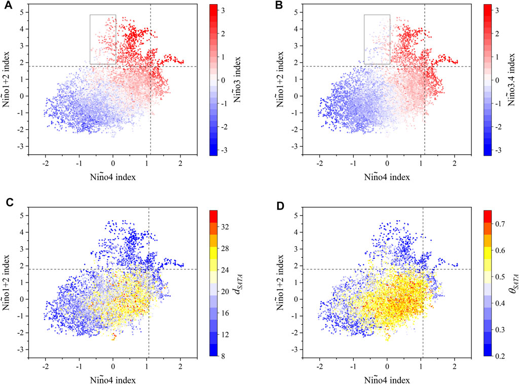
FIGURE 2. Comparisons among the four Niño indices and the dynamical properties of SATA. (A) Scatter plots of Niño1+2 index versus Niño4 index, and the color map of the Niño3 index. The dash lines denote the 90% quantiles of the Niño1+2 and Niño4 indices, respectively. (B) Same as (A), but the color map is for the Niño3.4 index. (C) Same as (A), but the color map is for $d_{SATA}$. (D) Same as (A), but the color map is for ${\theta }_{SATA}$.

Taking a segment of the SATA temporal evolution as an example (Figure 3), the covariation between DSM parameters and SATA spatiotemporal pattern can be observed. During the first 200 days of this segment, the zonal distribution of SATA is inhomogeneous and the SATA signals over different sub-regions are weak, at which ${\theta }_{SATA}$ and $d_{SATA}$ remain at high values. Since the 240th day of this segment, the central and eastern sub-regions of equatorial Pacific get anomalously warm, and at this time ${\theta }_{SATA}$ and $d_{SATA}$ start to decrease. During the days from 330 to 480 of this segment, the central and eastern sub-regions of the equatorial Pacific exhibit a consistent warm pattern, at which ${\theta }_{SATA}$ and $d_{SATA}$ remain at low values. This means that the persistence and dimension of SATA are closely related to the spatiotemporal pattern of SATA, and the low values of ${\theta }_{SATA}$ and $d_{SATA}$ may indicate the extreme states of SATA over the tropical Pacific. These results are reasonable. During the extreme SSTA events, the intensified air–sea interactions can cause the extreme SATA states [12,13], and the positive air–sea-coupled feedback can increase the persistence of the atmosphere over the tropical Pacific [13,25,26].

FIGURE 3

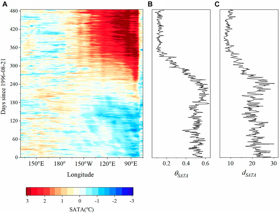
FIGURE 3. The SATA temporal evolution from 1996-08-21 to 1997-12-09. (A) SATA is averaged over 5°S–5°N as a function of time and longitude. (B) and (C) show the time series of ${\theta }_{SATA}$ and $d_{SATA}$.

3.2 Instantaneous Persistence and Dimension Within Different El Niño States

To further understand the association between the SATA dynamical properties and the different El Niño states, we inspect how ${\theta }_{SATA}$ and $d_{SATA}$ vary with the Niño3.4 index (Figure 4A). During 1981–2019, every time the Niño3.4 index exceeds its threshold (±0.5°C), the values of ${\theta }_{SATA}$ and $d_{SATA}$ will decrease. This is consistent with the result shown in Figure 3. However, the degree of changes in ${\theta }_{SATA}$ and $d_{SATA}$ is not identical during different El Niño events. Here, we mark five well-recognized CP and EP El Niño events [5,12,13] in Figure 4A, and it is obvious that the values of ${\theta }_{SATA}$ and $d_{SATA}$ in EP events are smaller than those in CP events. We then pick out all El Niño states by referring that the Niño3.4 index exceeds 0.5°C for at least five consecutive months and analyze these El Niño states in the scatter plot of ${\theta }_{SATA}$ versus $d_{SATA}$ (Figure 4B). The CP and EP El Niño states, respectively, cluster into two different groups in this scatter plot, and this means that the EP El Niño event can cause the stronger impact on the SATA dynamical properties than the CP.

FIGURE 4

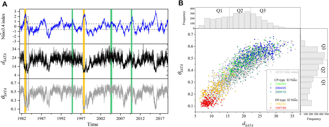
FIGURE 4. Analyses of the dynamical system parameters during El Niño episodes. (A) Time series of Niño34 index, $d_{SATA}$ and ${\theta }_{SATA}$. The dash lines across the Niño3.4 index denote the upper and lower threshold of ±0.5. The yellow and green bars indicate the typical EP and CP El Niño events (EP: 1982/83, 1997/98; CP: 1994/95, 2004/05, 2009/10). (B) Scatter plots of ${\theta }_{SATA}$ versus $d_{SATA}$ during El Niño days. Days within the typical EP and CP El Niño events are, respectively, illustrated. The histogram of ${\theta }_{SATA}$ is divided into the lowest 1/3 (Q1), the middle 1/3 (Q2), and the highest 1/3 (Q3) according to its quantiles, and so does $d_{SATA}$.

Focusing on the SATA dynamical properties during El Niño episodes (Figure 4B), ${\theta }_{SATA}$ and $d_{SATA}$ are found to vary widely, which corresponds to the variety of El Niño states and spatial warming patterns. We can further investigate these samples toward two informative aspects: the first one is to observe how spatiotemporal patterns of the SATA vary with the different El Niño states. The second one is an in-depth understanding in techniques, i.e., what the varied values of DSM parameters mean for the meteorological spatiotemporal field. Here, we divide these ${\theta }_{SATA}$ values into three groups: the smallest 1/3 (named ${\theta }_{Q1}$ group), the middle 1/3 (the ${\theta }_{Q2}$ group), and the largest 1/3 (the ${\theta }_{Q3}$ group), as the histogram of Figure 4B shows. Similarly, we also divide the samples of $d_{SATA}$ into three groups (i.e., the $d_{Q1}$, $d_{Q2}$, and $d_{Q3}$ groups) according to the three quantiles of the $d_{SATA}$ values. In the following, we will analyze the different groups of ${\theta }_{SATA}$ and $d_{SATA}$, respectively.

To show the spatiotemporal patterns of the SATA field corresponding to different values of ${\theta }_{SATA}$, here, we create the Hovmöller diagrams of SATA by, respectively, compositing the three groups (i.e., the ${\theta }_{Q1}$, ${\theta }_{Q2}$, and ${\theta }_{Q3}$ groups), as Figures 5A–C show. As the values of ${\theta }_{SATA}$ increase, the magnitudes of SATA along the equator decrease, and meanwhile the warming signal in the SATA field gets less persistent. We also utilize time-lagged correlation to analyze the persistence of SATA within these three groups. Taking the samples in the ${\theta }_{Q1}$ group as an example, we calculate spatial correlations between the SATA field at a certain day and its time-lagged ones (see Text. Supplementary Material S1) and then obtain the average result of the ${\theta }_{Q1}$ group, as shown in Figure 5D. Comparing the correlation curves of the three groups, it is found that as ${\theta }_{SATA}$ increases, the 1-day-lagged correlation coefficient decreases, and the correlation curve decays faster with time lags. The 90% confidence intervals of these three curves (Supplementary Figure S1) are clearly distinguishable from one another (i.e., confidence intervals are not overlapped with one another), which suggests that the SATA persistence magnitudes within these three groups are significantly different. Here, the results demonstrate that ${\theta }_{SATA}$ can seamlessly reflect the varying temporal persistence of the SATA field.

FIGURE 5

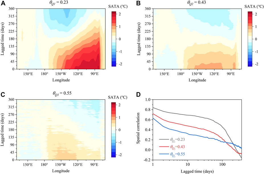
FIGURE 5. Comparison of the SATA Hovmöller diagrams between high and low persistence (during El Niño episodes). (A) SATA is averaged over 5°S–5°N as a function of the lag time and longitude, with compositing the days with the ${\theta }_{Q1}$ group (average of ${\theta }_{SATA}$: ${\theta }_{Q1}$ = 0.23). (B) Same as (A), but for the ${\theta }_{Q2}$ group (average of ${\theta }_{SATA}$: ${\theta }_{Q2}$ = 0.43). (C) Same as (A), but for the ${\theta }_{Q3}$ group (average of ${\theta }_{SATA}$: ${\theta }_{Q3}$ = 0.55). (D) Spatial correlation between the SATA field at a certain day and its time-lagged ones. The black line represents the average result for the ${\theta }_{Q1}$ group, red for the ${\theta }_{Q2}$ group, and blue for the ${\theta }_{Q3}$ group.

Toward the analysis on $d_{SATA}$, in Figure 6A, we composite the spatial patterns of SATA corresponding to three groups, respectively (i.e., the $d_{Q1}$, $d_{Q2}$, and $d_{Q3}$ groups). For the SATA spatial pattern of the $d_{Q1}$ group, both central and eastern regions of tropical Pacific get significantly warm, while only the central tropical Pacific gets warm for the $d_{Q3}$ group. This means that the low dimension corresponds to the more homogeneous spatial pattern of the meteorological field. Furthermore, we would investigate whether $d_{SATA}$ is also related to the synchrony of different grids in the SATA field, i.e., whether the temporal evolutions of the different grids are synchronized. Centered on a grid at the central Pacific (150°W, 0°), we calculate the cross-correlations of SATAs between other grids and this centered grid, in which results are derived for the three groups, respectively (Figure 6B). This result shows that the synchrony of this SATA field would decrease with the increased $d_{SATA}$. We also checked the cross-correlations by selecting different centered grids and found that the conclusion was not sensitive to the choice of the centered grid (Figure not shown here). These results demonstrate that $d_{SATA}$ can reflect whether the sub-regions of a meteorological field are consistently varying and to what degree the spatial pattern is homogeneous.

FIGURE 6

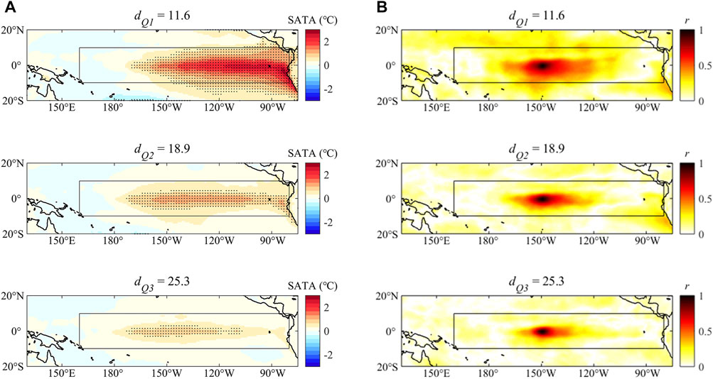
FIGURE 6. Comparison of the SATA patterns between high and low dimensions (during El Niño episodes). (A) Composite SATA patterns with (top panel) the $d_{Q1}$ group (average of $d_{SATA}$: $d_{Q1}$ = 11.6), (middle panel) the $d_{Q2}$ group (average of $d_{SATA}$: $d_{Q2}$ = 18.9), and (bottom panel) the $d_{Q3}$ group (average of $d_{SATA}$: $d_{Q3}$ = 25.3). (B) Same as (A), but for the cross-correlation (i.e., r) of SATAs between each grid and the grid at the central Pacific (150°W, 0°).

The aforementioned results interpret the physical meaning of ${\theta }_{SATA}$ and $d_{SATA}$ in the meteorological field, i.e., they characterize the variability of spatiotemporal patterns of SATA over the tropical Pacific. Moreover, the results shown in Figures 5, 6 demonstrate the impact of different El Niño states on the SATA spatiotemporal patterns. To observe the corresponding El Niño states, here, we further analyze the SST anomalies downloaded from NOAA High-resolution Blended Analysis of Daily SST dataset [27] and composite the SSTA spatial patterns of the $d_{Q1}$, $d_{Q2}$, and $d_{Q3}$ groups, respectively (Supplementary Figure S2). Corresponding to the $d_{Q1}$ group, the SSTs are found to be anomalously warm over the central and eastern regions of the tropical Pacific (Supplementary Figure S2A), while the $d_{Q3}$ group corresponds to the SSTA pattern at which only the central tropical Pacific gets warm (Supplementary Figure S2C). Since that ${\theta }_{SATA}$ and $d_{SATA}$ are highly correlated over the tropical Pacific (Figure 4B), the composite SSTA patterns for the ${\theta }_{Q1}$, ${\theta }_{Q2}$, and ${\theta }_{Q3}$ groups are similar to those for the three groups of $d_{SATA}$ (Figure not shown here). This reconfirms the conclusion obtained from Figure 4, i.e., the EP and CP types of El Niño can cause different impact on the persistence and dimension of the SATA field over the tropical Pacific.

3.3 Discriminating Different El Niño Events

The aforementioned section demonstrates that ${\theta }_{SATA}$ and $d_{SATA}$ can discriminate the different El Niño impacts on the SATA spatiotemporal patterns, and the impact is found to be related to the EP and CP types of El Niño states. In turn, we can employ ${\theta }_{SATA}$ and $d_{SATA}$ to further compare different El Niño events. In Figure 7A, we present the mean values of ${\theta }_{SATA}$ and $d_{SATA}$ within ten El Niño events during 1981–2019. In the scatter plot of ${\theta }_{SATA}$ versus $d_{SATA}$, the aforementioned typical EP and CP El Niño events are in two distinct divisions, among which the 2015/16 event is between these two divisions. In terms of magnitudes reflected by the Niño3.4 index (e.g., Figure 3A), the 2015/16 event is a super El Niño, and the corresponding SSTA pattern is close to an EP El Niño. However, recent studies found that the air–sea interactions and climate impact of the 2015/16 event are weaker than those of the typical EP El Niño [12,13,28,29]. Here, ${\theta }_{SATA}$ and $d_{SATA}$ confirm that the 2015/16 event has caused the weaker impact on the SATA spatiotemporal pattern than the EP El Niño but stronger than the CP ones. This result further confirms that the 2015/16 event may be a mixed-type El Niño.

FIGURE 7

FIGURE 7. Comparison of different El Niño events. (A) Scatter plots of ${\theta }_{SATA}$ versus $d_{SATA}$ in terms of the mean values during each El Niño event. (B) Scatter plots of Niño4 index versus Niño3 index in terms of the mean values during each El Niño event. The blue and red dots, respectively, indicate the typical EP and CP El Niño events.

The previous studies utilized the scatter plot of Niño3 and Niño4 indices to classify the types of El Niño [4,5,30]. For comparison, in Figure 7B, we present the mean values of Niño3 and Niño4 indices within the ten El Niño events. The diagonal line in this scatter plot can divide the typical EP and CP El Niño events into two divisions, whereas the events in 1986/87, 1991/92, 2006/07, and 2015/16 are close to the diagonal line. A similar phenomenon can be observed in the scatter plot of ${\theta }_{SATA}$ versus $d_{SATA}$ (Figure 7A), in which these four events are also between the divisions of EP and CP events. In the two kinds of scatter plots, the 2002/03 event is in the division of CP events, which is consistent with recent studies where this event is found to be closer to the CP type [12,31]. These results show that ${\theta }_{SATA}$ and $d_{SATA}$ can indeed discriminate different El Niño events.

4 Discussions and Conclusion

In this study, we employ the DSM parameters (i.e., ${\theta }_{SATA}$ and $d_{SATA}$) to quantify the El Niño impact on the SATA spatiotemporal patterns over the tropical Pacific. The results show that the extreme SSTA events can increase/decrease the persistence/dimension of SATA spatiotemporal patterns, and the impact of EP and CP El Niño events is different. Furthermore, we find that ${\theta }_{SATA}$ and $d_{SATA}$ can adequately discriminate different El Niño events (i.e., the EP, CP, and mixed-type events). This reconfirms that the El Niño impact on the atmosphere is closely related to the properties of events [12,13,31].

Additionally, in Section 3.2, we systematically discuss the physical meaning of ${\theta }_{SATA}$ and $d_{SATA}$ when they are applied to analyzing the meteorological field. ${\theta }_{SATA}$ denotes the persistence of the SATA patterns, while $d_{SATA}$ can reflect whether the sub-regions of the SATA field are consistently varying and to what degree the spatial pattern is homogeneous. This result can be useful for the future climate study when applying the DSM parameters.

In addition to El Niño, the extreme SSTA events over the tropical Pacific can be La Niña events, the coastal warming events, and the Pacific meridional mode events, etc. [4,13,32–34], but they are not analyzed in this study. From the results of DSM, it is shown that La Niña and the coastal warming events have also reduced the values of ${\theta }_{SATA}$ and $d_{SATA}$ (Figure 4A). Particularly, noting the dots marked by the black box lines in Figures 2A, 4A, these dots are explained by the 1983 coastal warming event [13,35]. Supplementary Figure S3 illustrates the spatiotemporal evolution of this event, compared with the time series of ${\theta }_{SATA}$ and $d_{SATA}$. During this event, most parts of the equatorial Pacific are not getting anomalously warm, but only the coastal areas are extremely warm, which is not the canonical El Niño. However, the time series of ${\theta }_{SATA}$ and $d_{SATA}$ show that the impact on SATA of this coastal warming event is comparable to that of the preceding El Niño event (Supplementary Figures S3B, S3C). This is in line with the previous studies about the extreme impact of coastal warming events on the weather and climate [13,35]. These results further confirm that the DSM parameters can faithfully quantify the impact of these extreme events, and the wide application of this method and the relevant extreme events deserve an in-depth study in the future. The current article only focuses on the DSM-based analysis of the El Niño events during 1981–2019; the more detailed studies for different kinds of extreme SSTA events, including their potential changes in the future climate change scenarios, will be addressed in our following work.

Data Availability Statement

The original contributions presented in the study are included in the article/Supplementary Material; further inquiries can be directed to the corresponding author.

Author Contributions

YH and ZF designed the study. YH accomplished the computations. YH wrote the manuscript. All authors discussed and interpreted the results and edited the manuscript.

Funding

This work was supported by the National Natural Science Foundation of China (Nos. 42175065 and 41975059).

Conflict of Interest

The authors declare that the research was conducted in the absence of any commercial or financial relationships that could be construed as a potential conflict of interest.

Publisher’s Note

All claims expressed in this article are solely those of the authors and do not necessarily represent those of their affiliated organizations, or those of the publisher, the editors, and the reviewers. Any product that may be evaluated in this article, or claim that may be made by its manufacturer, is not guaranteed or endorsed by the publisher.

Acknowledgments

The authors thank the constructive suggestions of the reviewers.

Supplementary Material

The Supplementary Material for this article can be found online at: https://www.frontiersin.org/articles/10.3389/fphy.2022.919951/full#supplementary-material

References

1. Timmermann A, An S-I, Kug J-S, Jin F-F, Cai W, Capotondi A, et al. El Niño-Southern Oscillation Complexity. Nature (2018) 559(7715):535–45. doi:10.1038/s41586-018-0252-6

PubMed Abstract | CrossRef Full Text | Google Scholar

2. Cai W, Wu L, Lengaigne M, Li T, McGregor S, Kug JS, et al. Pantropical Climate Interactions. Science (2019) 363(6430):944. doi:10.1126/science.aav4236

PubMed Abstract | CrossRef Full Text | Google Scholar

3. Hu ZZ, McPhaden MJ, Kumar A, Yu JY, Johnson NC. Uncoupled El Niño Warming. Geophys Res Lett (2020) 47(7):e2020GL087621. doi:10.1029/2020gl087621

CrossRef Full Text | Google Scholar

4. Kug J-S, Jin F-F, An S-I. Two Types of El Niño Events: Cold Tongue El Niño and Warm Pool El Niño. J Clim (2009) 22(6):1499–515. doi:10.1175/2008jcli2624.1

CrossRef Full Text | Google Scholar

5. Ren HL, Jin FF. Niño Indices for Two Types of ENSO. Geophys Res Lett (2011) 38:L04704. doi:10.1029/2010gl046031

CrossRef Full Text | Google Scholar

6. Capotondi A, Wittenberg AT, Newman M, Di Lorenzo E, Yu J-Y, Braconnot P, et al. Understanding ENSO Diversity. Bull Am Meteorol Soc (2015) 96(6):921–38. doi:10.1175/bams-d-13-00117.1

CrossRef Full Text | Google Scholar

7. Gill AE. Some Simple Solutions for Heat-Induced Tropical Circulation. Q.J R Met. Soc. (1980) 106(449):447–62. doi:10.1002/qj.49710644905

CrossRef Full Text | Google Scholar

8. Williams IN, Patricola CM. Diversity of ENSO Events Unified by Convective Threshold Sea Surface Temperature: a Nonlinear ENSO index. Geophys Res Lett (2018) 45(17):9236–44. doi:10.1029/2018gl079203

CrossRef Full Text | Google Scholar

9. Horel JD, Wallace JM. Planetary-scale Atmospheric Phenomena Associated with the Southern Oscillation. Mon Wea Rev (1981) 109(4):813–29. doi:10.1175/1520-0493(1981)109<0813:psapaw>2.0.co;2

CrossRef Full Text | Google Scholar

10. Meng J, Fan J, Ashkenazy Y, Havlin S. Percolation Framework to Describe El Niño Conditions. Chaos (2017) 27(3):035807. doi:10.1063/1.4975766

PubMed Abstract | CrossRef Full Text | Google Scholar

11. Hou Z, Li J, Ding R, Karamperidou C, Duan W, Liu T, et al. Asymmetry of the Predictability Limit of the Warm ENSO Phase. Geophys Res Lett (2018) 45(15):7646–53. doi:10.1029/2018gl077880

CrossRef Full Text | Google Scholar

12. Lu ZH, Yuan NM, Chen L, Gong Z. On the Impacts of El Niño Events: a New Monitoring Approach Using Complex Network Analysis. Geophys Res Lett (2020) 47(6):e2019GL086533. doi:10.1029/2019gl086533

CrossRef Full Text | Google Scholar

13. Huang Y, Yuan N, Shi M, Lu Z, Fu Z. On the Air-Sea Couplings over Tropical Pacific: An Instantaneous Coupling index Using Dynamical Systems Metrics. Geophys Res Lett (2022) 49(2):e2021GL097049. doi:10.1029/2021gl097049

CrossRef Full Text | Google Scholar

14. Trenberth KE, Stepaniak DP. Indices of El Niño Evolution. J Clim (2001) 14(8):1697–701. doi:10.1175/1520-0442(2001)014<1697:lioeno>2.0.co;2

CrossRef Full Text | Google Scholar

15. Song W-J, Yu J-Y. Identifying the Complex Types of Atmosphere-Ocean Interactions in El Niño. Environ Res Lett (2019) 14(11):114030. doi:10.1088/1748-9326/ab4968

CrossRef Full Text | Google Scholar

16. Ren HL, Wang R. Distinct Growth Rates of the Two ENSO Types. Geophys Res Lett (2020) 47(16):e2020GL088179. doi:10.1029/2020gl088179

CrossRef Full Text | Google Scholar

17. Faranda D, Messori G, Yiou P. Diagnosing Concurrent Drivers of Weather Extremes: Application to Warm and Cold Days in North America. Clim Dyn (2020) 54(3-4):2187–201. doi:10.1007/s00382-019-05106-3

CrossRef Full Text | Google Scholar

18. Messori G, Caballero R, Faranda D. A Dynamical Systems Approach to Studying Midlatitude Weather Extremes. Geophys Res Lett (2017) 44(7):3346–54. doi:10.1002/2017gl072879

CrossRef Full Text | Google Scholar

21. Dee DP, Uppala SM, Simmons AJ, Berrisford P, Poli P, Kobayashi S, et al. The ERA-Interim Reanalysis: Configuration and Performance of the Data Assimilation System. Q.J.R Meteorol Soc (2011) 137(656):553–97. doi:10.1002/qj.828

CrossRef Full Text | Google Scholar

19. Faranda D, Messori G, Yiou P. Dynamical Proxies of North Atlantic Predictability and Extremes. Sci Rep (2017) 7:41278. doi:10.1038/srep41278

PubMed Abstract | CrossRef Full Text | Google Scholar

22. Faranda D, Masato G, Moloney N, Sato Y, Daviaud F, Dubrulle B, et al. The Switching between Zonal and Blocked Mid-latitude Atmospheric Circulation: a Dynamical System Perspective. Clim Dyn (2016) 47(5):1587–99. doi:10.1007/s00382-015-2921-6

CrossRef Full Text | Google Scholar

23. Faranda D, Vaienti S. Correlation Dimension and Phase Space Contraction via Extreme Value Theory. Chaos (2018) 28(4):041103. doi:10.1063/1.5027386

PubMed Abstract | CrossRef Full Text | Google Scholar

24. Süveges M. Likelihood Estimation of the Extremal index. Extremes (2007) 10:41–55.

Google Scholar

20. Faranda D, Alvarez-Castro MC, Messori G, Rodrigues D, Yiou P. The Hammam Effect or How a Warm Ocean Enhances Large Scale Atmospheric Predictability. Nat Commun (2019) 10(1):1316. doi:10.1038/s41467-019-09305-8

PubMed Abstract | CrossRef Full Text | Google Scholar

25. Zheng F, Fang X-H, Yu J-Y, Zhu J. Asymmetry of the Bjerknes Positive Feedback between the Two Types of El Niño. Geophys Res Lett (2014) 41(21):7651–7. doi:10.1002/2014gl062125

CrossRef Full Text | Google Scholar

26. Bach E, Motesharrei S, Kalnay E, Ruiz-Barradas A. Local Atmosphere-Ocean Predictability: Dynamical Origins, lead Times, and Seasonality. J Clim (2019) 32(21):7507–19. doi:10.1175/jcli-d-18-0817.1

CrossRef Full Text | Google Scholar

27. Reynolds RW, Smith TM, Liu C, Chelton DB, Casey KS, Schlax MG. Daily High-Resolution-Blended Analyses for Sea Surface Temperature. J Clim (2007) 20(22):5473–96. doi:10.1175/2007jcli1824.1

CrossRef Full Text | Google Scholar

28. Paek H, Yu JY, Qian CC. Why Were the 2015/2016 and 1997/1998 Extreme El Niños Different? Geophys Res Lett (2017) 44(4):1848–56.

Google Scholar

29. Hu S, Fedorov AV. Cross-equatorial Winds Control El Niño Diversity and Change. Nat Clim Change (2018) 8(9):798–802. doi:10.1038/s41558-018-0248-0

CrossRef Full Text | Google Scholar

30. Yeh S-W, Kug J-S, Dewitte B, Kwon M-H, Kirtman BP, Jin F-F. El Niño in a Changing Climate. Nature (2009) 461(7263):511–4. doi:10.1038/nature08316

PubMed Abstract | CrossRef Full Text | Google Scholar

31. Okumura YM. ENSO Diversity from an Atmospheric Perspective. Curr Clim Change Rep (2019) 5(3):245–57. doi:10.1007/s40641-019-00138-7

CrossRef Full Text | Google Scholar

32. Zhao J, Kug JS, Park JH, An SI. Diversity of North Pacific Meridional Mode and its Distinct Impacts on El Niño-Southern Oscillation. Geophys Res Lett (2020) 47(19):e2020GL088993. doi:10.1029/2020gl088993

CrossRef Full Text | Google Scholar

33. Pietri A, Colas F, Mogollon R, Tam J, Gutierrez D. Marine Heatwaves in the Humboldt Current System: from 5-day Localized Warming to Year-Long El Niños. Sci Rep (2021) 11(1):21172. doi:10.1038/s41598-021-00340-4

PubMed Abstract | CrossRef Full Text | Google Scholar

34. Shi M, Huang Y, Fu Z. Dynamical Systems Persistence Parameter of Sea Surface Temperature and its Associations with Regional Averaged index over the Tropical Pacific. Intl J Climatology (2022). doi:10.1002/joc.7664

CrossRef Full Text | Google Scholar

35. Hu Z-Z, Huang B, Zhu J, Kumar A, McPhaden MJ. On the Variety of Coastal El Niño Events. Clim Dyn (2019) 52(12):7537–52. doi:10.1007/s00382-018-4290-4

CrossRef Full Text | Google Scholar