 Justin R. Rippy
 Manmohan Singh1
 Salavat Aglyamov
 Kirill V. Larin
95% of researchers rate our articles as excellent or good
Learn more about the work of our research integrity team to safeguard the quality of each article we publish.
Find out more
ORIGINAL RESEARCH article
Front. Phys. , 24 June 2022
Sec. Medical Physics and Imaging
Volume 10 - 2022 | https://doi.org/10.3389/fphy.2022.917842
This article is part of the Research Topic Innovative Developments in Multi-Modality Elastography View all 20 articles
Tissue stiffness is a key biomechanical property that can be exploited for diagnostic and therapeutic purposes. Tissue stiffness is typically measured quantitatively via shear wave elastography or qualitatively through compressive strain elastography. This work focuses on merging the two by implementing an uncalibrated stress sensor to allow for the calculation of Young’s modulus during compression elastography. Our results show that quantitative compression elastography is able to measure Young’s modulus values in gelatin and tissue samples that agree well with uniaxial compression testing.
In modern medicine, diagnostic and treatment decisions are becoming increasingly influenced by measurements of biomechanical properties of tissues. This is especially true in the fields of oncology [1], dermatology [2], and hepatology [3]. Because disease states necessarily involve the physical change of the affected tissue, biomechanical properties are often a good indicator of both disease presence and extent.
A key biomechanical property that is most often measured in clinical use is tissue stiffness. Changes in tissue structure on the microscale result in changes in tissue stiffness on the macroscale. For example, tumors often vary in stiffness from the surrounding tissue. Subsequently, tumor stiffness can be used to detect tumors [4], aid in staging them [5], determine their metastatic potential [6], and aid in the evaluation of treatment [7]. Similarly, a liver disease resulting in fibrosis or steatosis can be diagnosed via liver stiffness measurement [3, 8]. Treatment of many diseases in addition to the aforementioned diseases involving soft tissues, can benefit from the analysis of tissue stiffness for diagnostic and therapeutic planning and evaluation.
The field of elastography is generally focused on the measurement of tissue stiffness via various imaging modalities. For superficial or excised tissues, this can be accomplished with noninvasive optical techniques such as optical coherence elastography (OCE) [9–11], which can provide high-resolution elastograms. However, due to light attenuation in tissue, optical-based elastography methods cannot be used in tissues that are deeper than a few mm beneath the surface unless an invasive probe is utilized [12]. Magnetic resonance elastography (MRE) does not have this limitation and is used to make whole-organ and whole-body elasticity maps but suffers from relatively poor resolution, typically in the mm range [13]. Additionally, it is expensive and requires a large amount of space. A third option is ultrasound elastography [14], which is portable, comparatively inexpensive, and has been practiced the longest and studied the most of the three techniques. It can offer both deep tissue penetration and high resolution, though there is a tradeoff between these two factors. Ultrahigh-frequency ultrasound transducers with frequencies in the hundreds of MHz are capable of approaching optical imaging resolution both axially and laterally at the cost of penetration depth; however, these are still at an early stage and are currently manufactured in laboratories for use in experimental setups [15]. Elastography is typically performed at lower frequencies (< 5 MHz), resulting in resolutions of hundreds of microns up to mm scale [15].
The two main branches of ultrasound elastography are static/quasi-static compressive strain elastography [16, 17] and shear wave elastography [18, 19]. In strain elastography, a series of images are taken as the tissue is slowly compressed, which results in a measure of how the strain distribution changes with compression. This method typically results in semi-quantitative measurements and shows the ratio between the strains in different regions. Because of the manual compression, there can be high operator error and low repeatability [20], which is compounded by the nonlinear biomechanical properties of tissues [21]. Shear wave elastography, on the other hand, involves inducing a mechanical wave inside the tissue and measuring its speed. This allows for a quantitative measurement based upon the shear wave speed, i.e., shear modulus or Young’s modulus. These mechanical parameters are absolute measurements of tissue elasticity and are more valuable because they allow for comparisons between different time points during the treatment of a single patient, between different patients, and between different diseases. Strain-based compressive elastography can also obtain absolute Young’s modulus in tissues but requires the use of a precisely calibrated compliant sensor for measurements of surface stress, which has been utilized widely in optical coherence micro-elastography [22, 23]. However, use of a stress sensor in ultrasound elastography is not as prominent as in optical methods.
In this work, we combine strain and shear wave elastography using a stress sensor placed on the sample to obtain two-dimensional quantitative stiffness maps in a new technique called quantitative compression elastography (QCE). Unlike quantitative micro-elastography, our method does not require a calibrated sensor with precisely known mechanical characteristics. Instead, shear waves are generated within the sensor, which can be converted to quantitative elastic modulus values. Using these values and the strains measured within the sensor and the tissue of interest, we measure quantitative tissue stiffness values. We also compare these values to uniaxial compression testing (UT) for validation. To our knowledge, this is the first translation of strain imaging in ultrasound elastography to the quantitative mapping of biomechanical properties through the use of an uncalibrated stress sensor.
The experimental setup is shown in Figure 1. It consists of a Vantage 256 (Verasonics, Kirkland, WA, United States) ultrasound system with an L11-5 V transducer. The imaging and push frequencies were 7.8 MHz and the pulse duration was 128 μs. The transducer was placed into a custom holder to ensure stability and prevent movement. Each sample was placed on a linear z-axis stage which served to produce the compression. Ultrasound gel was degassed using a vacuum chamber and a thin layer was placed between the ultrasound transducer and the sample. The transducer was placed above the surface of the sample and guided into place by raising the z-axis stage.
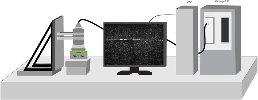
FIGURE 1. The experimental setup, consisting of a custom probe mount, Verasonics Vantage 256 system, and a z-axis stage. The transducer is held firmly in place as the z-axis stage is incrementally raised to compress the sample, during which shear wave and compression data is obtained.
Gelatin phantoms were created by mixing gelatin (gel strength 300, type A. Sigma-Aldrich Corp, MO, United States) with distilled water and pouring it into a cylindrical mold with a diameter of approximately 8 cm. Silica powder was added to all phantoms and sensors to promote acoustic scattering and to make the boundaries easy to visualize on ultrasound imaging. Prior to measurement, all phantoms were removed from their molds via a custom lift mechanism to avoid tearing the phantom. This lift mechanism consists of a circular piece of thin acrylic cut with a laser cutter to match the diameter of the cylindrical mold. Two thin strips of metal were bent at a 90-degree angle and glued to the bottom of the acrylic to allow for the whole acrylic disk and the solidified phantom to be lifted as a single unit. When possible, the sensor was created by pouring the sensor gelatin mixture on top of the sample to avoid acoustic impedance mismatch that could create artifacts in the presence of an air gap or the insertion of bubbles. For each concentration, a separate small cylindrical phantom with a diameter of approximately 3.5 cm was also cast for validation via uniaxial mechanical compression testing.
Homogeneous phantoms with concentrations of approximately 10% gelatin (w/w) and 16% gelatin (w/w) were created. Silica powder at a concentration of approximately 0.8% (w/w) was added for scattering. They were poured into the aforementioned cylindrical mold allowed to solidify. A sensor layer of 9% gelatin (w/w) containing 0.5% silica powder (w/w) with a thickness of approximately 4 mm was poured on top and allowed to solidify.
A half and half phantom was created to assess the capability of the technique to assess spatial variations in stiffness. Half of the phantom consisted of 16% gelatin (w/w) with 0.8% silica powder (w/w), and the other half was 10% gelatin (w/w) with 0.6% silica powder (w/w). The silica powder was varied to allow for visualization of the boundary between the halves. The gelatin was poured into the aforementioned cylindrical mold, allowed to solidify. A sensor layer of 9% gelatin (w/w) with 0.4% silica powder (w/w) with a thickness of approximately 4 mm was poured on top and allowed to solidify.
Beef steak was acquired fresh from a local grocery store and cut into a small strip of approximately 5 cm by 10 cm. Half of the sample was cooked on a hot plate at 150°C for ∼1–2 min per side to change the local biomechanical properties of the region. Both sides of the cooked region were heated to ensure biomechanical changes were consistent through the entire depth, and the tissue was allowed to cool to room temperature before measurements. An image of the tissue is shown in Figure 2, which clearly shows the delineation between the cooked and uncooked regions. When placed under the transducer, a copper wire was aligned with the visible cooked boundary for visualization on the ultrasound B-mode image before a 16% gelatin (w/w) sensor with a thickness of approximately 5 mm was placed on top. Prior to the acquisition, the wire was carefully removed from beneath the sensor.
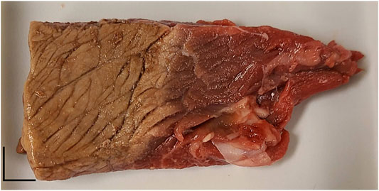
FIGURE 2. Photograph of the steak sample. The left side was cooked and the right side was uncooked. The boundary can be clearly seen in the middle. The scale bar is approximately 1 cm in each direction.
Phantoms of each concentration underwent uniaxial mechanical compression testing (Model 5,943, Instron Corp, Norwood, MA, United States) to measure Young’s modulus by the “gold standard” for comparison. The height and radius of the cylindrical phantoms were measured with digital calipers, and the sample was coated with water to prevent friction between the compression testing frame plates. After coming into contact with the phantom, the test began and continued until either 20% strain or 50 N of force was reached. Compression was performed at 0.25 mm/s. The phantom was removed, and rewet after each measurement, and a total of five measurements were performed on each sample.
The raw mechanical testing data was loaded into MATLAB (Mathworks, Inc., Natick, MA, United States), and stress and strain were calculated using the measured dimensions of the phantom. A polynomial best fit line to the stress-strain curve was obtained, and the derivative was calculated. This derivative equation corresponded to the tangent Young’s modulus as a function of strain and was used for validation of the ultrasound compression elastography method.
Custom acquisition software was written in MATLAB to control the Vantage 256 system in conjunction with the z-stage. For each compression position, 120 plane-wave ultrasound images were taken and saved as IQ data. Following this, a shear wave was generated approximately 0.5 mm below the sensor layer, and an additional 120 plane-wave ultrasound images were taken to monitor the wave as it passed through the sensor and sample. An image was taken every 100 µs. The shear wave was generated by using 32 elements of the transducer, and the apodization and delays were calculated via software provided by the ultrasound manufacturer. This ensured that the wavefronts from each transducer element arrived at the shear wave excitation focal point at the appropriate time to generate a shear wave. The z-stage was raised by 100 μm, and the process was repeated until the desired number of compressions was reached.
A flow chart of the processing steps is shown in Figure 3. The shear wave data sets were processed as follows. First, the particle velocity was obtained in each of the 120 frames using the vector method [24] with a kernel size of 20 pixels, which corresponded to 1.35 µm. The particle velocity, i.e., the temporal derivative of the displacement in the axial direction, for each pixel was summed in time to obtain displacement in each frame. Then, the displacement images were smoothed using a Savitzky-Golay filter with polynomial order of one and a frame length of 21. The data were interpolated in time by a factor of 5. The Fourier transform of the displacement data in time was taken at the level of the sensor in the path of wave propagation to determine the frequencies corresponding to the shear wave. The displacement data stack was then bandpass filtered to isolate the frequencies corresponding to the shear wave. A cross correlation-based method was utilized to obtain the temporal lags of the wave propagation in the sensor. A shear wave speed map was generated from the wave propagation time lags and spatial coordinates using a sliding window with a kernel size of approximately 1.69 mm.
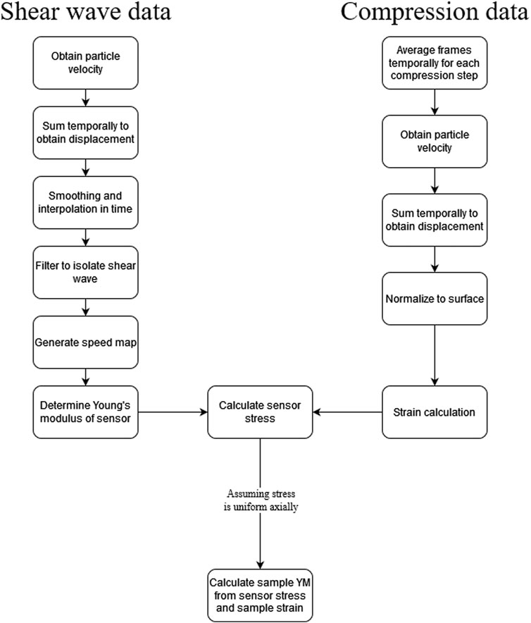
FIGURE 3. Flow chart depicting the data processing steps.
The compression data was processed as follows. The IQ data for each compression data set was loaded, and the 120 frames were averaged in time to remove noise for each compression step. The result was a stack containing complex B-scan images of the sensor and sample. The complex images were converted to intensity grayscale images, which were then segmented using MATLAB’s volumeSegmenter tool. The vector method was used on the complex image stack to generate particle velocity maps, which were then cumulatively summed in time to generate displacement maps. Following this, each displacement image was normalized such that the displacement at the interface between the sensor and the transducer was zero. The strain was calculated from the displacement frame by using the least-squares regression fit of the axial displacement with a window size of approximately 0.225 mm [25].
The Young’s modulus of the sensor was calculated from the speed of the shear wave. The area of the excitation pulse was removed to avoid near-field effects, which overestimates the velocity of the waves generated in or near the shear wave excitation focal point. The wave speed map of the sensor was converted to Young’s modulus, E, via the following relationship [10]:
where ρ was the mass density of the sensor material and
The stress in the sensor was then calculated via the following relationship:
where σ was the stress in the sensor and ε was the strain in the sensor. Assuming that the stress was uniform axially between the two rigid boundaries of the setup, i.e., the transducer and lower plate, Young’s modulus was computed for each pixel in the strain map of the sample by
The resulting images were then smoothed via cubic spline interpolation. The average of the segmented area was then taken after outliers were removed to obtain the final average Young’s modulus value for the sample or region of interest.
The results from the homogeneous phantoms are shown in Figure 4 and in Table 1. For the 10% phantom, the average value was 22.36 ± 1.59 kPa, and the average for the 16% phantom was 41.39 ± 3.15 kPa. The slope of the stress-strain curve from uniaxial testing resulted in Young’s modulus of 22.73 kPa for the 10% phantom and 40.14 kPa for the 16% phantom. The average percent errors for the 10% phantom and 16% phantom were 5.91% and 6.68%, respectively. The results from the half and half gelatin phantom are shown in Figure 5. For the softer side, the average value of the measurements using the ultrasound compression method was 23.33 ± 1.66 kPa. The slope of the stress-strain curve from uniaxial testing resulted in Young’s modulus of 23.01 kPa. Overall, there was an average percent error of 5.60% by QCE as compared to mechanical testing. For the stiffer side, the average elasticity was 40.83 ± 1.75 kPa as measured by compression elastography. The slope of the stress-strain curve from mechanical testing was 41.44 kPa. Overall, there was an average percent error of 3.98% by QCE as compared to mechanical testing.
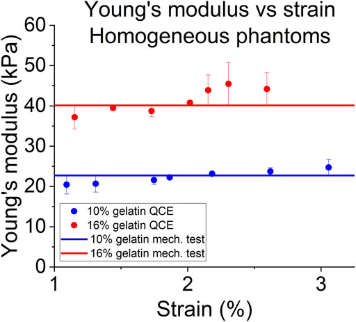
FIGURE 4. Young’s modulus as a function of compressive strain of QCE and mechanical testing for homogeneous phantoms.
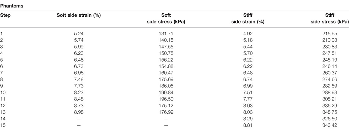
TABLE 1. Values of stress and strain for the soft and stiff sides of the phantom experiment.
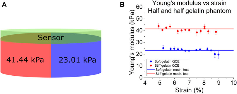
FIGURE 5. (A) Schematic and uniaxial mechanical compression testing (mech. test) measurements of the half and half gelatin phantom. (B) Young’s modulus as a function of the compressive strain of QCE and mechanical testing.
The measured elasticity values for the tissue sample can be seen in Figure 6 and in Table 2. The elasticity of the uncooked steak increased from 16.25 kPa to 31.84 kPa over a compressive range of 4.94%–8.87%, as estimated by QCE. Mechanical testing measured Young’s modulus of the uncooked steak as 14.61–38.66 kPa over the same region. Overall, there was an average percent error of 6.06% by QCE as compared to mechanical testing. The elasticity of the cooked steak increased from 11.79 to 25.62 kPa over a compressive range of 0.5%–9.01%, as estimated by QCE. Mechanical testing measured Young’s modulus of the cooked steak as 13.64 to 28.95 over the same region. Overall, there was an average percent error of 5.59% by QCE as compared to mechanical testing.
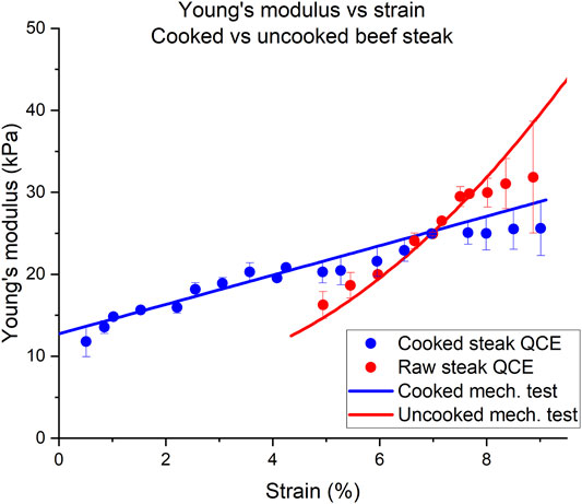
FIGURE 6. Tangent Young’s modulus (YM) as a function of compressive strain for a half-cooked beef steak. The red and blue circles indicate Young’s modulus estimated for the cooked and uncooked halves of the steak using QCE, respectively. The solid lines were obtained from the slope of the stress-strain curve obtained from mechanical testing.
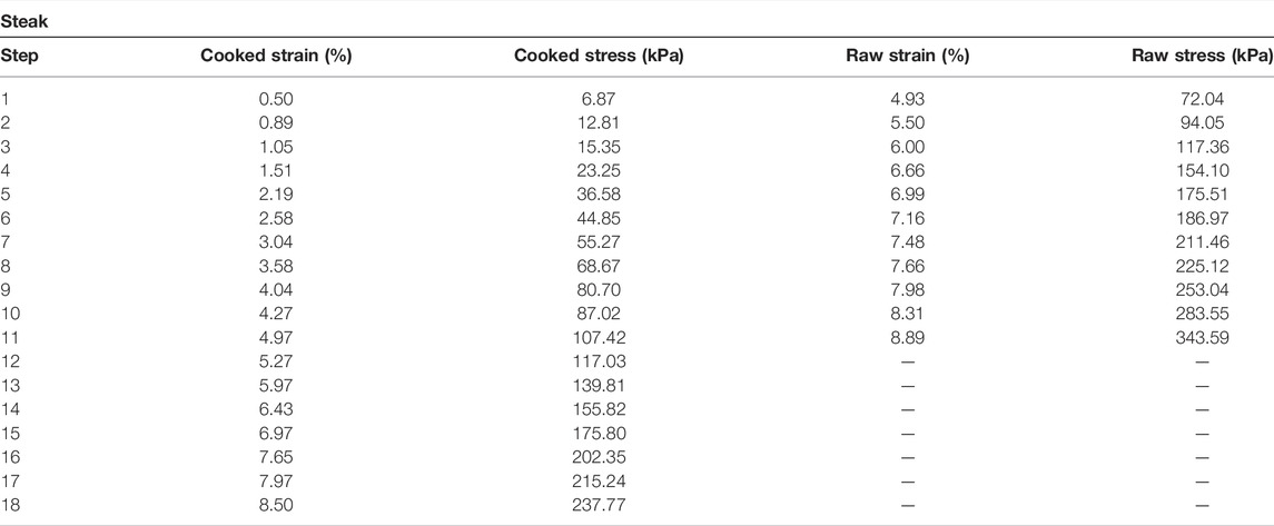
TABLE 2. Values of stress and strain for the cooked and uncooked sides of the steak experiment.
For the strain ranges shown, the cooked half of the steak had a much more linear slope with increasing compression than the uncooked half of the steak. The solid blue line is the derivative used to approximate the stress-strain curve of the uniaxial testing data. The raw tissue did not have a linear trend of tangent Young’s modulus beyond ∼7%. The mechanical testing uniaxial data is plotted in Figure 6 as the solid red and blue lines for the uncooked and cooked steak, respectively.
Our results show good agreement between Young’s modulus measured with QCE and Young’s modulus measured by uniaxial testing. These results validate QCE as a simple, multimodal, accessible, and relatively low-tech method to obtain quantitative information on tissue stiffness.
Gelatin was chosen because, for small strains, Young’s modulus is approximately constant as a function of strain [26, 27]. Some studies have shown an approximately linear stress-strain curve up to approximately 20% strain [28]. We found that this remained a good approximation in the strain region we considered, which was below 10% strain. When measuring the homogeneous phantoms, the errors remained below 7% when compared to uniaxial compression testing. When estimating the elasticity of each side of the heterogeneous phantom using QCE, the errors remained below 6% as compared to uniaxial mechanical compression testing, indicating that QCE is capable of a high degree of accuracy for tissue stiffness assessment.
Hooke’s law is valid only in the case of materials with linear-elastic behavior; i.e., in situations where the stress-strain curve is linear. Here, we assume that we are within the linear-elastic region, that the strain increases slowly, and that there is no permanent modification to the material.
The tangent Young’s modulus values measured in the tissue sample (steak) via QCE were in good agreement with mechanical testing as well. There was a significant preload on the raw side prior to elastography measurements being taken. This is because the tissue shrank during cooking, and thus, the initial strain on the thicker uncooked side was greater as compared to the thinner, cooked side. Though the raw and cooked tissues were under different loads during the experiment, accurate results were still obtained without the use of a calibrated stress sensor. As in the gelatin phantom, the error remained low at ∼6%, proving further that QCE is able to accurately measure tissue stiffness.
The tissue did not exhibit linear elasticity, which is as expected [21, 29, 30]. While most tissues show strain hardening, this behavior varies by tissue type [31, 32]. This is characterized by a large initial compression with low levels of stress followed by strain hardening, where the stress increases in a nonlinear fashion with increasing strain [31, 33]. The raw tissue exhibited this to a greater degree than the cooked tissue, but QCE can accurately measure tissue stiffness regardless of whether it is in the linear or nonlinear regime since the stress measurements are made for a given strain.
Typically, to perform quantitative strain elastography, a compliant sensor with precisely known properties is needed [22, 23]. This involves uniaxial testing beforehand to measure these properties and precise measurements of the pre-stress before imaging. Uniaxial testing machines are expensive and are unlikely to be found in most hospitals or clinical settings, unlike ultrasound imaging systems. Additionally, if the sensor breaks or needs to be changed, calibration must again be performed on the sensor, which is particularly noteworthy in cases where sterility is necessary. One major novelty of the presented method is that it eliminates the need for the calibration step. The sensor need only be linear in the strain region that will be utilized in the sensor and sufficiently scattering to visualize shear wave propagation. If the sensor enters the nonlinear region, the elasticity is no longer accurately estimated by Eqs 4–1, which means that Young’s modulus value will not be correct. An alternative form of the relationship in Eq. 3 shows the problem more clearly:
If
An additional constraint on the sensor is that it must not be too soft or stiff. If the sensor is too soft, then during compression, most of the deformation will go into the sensor instead of being distributed between the sensor and sample, and there will be no measurable strain in the sample. If the sensor is too stiff, it will not deform during compression, and there will be no measurable strain and, thus, stress. In both cases, the method will likely fail due to the lack of a measurable strain. The strain must be accurately measured in both the sensor and the sample for this method to be successful. In the clinic, acoustic coupling gel is often used, but acoustic coupling gel pads are also commercially available, which may serve as stress sensors. One such gel pad is Aquaflex, which has been studied previously [34] and is widely available. However, their mechanical properties are not often known, and thus, this technique would be useful in such use cases assuming the stiffness of the gel pad is not too low or high. One difficulty in using commercial gel pads is that they are designed to be acoustically transparent, which would limit visualization of the shear wave propagation and, therefore, the estimation of shear wave speed. A commercially manufactured gel pad with a low concentration of acoustic scatterers would be preferable for this application.
Clinical ultrasound imaging machines typically do not allow the transducer to act as a shear wave source, which means that this method cannot be used in those settings. Though it is most convenient when the transducer can act as both a shear wave generator and an imaging modality, this method could be performed with an additional wave source, such as a mechanical actuator utilized in MRE [35]. The main concern is that wave propagation with a sufficient signal-to-noise ratio [36] must be observed in the sensor.
Shear wave propagation in the sample is not necessary when using this method. This means that the method can work for any deformable tissue even in the presence of high dispersion or attenuation, provided that strain in the tissue can be accurately measured. If the underlying structure is not deformed enough, then strain cannot be determined, and therefore the value of
Two key processing steps have the potential to change the accuracy of QCE. First is the estimation of the shear wave speed in the sensor. If the speed in the sensor is poorly estimated due to poor wave propagation, poor scattering, or other factors limiting wave propagation or its detection, then the accuracy of this method will decrease. The algorithm with which speed is estimated also determines accuracy to some degree. If using windowed cross-correlation, for example, the choice of window size will influence the accuracy [39]. The second key step is the estimation of strain within both the sensor and the sample. The algorithm used here will determine the key factors that must be considered. Like the estimation of speed, the window across which the strain is estimated will also influence the accuracy [40, 41].
Studies in optical coherence elastography have shown that quantitative strain elastography has better contrast and mechanical spatial resolution than wave-based elastography methods [42, 43]. These methods rely upon high SNR because they depend upon being able to track small movements either in via phase-sensitive methods or via speckle tracking [40]. Additionally, the use of a sensor decouples the measurement from the optical (in the case of OCE) or acoustic properties of the tissue, meaning that stiffness can be estimated in samples with poor imaging visibility because the underlying mechanical properties can be measured by their effects on the sensor. This may also mean the ability to detect the effects of structures that lay beyond the imaging depth [22].
There are several limitations to this technique. First, this technique is only capable of capturing a 2D representation of tissue stiffness. These experiments were performed in a very controlled manner by using the custom holder. Ideally, this technique would be performed clinically by manually controlling the transducer on patients where discrete 100 µm steps would not be possible or practical and where significant out-of-plane motion is expected. It may be possible to overcome this problem with transducers that provide 3D information or by incorporating a fixed transducer or sample holder. Additionally, the effect of compression step size on decorrelation between image frames was not considered. This method relies on the correlation between successive stepped frames, and too much movement within the frame will degrade this correlation. Future work will focus on applying QCE to various tissue types, investigating the relationship between window size and accuracy, assessing the repeatability of QCE across different tissue samples, examining the effect of the rate of loading on measurements, and evaluating the technique on highly anisotropic and highly viscoelastic tissues.
The raw data supporting the conclusion of this article will be made available by the authors, without undue reservation.
JR created the setup, designed and manufactured the custom holder, performed the experiments and analysis, and wrote the paper, MS and AN provided expertise throughout and helped guide processing methodology. MS and AN also helped with strain estimation algorithm implementation. SA and KL provided technical guidance, supervised data analysis, and initiated the research. JR, MS, SA, and KL came up with the concept. All authors contributed to manuscript revision, read, and approved the submitted version.
The authors declare that the research was conducted in the absence of any commercial or financial relationships that could be construed as a potential conflict of interest.
All claims expressed in this article are solely those of the authors and do not necessarily represent those of their affiliated organizations, or those of the publisher, the editors and the reviewers. Any product that may be evaluated in this article, or claim that may be made by its manufacturer, is not guaranteed or endorsed by the publisher.
2. Hussain SH, Limthongkul B, Humphreys TR. The Biomechanical Properties of the Skin. Dermatol Surg (2013) 39(2):193–203. Epub 2013/01/29. doi:10.1111/dsu.12095
3. Parker KJ, Ormachea J, Drage MG, Kim H, Hah Z. The Biomechanics of Simple Steatosis and Steatohepatitis. Phys Med Biol (2018) 63(10):105013. Epub 2018/04/28. doi:10.1088/1361-6560/aac09a
4. Zhou C, Chase JG, Ismail H, Signal MK, Haggers M, Rodgers GW, et al. Silicone Phantom Validation of Breast Cancer Tumor Detection Using Nominal Stiffness Identification in Digital Imaging Elasto-Tomography (Diet). Biomed Signal Process Control (2018) 39:435–47. doi:10.1016/j.bspc.2017.08.022
5. Fan Z, Cong Y, Zhang Z, Li R, Wang S, Yan K. Shear Wave Elastography in Rectal Cancer Staging, Compared with Endorectal Ultrasonography and Magnetic Resonance Imaging. Ultrasound Med Biol (2019) 45(7):1586–93. Epub 2019/05/16. doi:10.1016/j.ultrasmedbio.2019.03.006
6. Fenner J, Stacer AC, Winterroth F, Johnson TD, Luker KE, Luker GD. Macroscopic Stiffness of Breast Tumors Predicts Metastasis. Sci Rep (2014) 4:5512. Epub 2014/07/02. doi:10.1038/srep05512
7. Zhang J, Reinhart-King CA. Targeting Tissue Stiffness in Metastasis: Mechanomedicine Improves Cancer Therapy. Cancer Cell (2020) 37(6):754–5. Epub 2020/06/10. doi:10.1016/j.ccell.2020.05.011
8. Ziol M, Handra-Luca A, Kettaneh A, Christidis C, Mal F, Kazemi F, et al. Noninvasive Assessment of Liver Fibrosis by Measurement of Stiffness in Patients with Chronic Hepatitis C. Hepatology (2005) 41(1):48–54. Epub 2005/02/04. doi:10.1002/hep.20506
9. Kennedy BF, Kennedy KM, Sampson DD. A Review of Optical Coherence Elastography: Fundamentals, Techniques and Prospects. IEEE J Select Top Quan Electron. (2014) 20(2):272–88. doi:10.1109/Jstqe.2013.2291445
10. Wang S, Larin KV. Optical Coherence Elastography for Tissue Characterization: A Review. J Biophoton (2015) 8(4):279–302. Epub 2014/11/21. doi:10.1002/jbio.201400108
11. Singh M, Zvietcovich F, Larin KV. Introduction to Optical Coherence Elastography: Tutorial. J Opt Soc Am A (2022) 39(3):418–30. Epub 2022/03/18. doi:10.1364/JOSAA.444808
12. Kennedy KM, McLaughlin RA, Kennedy BF, Tien A, Latham B, Saunders CM, et al. Needle Optical Coherence Elastography for the Measurement of Microscale Mechanical Contrast Deep within Human Breast Tissues. J Biomed Opt (2013) 18(12):121510. doi:10.1117/1.Jbo.18.12.121510
13. Mariappan YK, Glaser KJ, Ehman RL. Magnetic Resonance Elastography: A Review. Clin Anat (2010) 23(5):497–511. Epub 2010/06/15. doi:10.1002/ca.21006
14. Sigrist RMS, Liau J, Kaffas AE, Chammas MC, Willmann JK. Ultrasound Elastography: Review of Techniques and Clinical Applications. Theranostics (2017) 7(5):1303–29. Epub 2017/04/25. doi:10.7150/thno.18650
15. Fei C, Chiu CT, Chen X, Chen Z, Ma J, Zhu B, et al. Ultrahigh Frequency (100 Mhz-300 Mhz) Ultrasonic Transducers for Optical Resolution Medical Imagining. Sci Rep (2016) 6(1):28360. Epub 2016/06/23. doi:10.1038/srep28360
16. Carlsen J, Ewertsen C, Lönn L, Nielsen M. Strain Elastography Ultrasound: An Overview with Emphasis on Breast Cancer Diagnosis. Diagnostics (2013) 3(1):117–25. Epub 2013/01/01. doi:10.3390/diagnostics3010117
17. Ophir J, Céspedes I, Ponnekanti H, Yazdi Y, Li X. Elastography: A Quantitative Method for Imaging the Elasticity of Biological Tissues. Ultrason Imaging (1991) 13(2):111–34. Epub 1991/04/01. doi:10.1177/016173469101300201
18. Caenen A, Pernot M, Nightingale KR, Voigt J-U, Vos HJ, Segers P, et al. Assessing Cardiac Stiffness Using Ultrasound Shear Wave Elastography. Phys Med Biol (2022) 67(2):02TR01. Epub 2021/12/08. doi:10.1088/1361-6560/ac404d
19. Sarvazyan AP, Rudenko OV, Swanson SD, Fowlkes JB, Emelianov SY. Shear Wave Elasticity Imaging: A New Ultrasonic Technology of Medical Diagnostics. Ultrasound Med Biol (1998) 24(9):1419–35. doi:10.1016/s0301-5629(98)00110-0
20. Drakonaki EE, Allen GM, Wilson DJ. Real-Time Ultrasound Elastography of the Normal Achilles Tendon: Reproducibility and Pattern Description. Clin Radiol (2009) 64(12):1196–202. Epub 2009/11/17. doi:10.1016/j.crad.2009.08.006
21. Fung Y-c. Biomechanics: Mechanical Properties of Living Tissues. Springer Science & Business Media (2013).
22. Kennedy KM, Es’haghian S, Chin L, McLaughlin RA, Sampson DD, Kennedy BF. Optical Palpation: Optical Coherence Tomography-Based Tactile Imaging Using a Compliant Sensor. Opt Lett (2014) 39(10):3014–7. doi:10.1364/Ol.39.003014
23. Zaitsev VY, Matveyev AL, Matveev LA, Sovetsky AA, Hepburn MS, Mowla A, et al. Strain and Elasticity Imaging in Compression Optical Coherence Elastography: The Two‐decade Perspective and Recent Advances. J Biophotonics (2021) 14(2):e202000257. Epub 2020/08/05. doi:10.1002/jbio.202000257
24. Matveyev AL, Matveev LA, Sovetsky AA, Gelikonov GV, Moiseev AA, Zaitsev VY. Vector Method for Strain Estimation in Phase-Sensitive Optical Coherence Elastography. Laser Phys Lett (2018) 15(6):065603. doi:10.1088/1612-202X/aab5e9
25. Singh M, Nair A, Aglyamov SR, Larin KV. Compressional Optical Coherence Elastography of the Cornea. Photonics (2021) 8(4):111. doi:10.3390/photonics8040111
26. Groot RD, Bot A, Agterof WGM. Molecular Theory of Strain Hardening of a Polymer Gel: Application to Gelatin. J Chem Phys (1996) 104(22):9202–19. doi:10.1063/1.471611
27. Han Z, Singh M, Aglyamov S, Liu C. Quantifying Tissue Viscoelasticity Using Optical Coherence Elastography And the Rayleigh Wave Model: spiedigitallibrary.Org (2016).
28. Ge S, Li M, Ji N, Liu J, Mu H, Xiong L, et al. Preparation of a Strong Gelatin-Short Linear Glucan Nanocomposite Hydrogel by an In Situ Self-Assembly Process. J Agric Food Chem (2018) 66(1):177–86. doi:10.1021/acs.jafc.7b04684
29. Catheline S, Gennisson J-L, Delon G, Fink M, Sinkus R, Abouelkaram S, et al. Measurement of Viscoelastic Properties of Homogeneous Soft Solid Using Transient Elastography: An Inverse Problem Approach. The J Acoust Soc America (2004) 116(6):3734–41. doi:10.1121/1.1815075
30. Shigao Chen S, Urban M, Pislaru C, Kinnick R, Yi Zheng Y, Aiping Yao A, et al. Shearwave Dispersion Ultrasound Vibrometry (Sduv) for Measuring Tissue Elasticity and Viscosity. IEEE Trans Ultrason Ferroelect., Freq Contr (2009) 56(1):55–62. Epub 2009/02/14. doi:10.1109/TUFFC.2009.1005
31. Erkamp R, Emelianov S, Skovoroda A, Chen X, O'Donnell M. Exploiting Strain-Hardening of Tissue to Increase Contrast in Elasticity Imaging. In: Proceeding of the 2000 IEEE Ultrasonics Symposium Proceedings An International Symposium (Cat No 00CH37121); October 2000; San Juan, PR, USA. IEEE (2000).
32. Chen EJ, Novakofski J, Jenkins WK, O'Brien WD. Young's Modulus Measurements of Soft Tissues with Application to Elasticity Imaging. IEEE Trans Ultrason Ferroelect., Freq Contr (1996) 43(1):191–4. doi:10.1109/58.484478
33. Ogden RW. Nonlinear Elasticity, Anisotropy, Material Stability and Residual Stresses in Soft Tissue. In: Biomechanics of Soft Tissue in Cardiovascular Systems. Springer (2003). p. 65–108. doi:10.1007/978-3-7091-2736-0_3
34. Klucinec B. The Effectiveness of the Aquaflex Gel Pad in the Transmission of Acoustic Energy. J Athl Train (1996) 31(4):313–7. Epub 1996/10/01.
35. Muthupillai R, Lomas DJ, Rossman PJ, Greenleaf JF, Manduca A, Ehman RL. Magnetic Resonance Elastography by Direct Visualization of Propagating Acoustic Strain Waves. Science (1995) 269(5232):1854–7. Epub 1995/09/29. doi:10.1126/science.7569924
36. Rippy JR, Singh M, Aglyamov S, Larin KV. Accuracy of Common Motion Estimators in Wave-Based Optical Coherence Elastography. J-BPE (2021) 7:040303. doi:10.18287/jbpe21.07.040303
37. Ambekar YS, Singh M, Zhang J, Nair A, Aglyamov SR, Scarcelli G, et al. Multimodal Quantitative Optical Elastography of the Crystalline Lens with Optical Coherence Elastography and Brillouin Microscopy. Biomed Opt Express (2020) 11(4):2041–51. Epub 2020/04/29. doi:10.1364/BOE.387361
38. Seo M, Ahn HS, Park SH, Lee JB, Choi BI, Sohn Y-M, et al. Comparison and Combination of Strain and Shear Wave Elastography of Breast Masses for Differentiation of Benign and Malignant Lesions by Quantitative Assessment: Preliminary Study. J Ultrasound Med (2018) 37(1):99–109. Epub 2017/07/09. doi:10.1002/jum.14309
39. Giannopoulos A, Passaggia PY, Mazellier N, Aider JL. On the Optimal Window Size in Optical Flow and Cross-Correlation in Particle Image Velocimetry: Application to Turbulent Flows. Experiments in Fluids (2022) 63(3):1–18. ARTN 57. doi:10.1007/s00348-022-03410-z
40. Kennedy BF, Koh SH, McLaughlin RA, Kennedy KM, Munro PRT, Sampson DD. Strain Estimation in Phase-Sensitive Optical Coherence Elastography. Biomed Opt Express (2012) 3(8):1865–79. Epub 2012/08/10. doi:10.1364/BOE.3.001865
41. Li J, Pijewska E, Fang Q, Szkulmowski M, Kennedy BF. Analysis of Strain Estimation Methods in Phase-Sensitive Compression Optical Coherence Elastography. Biomed Opt Express (2022) 13(4):2224–46. doi:10.1364/boe.447340
42. Kirby MA, Zhou K, Pitre JJ, Gao L, Li DS, Pelivanov IM, et al. Spatial Resolution in Dynamic Optical Coherence Elastography. J Biomed Opt (2019) 24(9):1–16. Epub 2019/09/20. doi:10.1117/1.JBO.24.9.096006
Keywords: ultrasound elastography, compression, sensor, excitation, shear wave, quantitative compression elastography
Citation: Rippy JR, Singh M, Nair A, Aglyamov S and Larin KV (2022) Quantitative Compression Elastography With an Uncalibrated Stress Sensor. Front. Phys. 10:917842. doi: 10.3389/fphy.2022.917842
Received: 11 April 2022; Accepted: 07 June 2022;
Published: 24 June 2022.
Edited by:
Philippe Garteiser, INSERM U1149 Centre de Recherche sur l'Inflammation, FranceReviewed by:
Andrea Malandrino, Universitat Politecnica de Catalunya, SpainCopyright © 2022 Rippy, Singh, Nair, Aglyamov and Larin. This is an open-access article distributed under the terms of the Creative Commons Attribution License (CC BY). The use, distribution or reproduction in other forums is permitted, provided the original author(s) and the copyright owner(s) are credited and that the original publication in this journal is cited, in accordance with accepted academic practice. No use, distribution or reproduction is permitted which does not comply with these terms.
*Correspondence: Kirill V. Larin, a2xhcmluQGNlbnRyYWwudWguZWR1
Disclaimer: All claims expressed in this article are solely those of the authors and do not necessarily represent those of their affiliated organizations, or those of the publisher, the editors and the reviewers. Any product that may be evaluated in this article or claim that may be made by its manufacturer is not guaranteed or endorsed by the publisher.
Research integrity at Frontiers
Learn more about the work of our research integrity team to safeguard the quality of each article we publish.