Tau Lepton Identification With Graph Neural Networks at Future Electron–Positron Colliders

Efficient and accurate reconstruction and identification of tau lepton decays plays a crucial role in the program of measurements and searches under the study for the future high-energy particle colliders. Leveraging recent advances in machine learning algorithms, which have dramatically improved the state of the art in visual object recognition, we have developed novel tau identification methods that are able to classify tau decays in leptons and hadrons and to discriminate them against QCD jets. We present the methodology and the results of the application at the interesting use case of the IDEA dual-readout calorimeter detector concept proposed for the future FCC-ee electron–positron collider.

1 Introduction

The Future Circular Collider (FCC) [8] is a proposed design for a new research infrastructure that will host a 100 km particle accelerator, in order to extend the research currently being conducted at the LHC, once the high-luminosity phase (HL-LHC) reaches its conclusion in 2040 [24]. In the first phase as an electron–positron collider, FCC-ee is designed to deliver the highest possible statistics and ultimate precision of Z, W, and Higgs bosons and the top quark. FCC-ee is expected to produce $\sim 10^{12}$ events Z → ττ around the Z pole, the largest sample of ττ events foreseen at any lepton collider [12]. Several detector concepts have been studied to fully exploit the high energy and the great luminosity that new colliders will reach, like the IDEA (Innovative Detector for Electron–positron Accelerators) concept [1], that will provide an innovative calorimeter [2], based on the dual-readout method, that is expected to guarantee great performances in the event reconstruction.

Tau is the charged elementary particle belonging to the third lepton generation; its mass, around 15 times larger than the muon mass, makes the τ the only lepton that can decay into hadrons. These decay modes, unlike the ones originated from quarks and gluons, can be described and predicted by the weak interaction decay theory and quantum chromodynamics, since tau decays as a free, isolated particle [32]. Several experiments leverage this property in order to find discrepancies with the theory that could lead to new physics beyond the Standard Model, like the charged lepton flavor violation (cLFV) processes [7, 19], the violation of the lepton universality [12], or the tau polarization [6]. Tau provides an optimal channel for Higgs precision measurements, since a significant fraction of the SM Higgs boson decays into the di-τ channel. In particular, the branching ratio of H → ττ is $\sim 6.3\%$, a factor 100 or 10 larger than the BR(H → μμ) $\sim 0.02\%$, or the BR(H → γγ) of $\sim 0.22\%$, used in the Higgs discovery [3, 5]. For these reasons, Tau identification and reconstruction can play a relevant role for new physics search in the Higgs sector at FCC-ee [4, 11, 13, 15, 21, 28, 30, 36].

In the last few years, deep learning (DL) algorithms have dramatically improved the state of the art in many fields, such as speech recognition, visual object recognition, and object detection, and have also been successfully applied to the analysis of data collected in high-energy physics experiments. In the jet tagging context, where the task is to identify the elementary particle that originated the jet, several machine learning methods have been explored with great results. Representation can be crucial to highlight peculiar characteristics of an object or a pattern; jets have been studied viewing them as two- or three-dimensional images, as sequences, trees, or graphs of particles. The image-based approach achieved high performances using convolutional neural networks (CNNs) developed in the computer vision area. For tau decay identifications, DL techniques have been used since 1992 at LEP [25]; however, complex multivariate analysis (MVA) using observably motivated by the QCD theory is usually preferred in the modern experiments [10, 22].

In this work, motivated by the ParticleNet architecture [35], developed for jet tagging, where a jet is viewed as an unordered set of particles (Particle Cloud) and the neural network acts on graphs dynamically created in the analysis, we extended it for the tau decay identification task. In the simulation, taus originate from Z bosons and decay in the IDEA detector, where all the particles are detected by the calorimeter. In our study, we use only calorimetric data, and each tau event has to be recognized and discriminated against jet events originated directly from Z. As the inner tracking and particle flow reconstruction for the IDEA detector is still a work-in-progress task, we have not included this information yet in the tau identification algorithm presented here. We have planned to include it, when ready, in a successive development of the algorithm.

2 Materials and Methods

2.1 Dataset

All the experiments in this study were performed on simulations of Z boson decay events absorbed by the IDEA calorimeter. The IDEA detector is based on the dual-readout technology, a concept that has been extensively studied over 10 years of R&D by the DREAM/RD52 collaboration [39, 40]. It is composed of an ultra-light drift chamber with a low-mass superconducting solenoid coil, as main tracker, and a dual-readout fiber calorimeter for both hadronic and electromagnetic energy measurements. A more exhaustive description of the parts can be found in [1]. The calorimeter has a “barrel” geometry centered around the interaction point, whose inner length and diameter are 6 m, and the outer diameter measures 9 m. The endcaps have an inner radius of about 0.25 m, guaranteeing an angular acceptance above 100 mrad from the beam line. Scintillation and Cherenkov fibers of 1 mm diameter are embedded in a copper absorber material, displaced in a checkerboard-like structure at distances of 1.5 mm for a total of about 13 × 107 fibers [2].

Products of the electron and positron collision at the Z pole and the subsequent decay of Z bosons were simulated with Pythia, a standard tool for the generation of high-energy collisions [37], while the whole IDEA calorimeter was simulated in Geant4 [16], considering both the solenoid material and the magnetic field in the drift chamber. Each fiber of the calorimeter is readout with a dedicated silicon photo-multiplier (SiPM). Their electronic output was generated implementing a Hamamatsu SiPM sensor through the SimSiPM library [33], developed in the context of IDEA DRC Software. The dark count rate (DCR) and after-pulse noise were included as well in the signal generation. In simulation 7, main τ decay channels as well as the hadronic jet decay of the Z boson were considered, as summarized in Table 1, for a total of 5 k Z → qq events and 30 k Z → ττ events overall.

TABLE 1

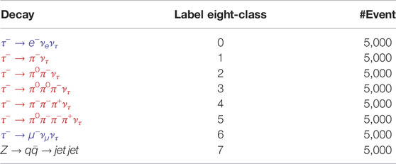
TABLE 1. Decay identification dataset. Leptonic decays in blue and hadronic ones in red.

The process e⁻e⁺ → Z being simulated around the Z pole, the center of mass of the Z boson is still with respect to the interaction point and the two τs or quarks, produced in the decay generate showers in the calorimeter in a back-to-back configuration. This simplified setting allowed us to separate each of the two clusters of any given event by means of simple geometrical clustering methods, without using specific algorithms that take into account models of the physics of the process. Given that in each event there must be two particle showers and that these are in back-to-back configuration, we opted for a simple k-means. Having identified the centroid of each cluster, we extracted the active fibers inside a unit circle around it, $\sqrt{\mathrm{\Delta }{\theta }^2+\mathrm{\Delta }{\varphi }^2}<1$. No fiducial volume has been applied; thus, the part of information of the clusters close to the edges of the calorimeter may have been cut out. We then considered each cluster as an independent data point to be classified.

Performing voxelization or similar operations to regularize the geometric structure of the data would result in the loss of spatial resolution, which would mean hinder a distinctive point of strength of the IDEA calorimeter. Thus, we directly formalized our data as a point cloud. Figure 1 shows few examples of the cluster patterns we obtained.

FIGURE 1

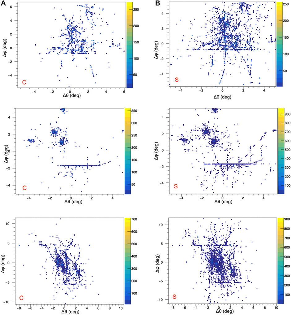
FIGURE 1. Examples from our dataset. Columns represent Cherenkov (A) and scintillation (B) channels; rows represent events. From the top to bottom: QCD jet, τ⁻ → π⁰π⁰π⁻ν_τ, and τ⁻ → π⁰π⁻π⁻π⁺ν_τ.

Given a fiber fired in an event, the following features are collected:

• geometric information: in a first approximation, we used the distance in polar coordinates (Δθ e Δϕ) from the center of the cluster, which leads to a partial distortion of the patterns close to the endcaps of the calorimeter;

• energy information: total number of photo-electrons and total energy released in the fiber;

• fiber type: one-hot encoding of active fiber’s type (Cherenkov or scintillating);

• SiPM electronic information: integral and peak of the signal, time of arrival, time over threshold, and time of peak.

A summary of the available features is reported in Table 2.

TABLE 2

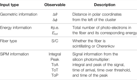
TABLE 2. List of the observables of a fired fiber available in the dataset used in our study.

A nice advantage in using a point cloud representation is that incorporating additional information is straightforward, and it is sufficient to concatenate the additional vectors to the internal representation of each point. Thus, our method can simply be extended to include additional data coming from the calorimeter itself or from other detectors, for e.g., the inner tracker and the muon spectrometer.

2.2 Dynamic Graph CNN

The main property that a model has to ensure when operating on point clouds for classification tasks is permutation invariance, i.e., the output has to be constant regardless of the order in which the inputs are presented to it. In the most recent literature, various architectures can be found that ensure such a property and directly manipulate raw point cloud structured data, for e.g., [29, 34, 38, 41]. Point clouds inherently lack topological information; thus, a model able to recover topology can enrich their representation power. We opted for a dynamic graph convolutional neural network (DGCNN) [38], a graph-based model which explicitly takes advantages of local geometric structure.

The original module introduced in the aforementioned work is named EdgeConv, suitable for CNN-based high-level tasks on point clouds, including classification and segmentation. It is an operation that, while maintaining permutation equivariance, constructs from the point cloud of a local neighborhood graph and applies convolution-like operation on the edges connecting neighboring pair of points, in the spirit of graph neural networks [42, 43].

Given a point cloud X = {x₁, x₂, … , x_N}, where each $x_i\in {\mathbb{R}}^F$, an EdgeConv block first encodes its geometrical structure building a k-nn-directed graph with self-loops, i.e., connections from a vertex to itself (see Figure 2). Then, for each i − th node of the graph, it extracts its edge features e_ij by means of a nonlinear function $h_{\mathrm{\Theta }}:{\mathbb{R}}^F\times {\mathbb{R}}^F\to {\mathbb{R}}^{F^{\prime }}$ with learnable parameters Θ, for e.g., an MLP neural network, in the formula: e_ij = h_Θ(x_i, x_j). Finally, the EdgeConv applies a channel-wise aggregation operation □ on the edge features associated to each point, for e.g., max-pooling or a sum. Thus, the output of the layer is of the form:

$x_i^{\prime }={\square }_{j\in \mathcal{N}\left(x_i\right)}{h}_{\mathrm{\Theta }}\left(x_i,x_j\right).(1)$

In particular, in the original formulation, the operator is defined, channel-wise, as:

$\left\{\begin{array}{c}{e}_{ij}=ReLU\left(\theta \cdot \left(x_j-x_i\right)+\varphi \cdot x_i\right),\hfill \\ x_i^{\prime }=ma{x}_{j\in \mathcal{N}\left(x_i\right)}{e}_{ij}\hfill \end{array}\right..(2)$

FIGURE 2

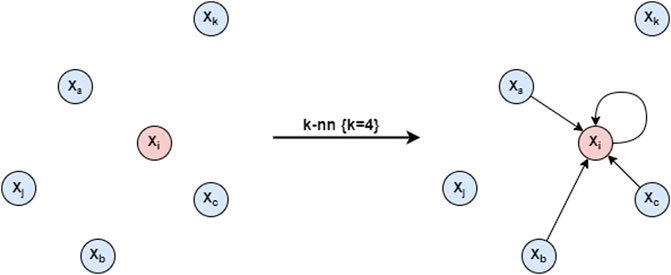
FIGURE 2. In each EdgeConv block, a k-nn graph with self-loops is built from the point cloud, example with k = 4.

Overall, given an F-dimensional point cloud with n points, EdgeConv produces an F′-dimensional point cloud with the same number of points. A basic scheme of the module is depicted in Figure 3.

FIGURE 3

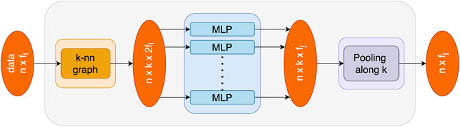
FIGURE 3. Basic EdgeConv block, as introduced in [38].

The Edge block can be integrated into deep learning models to improve their performance. In the original DGCNN article, it is integrated into the basic version of PointNet [34]. Its resulting structure, shown in Figure 4, can be schematized with:

• a hierarchical feature extractor composed by a sequence of EdgeConv layers with skip-connections [20];

• an aggregator (max, avg, or sum) that produces a global feature for the whole point cloud;

• a classifier, implemented in the original article with MLPs.

FIGURE 4

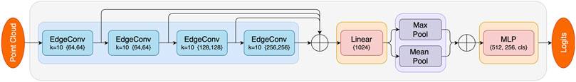
FIGURE 4. DGCNN architecture for tau decay identification.

The characteristic that differentiates DGCNN from other graph-based neural network architectures is that it does not make use of a fixed graph but rather dynamically updates it in each layer of the network. The k-neighborhood of each point may change from layer to layer, and thus proximity in feature space differs from proximity in the input. This leads to non-local diffusion of information throughout the point cloud and makes the receptive field as large as the diameter of the point cloud, while being sparse.

The DGCNN architecture requires a fixed number of points for each point cloud representing the events. The dataset studied in our experiments contains a highly variable number of active fibers per event, ranging from 150 to as much as 4,000. To tackle this problem, as already carried out in [35], the number of fibers considered for each event was fixed to a specific number n, which we treated as an hyperparameter to be tuned. In the case the active fibers were more than n, the ones with the lowest values of signal integral were discarded; if, instead, the number of active fibers was lower than n, a set of zero-valued artificial points is added in order to reach the correct number. We keep track of the possibly present artificial vectors by means of binary masks associated to each cluster. These are used to shift far from zero coordinates of the added vectors in such a way not to introduce artefacts when the k-nn graph is generated and to zero-out their computed features at the output of each EdgeConv block, as shown in Figure 5.

FIGURE 5

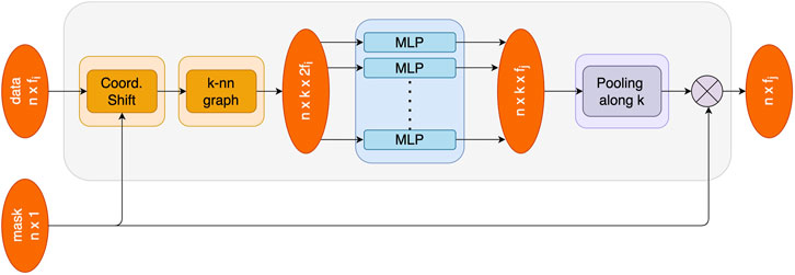
FIGURE 5. EdgeConv block augmented with masks for synthetic datapoints.

2.3 Bayesian Neural Networks

It is not straightforward to extract confidence measures on the predictions of neural networks. In particular, in classification tasks, we should not expect that the last Softmax layer probabilities reflect their ground truth correctness likelihood. It has in fact been showed that, despite the recent improvements in terms of accuracy, most modern neural networks are not well-calibrated [18].

When performing physics experiments, the evaluation of the uncertainty is an integral part of every measurement; a measured value without the corresponding uncertainty only provides partially useful physical information. For example, evaluating the measurement uncertainty is fundamental in scientific research to establish the validity limits of theories. Being able to assign a reliable confidence estimate on a prediction made by a deep learning model is therefore crucial in the context of physics experiments and one viable solution to attain this are Bayesian neural networks.

While in traditional neural networks, deterministic values are inferred for the model parameters in the training phase, these point estimates are replaced by probability distributions in the Bayesian approach. This is carried out extending standard networks with posterior inference, i.e., adding a prior distribution on the model parameters. From a statistician’s point of view, this is equivalent to switching from a maximum likelihood estimation of traditional neural networks (or a maximum a posteriori estimation when regularization is used) to a Bayesian inference approach [26].

This approach allows to measure uncertainty and identify out-of-distribution inputs while regularizing the whole network and preventing overfitting of the training data [17]. Training a BNN can be interpreted as training an infinite ensemble of models with the same structure [44]. An estimate of the uncertainty of the BNN can be obtained by comparing the predictions of multiple sampled model parameterizations: the uncertainty is low when there is agreement among different models, otherwise high.

Among the various approaches to infer the posterior distribution of the model parameters [9, 14, 23, 31], given the complexity of our network, we opted for a variational approach, namely, the Bayes by Backprop algorithm introduced originally in [9].

From our point of view, the advantages of this approach are that:

• the loss is still completely differentiable thanks to the reparameterization trick, thus enabling the use of the backpropagation algorithm;

• the number of parameters only doubles with respect to the corresponding non-Bayesian model, given that each weight w_i is approximated by a normal distribution with the mean μ_i and standard deviation σ_i;

• the training phase is fast, and any deterministic model can be easily extended to its Bayesian counterpart.

Following the Bayes by Backprop approach, we have designed a Bayesian DGCNN that shares essentially the same architecture of the DGCNN but with each weight replaced by a normal distribution described by the mean and the standard deviation as learnable parameters.

3 Results

3.1 Decay Classification

The main task we want to solve is to correctly match single tau clusters reconstructed in the dual-readout calorimeter with the respective decay channel of the tau lepton and distinguishing them from clusters due to QCD jet events. As described in Section 2.1, tau and QCD jets used in this study are produced from Z decays. The classification was performed directly on the raw data collected from the IDEA calorimeter, treating each cluster of each event as an independent point cloud, with each point exhibiting the features listed in Section 2.1.

We balanced our dataset keeping 5,000 clusters for each decay channel, as shown in Table 1. This does not correspond to the true probabilities of each decay type to occur but ensures that our classifier is independent of any prior and bases its estimations only on patterns found in the calorimeter readout signals.

We treated most of the architectural parameters of our network as hyper-parameters to be optimized on the validation set. The resulting architecture consists in a feature extractor of four EdgeConv layers, each composed of two-layered MLPs with the following dimensions: \{64, 64\}, \{64, 64\}, \{128, 128\}, and \{256, 256\}. We composed the aggregator as an MLP of dimension 1024 followed by the parallel max and average pooling blocks. Finally, the classifier was implemented with a two-hidden layered MLP of dimension \{512, 256\} and an eight-class Softmax layer as output, for a total number of parameters in the order of 1.9M, in line with the other SOTA models for point-cloud classification. The complete network architecture is schematized in Figure 4.

As regularization, we introduced batch normalization layers after each EdgeConv and dropout layers before each linear layer in the MLP classifier. Various methods for data augmentation were investigated to improve robustness; a random sparsification of the input turned out to yield best results in terms of generalization, surprisingly enough with a relatively low retention probability (fibers zeroed out with probability ∼0.7). Finally, we applied early stopping on the validation accuracy over a total of 200 epochs, enough to guarantee convergence.

We list here the other optimal parameters and the training setting: learning rate: E-03, optimizer: Adam, step scheduler with γ: 0.5 and milestones: [25, 50, 75], batch size: 64, dropout probability: 0.5, input dimension: 2000, k: 10 (for knn in EdgeConv), pooling: max (in EdgeConv), and activation functions: LeakyReLU with slope 0.1.

An assumed advantage of dual-readout technology is that the patterns generated in the calorimeter would be easily identifiable thanks to the different properties of the fibers that constitute it. To test the informativeness of the patterns and attest the gain in discriminability given by the information about the two different fiber types and as a first benchmark for our model, we trained the DGCNN using as node features the geometric information only, namely, the distances in polar coordinates from the cluster centroid of the fired fibers and the geometric information concatenated with the one-hot encoding of the fiber type; in both cases, no energetic information was provided to the model. We obtain an overall accuracy of 73.7% in the geometric only configuration and of 88.3% when adding the fiber type information; Figure 6 compares the confusion matrices (normalized per row) obtained in these two settings. This result provides a first interesting conclusion: leveraging the differential information provided by the scintillation and Cherenkov fibers of the dual readout calorimeter significantly improves the tau identification performance compared to using geometric information alone. The neural network in fact can efficiently use the information coming from the dual-readout for particle identification and the information about the fiber type results particularly important to discriminate among the hadronic decays (rows 2–6).

FIGURE 6

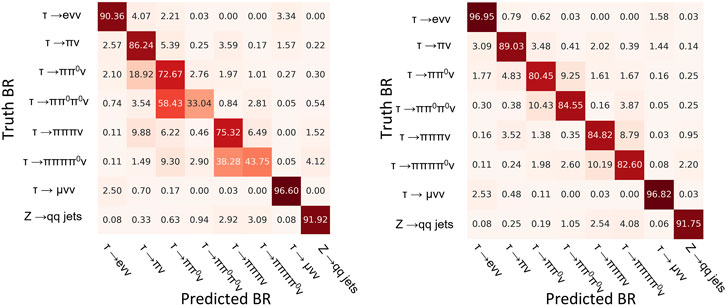
FIGURE 6. Confusion matrices of DGCNN on the test dataset, using geometric only and geometric+fiber type information. Matrices are normalized per row.

We then tested performance improvement that can be achieved by adding as features for each fiber the quantities available from the readout electronic simulation: energy information as the integral and peak of the SiPM signal and temporal information, namely, the time of arrival (ToA), time of peak (ToP), and time over threshold (ToT). We experimented with different configurations, always including the geometrical and fiber type information, to have an estimate of feature importance. The results are summarized in Table 3, and confusion matrices on the test set are reported in Figure 7. The temporal information, more than the energy, seems particularly informative for the model. We speculate that this is due to the fact that temporal information can be interpreted by the model as a proxy measure of the depth in which the particles interact with the calorimeter, adding a third dimension to the absorption patterns. In this particular dataset, produced around the Z pole, the use of energy information could in principle induce in the model a bias over the distribution of the total energy per event. We plotted (Figure 8) such distributions for each decay mode both using the true labels and the labels predicted by our model, and we found no systematic variation between them. Ulterior experiments were performed in a setting with only three classes (leptonic and hadronic tau decays and quark jets), but we found no improvements with respect to the eight-class model performances relative to those decay modes.

TABLE 3

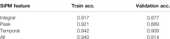
TABLE 3. Train and validation accuracies obtained using SiPM features. In addition to the SiPM features, both coordinates and fiber type information were fed to the model in all experiments.

FIGURE 7

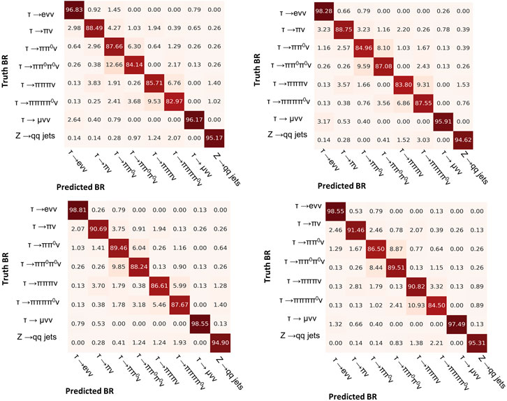
FIGURE 7. Confusion matrices of DGCNN on the test dataset using as features, respectively, in clockwise order from the op left: only integral, only peak, only temporal, or whole SiPM information. In each model, geometric and fiber type information was also used. Matrices are normalized per row.

FIGURE 8

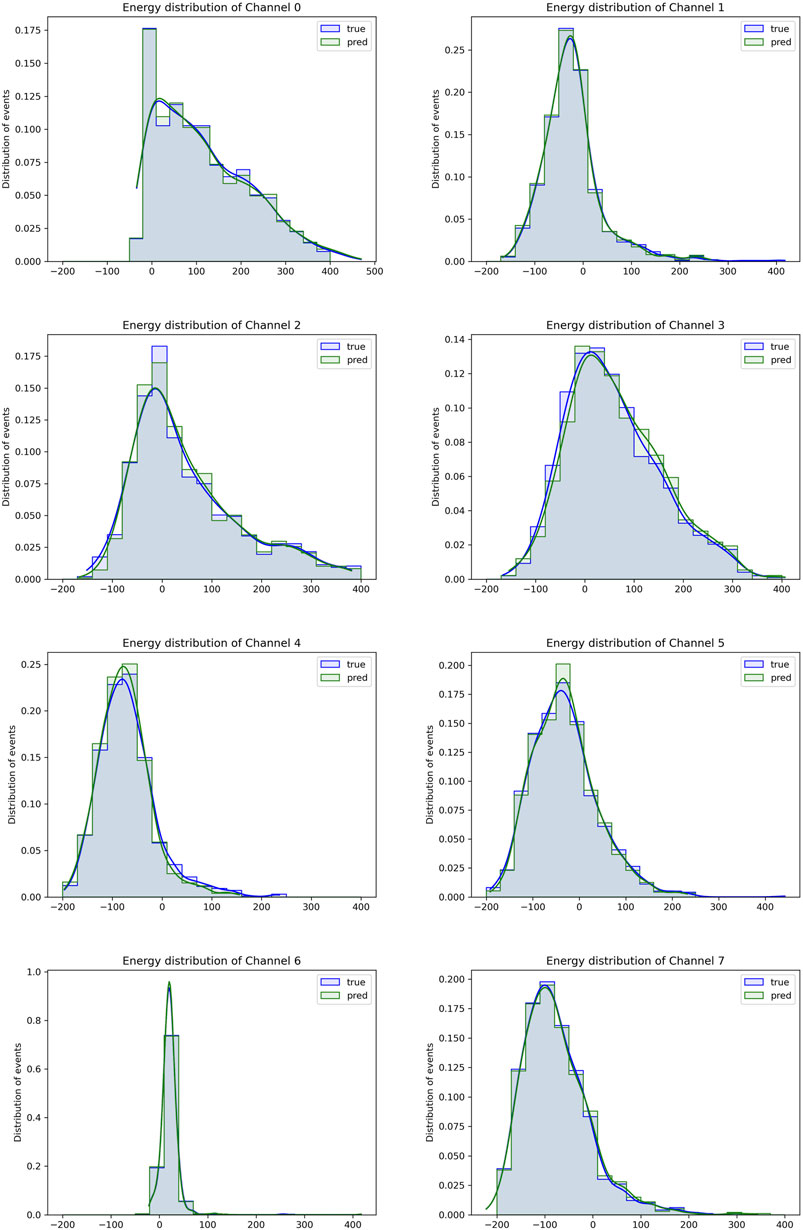
FIGURE 8. Distribution of total energy per event for eight decay channels. Channels are referred to Table 1.

3.2 Uncertainty Estimation With a Bayesian DGCNN

The architecture of our BNN is essentially the same as the model described in Section 3.1, with each weight replaced by a normal distribution defined by the trainable parameters (μ, σ), representing, respectively, the mean and the standard deviation of the distribution, so that the total number of parameters roughly doubles with respect to its deterministic counterpart.

Frequently, when transposing a deterministic network to its Bayesian counterpart, only the weights of the last few layers of the network are treated as distributions, as this simplifies the implementation and the computational complexity of the problem. We found out instead that our model achieved better performance in terms of generalization converting to the Bayesian framework all convolutional and fully connected layers of the model and removing instead all dropout and batch normalization layers. The only other notable difference with the deterministic DGCNN model is the use of scaled exponential linear units (SELUs) as an activation function, known to induce self-normalizing properties [27] in the neural networks improving stability and robustness.

We used the whole information as input features from the calorimeter simulation, being the configuration, which performed best in the deterministic case. Even if not strictly necessary to compute the KL divergence, the values of the parameters are sampled multiple times at each training step, to give more stability to the optimization process. Using three samples in each iteration provided a good trade-off between memory usage and performances.

In Figure 9, for the four most challenging classes of decay, we show improvements in terms of ROC curves and AUC of the Bayesian model over the deterministic one. Table 4 shows the accuracies reached in the test phase for different number of samplings considering all the events and for different minimum confidence thresholds on the final prediction. We do not find much improvement in terms of overall accuracy and confidence of the model when using more than 10 samples at test time. In Figure 10, we compare confusion matrices on the test set applying no threshold or a 0.7 threshold on the minimum confidence of the prediction.

FIGURE 9

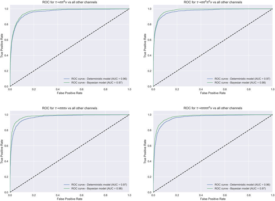
FIGURE 9. ROC curves of the Bayesian DGCNN and point-estimate DGCNN for four classes of decay.

TABLE 4

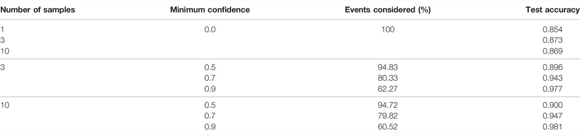
TABLE 4. Bayesian DGCNN test accuracies by varying number of samples of network parameters and minimum confidence in the classification prediction.

FIGURE 10

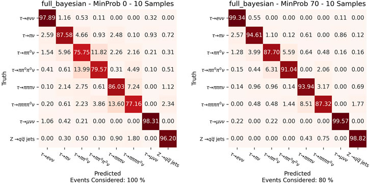
FIGURE 10. Confusion matrices of the Bayesian DGCNN with 10 samples for each prediction without a threshold on minimum confidence and with a minimum confidence of 0.7. In the bottom, it is indicated the rate of events considered.

4 Discussion

In this study, we propose a new technique based on the use of deep neural networks for the identification of tau lepton decays and show its performance when applied to the IDEA dual-readout calorimeter concept proposed for the future FCC-ee electron–positron collider. We have implemented a dynamic graph CNN architecture that takes in input only the raw information from the readout electronic of the calorimeter and leveraging the high granularity, and the different patterns produced by the dual readout is able to predict with excellent performance the specific tau lepton decay, discriminating also taus against signals produced by QCD jet events. An average accuracy of 91% in classifying different tau decays is obtained by using geometrical, energy, and time information from the calorimeter’s fibers, while the accuracy for the specific decay modes ranges from 99% for the leptonic decays of the tau to 85–90% for the hadronic modes. The model is also able to discriminate with high-accuracy ($>$95%) tau decays from jets from QCD. Even by using as input of the neural network only the information relative to the geometry and the type, scintillating or Cherenkov, of the firing fibers, the model is able to achieve average accuracies between 80 and 97% depending on the decay mode. The proposed algorithm is very flexible and can be easily extended in terms of additional tasks and additional input features, as for example, information from other detector systems. The ongoing work focuses on extending the capabilities of the algorithm by including information from other detector subsystem (inner tracking and muon spectrometer) and in identifying the individual contributions from the neutral and charged particles inside the tau and QCD jet clusters, to further improve the particle identification and particle flow reconstruction.

Data Availability Statement

The datasets and the original code used for this study are available on request by contacting the corresponding authors.

Author Contributions

SG proposed the original idea, coordinated the work, prepared the dataset, and performed the initial proof of concept implementation; LT implemented and trained the DGCNN model for the classification task and contributed to the data analysis; MD implemented the Bayes DGCNN model and contributed to the data analysis. All authors wrote the manuscript, contributed to the manuscript, and approved the submitted version.

Funding

This work was partially funded by the Istituto Nazionale di Fisica Nucleare, Sezione di Roma.

Conflict of Interest

The authors declare that the research was conducted in the absence of any commercial or financial relationships that could be construed as a potential conflict of interest.

Publisher’s Note

All claims expressed in this article are solely those of the authors and do not necessarily represent those of their affiliated organizations, or those of the publisher, the editors, and the reviewers. Any product that may be evaluated in this article, or claim that may be made by its manufacturer, is not guaranteed or endorsed by the publisher.

Acknowledgments

We are greatly indebted to the IDEA dual-readout calorimeter concept group, especially the University and INFN Pavia and the University of Insubria groups, for the fundamental help in providing the simulated event samples used to train and test the algorithms and in understanding the specific features of the dual-readout calorimeter.

References

1. Abada A, Abbrescia M, AbdusSalam SS, Abdyukhanov I, Fernandez JA, Abramov A, et al. Fcc-ee: the Lepton Collider. Eur Phys J Spec Top (2019) 228:261–623. doi:10.1140/epjst/e2019-900045-4

CrossRef Full Text | Google Scholar

2. Antonello M, Caccia M, Ferrari R, Gaudio G, Pezzotti L, Polesello G, et al. Expected Performance of the Idea Dual-Readout Fully Projective Fiber Calorimeter. J Inst (2020) 15:C06015. doi:10.1088/1748-0221/15/06/c06015

CrossRef Full Text | Google Scholar

3.ATLAS collaboration. Observation of a New Particle in the Search for the Standard Model Higgs Boson with the Atlas Detector at the Lhc. Phys Lett B (2012) 716:1–29. doi:10.1016/j.physletb.2012.08.020

CrossRef Full Text | Google Scholar

4. Aad G, Abbott B, Abdallah J, Abdel Khalek S, Abdinov O, Aben R, et al. Identification and Energy Calibration of Hadronically Decaying Tau Leptons with the Atlas experiment in Pp Collisions at $\sqrt{s}$=8 Tev. Eur Phys J (20152015) C75:303. doi:10.1140/epjc/s10052-015-3500-z

CrossRef Full Text | Google Scholar

5. Aad G, Abbott B, Abdallah J, Abdinov O, Aben R, AbouZeid OS, et al. Measurements of the Higgs Boson Production and Decay Rates and Coupling Strengths Using Pp Collision Data at $\sqrt{s}$=7 and 8 Tev in the Atlas experiment. The Eur Phys J C (2016) 76:1–51. doi:10.1140/epjc/s10052-015-3769-y

CrossRef Full Text | Google Scholar

6. Aaboud M, Aad G, Abbott B, Abdinov O, Abeloos B, Abidi SH, et al. Measurement of τ Polarisation in Z/γ* → ττ Decays in Proton–Proton Collisions at $\sqrt{s}=8$ Tev with the Atlas Detector. Eur Phys J C (2018) 78:163. doi:10.1140/epjc/s10052-018-5619-1

PubMed Abstract | CrossRef Full Text | Google Scholar

7. Aubert B, Karyotakis Y, Lees J, Poireau V, Prencipe E, Prudent X, et al. Searches for lepton flavor violation in the decays τ^± → e^±γ and τ^± → μ^±γ. Phys Rev Lett (2010) 104:021802. doi:10.1103/PhysRevLett.104.021802

PubMed Abstract | CrossRef Full Text | Google Scholar

8. Benedikt M, Mertens V, Zimmermann F, Cerutti F, Otto T, Poole J, et al. Fcc-ee: The Lepton Collider: Future Circular Collider Conceptual Design Report Volume 2. Eur Phys J Spec Top (2018) 228:261–623. doi:10.1140/epjst/e2019-900045-4

CrossRef Full Text | Google Scholar

9. Blundell C, Cornebise J, Kavukcuoglu K, Wierstra D. Weight Uncertainty in Neural Network. In: International Conference on Machine Learning (PMLR) (2015). p. 1613–22.

Google Scholar

10.CMS Collaboration (2015). Reconstruction and Identification of Tau Lepton Decays to Hadrons and Tau Neutrino at Cms. arXiv preprint arXiv:1510.07488. doi:10.1088/1748-0221/13/10/P10005

CrossRef Full Text | Google Scholar

11.CMS collaboration. Performance of Reconstruction and Identification of τ Leptons Decaying to Hadrons and ντ in Pp Collisions at $\sqrt{s}$= 13 Tev. JINST (2018) 13:P10005.

Google Scholar

12. Dam M. Tau-lepton physics at the fcc-ee circular e⁺e⁻ collider. Sci Post Phys Proc (2019) 41. doi:10.21468/SciPostPhysProc.1.041

CrossRef Full Text | Google Scholar

13. Elagin A, Safonov A. Likelihood-based Particle Flow Algorithm at Cdf for Accurate Energy Measurement and Identification of Hadronically Decaying Tau Leptons. In: Proceedings of 13th International Workshop on Advanced Computing and Analysis Techniques in Physics Research — PoS(ACAT2010), 093 (2010). doi:10.22323/1.093.0046

CrossRef Full Text | Google Scholar

14. Gal Y, Ghahramani Z. Dropout as a Bayesian Approximation: Representing Model Uncertainty in Deep Learning. In: international conference on machine learning (PMLR) (2016). p. 1050–9.

Google Scholar

15. Galea C. Tau Identification at D0. Acta Phys.Polon. (2007) B38:769–78.

Google Scholar

16.GEANT Collaboration Agostinelli S, Allison J, Amako K, Apostolakis J, Araujo H, et al. Geant4–a Simulation Toolkit. Nucl Instrum Meth A (2003) 506:250–303. doi:10.1016/S0168-9002(03)01368-8

CrossRef Full Text | Google Scholar

17. Goan E, Fookes C. Bayesian Neural Networks: An Introduction and Survey. In: Case Studies in Applied Bayesian Data Science. Springer (2020). p. 45–87. doi:10.1007/978-3-030-42553-1_3

CrossRef Full Text | Google Scholar

18. Guo C, Pleiss G, Sun Y, Weinberger KQ. On Calibration of Modern Neural Networks. In: International Conference on Machine Learning (PMLR) (2017). p. 1321–30.

Google Scholar

19. Hayasaka K, Inami K, Miyazaki Y, Arinstein K, Aulchenko V, Aushev T, et al. Search for Lepton-Flavor-Violating τ Decays into Three Leptons with 719 Million Produced τ+ τ- Pairs. Phys Lett B (2010) 687:139–43. doi:10.1016/j.physletb.2010.03.037

CrossRef Full Text | Google Scholar

20. He K, Zhang X, Ren S, Sun J. Deep Residual Learning for Image Recognition. In: Proceedings of the IEEE conference on computer vision and pattern recognition (2016). p. 770–8. doi:10.1109/cvpr.2016.90

CrossRef Full Text | Google Scholar

21. Heister et al. A. Measurement of the Tau Polarisation at Lep. Eur Phys J C (2001) 20:401–30. doi:10.1007/s100520100689

CrossRef Full Text | Google Scholar

22. Heldmann M, Cavalli D. An Improved Tau-Identification for the ATLAS experiment. Tech Rep (2005).

Google Scholar

23. Hernández-Lobato JM, Adams R. Probabilistic Backpropagation for Scalable Learning of Bayesian Neural Networks. In: International conference on machine learning (PMLR) (2015). p. 1861–9.

Google Scholar

24.High Luminosity LHC Project (2021). The Hl-Lhc Project. [Online; accessed 1-February-2022]

Google Scholar

25. Innocente V, Wang YF, Zhang ZP. Identification of Tau Decays Using a Neural Network. Nucl Instr Methods Phys Res Section A: Acc Spectrometers, Detectors Associated Equipment (1992) 323:647–55. doi:10.1016/0168-9002(92)90011-r

CrossRef Full Text | Google Scholar

26. Jospin LV, Buntine W, Boussaid F, Laga H, Bennamoun M (2020). Hands-on Bayesian Neural Networks–A Tutorial for Deep Learning Users. arXiv preprint arXiv:2007.06823

Google Scholar

27. Klambauer G, Unterthiner T, Mayr A, Hochreiter S. Self-normalizing Neural Networks. In: Proceedings of the 31st international conference on neural information processing systems (2017). p. 972–81.

Google Scholar

28. Levy S (2005). Tau Identification at the Tevatron. Tech. rep., Fermi National Accelerator Lab.(FNAL), Batavia, IL (United States). doi:10.1007/978-3-540-32841-4_20

CrossRef Full Text | Google Scholar

29. Li Y, Bu R, Sun M, Wu W, Di X, Chen B. Pointcnn: Convolution on X-Transformed Points. Adv Neural Inf Process Syst (2018) 31. doi:10.48550/arXiv.1801.07791

CrossRef Full Text | Google Scholar

30. Lindfeld L. Tau Leptons at Hera. Nucl Phys B - Proc Supplements (2005) 144:315–22. doi:10.1016/j.nuclphysbps.2005.02.042

CrossRef Full Text | Google Scholar

31. Neal RM, Mcmc Using Hamiltonian Dynamics. Handbook of markov chain monte carlo (2011) 2:2. doi:10.1201/b10905-6

CrossRef Full Text | Google Scholar

32. Perl ML. The Tau Lepton. Rep Prog Phys (1992) 55:653–722. doi:10.1088/0034-4885/55/6/001

CrossRef Full Text | Google Scholar

33. Proserpio E, Santoro R. SimSiPM: A Library for SiPM Simulation. Como, Italy (2021).

Google Scholar

34. Qi CR, Su H, Mo K, Guibas LJ. Pointnet: Deep Learning on point Sets for 3d Classification and Segmentation. In: Proceedings of the IEEE conference on computer vision and pattern recognition (2017). p. 652–60.

Google Scholar

35. Qu H, Gouskos L. Jet Tagging via Particle Clouds. Phys Rev D (2020) 101:056019. doi:10.1103/physrevd.101.056019

CrossRef Full Text | Google Scholar

36. Safonov AN. Physics with Taus at Cdf. Nucl Phys B - Proc Supplements (2005) 144:323–32. doi:10.1016/j.nuclphysbps.2005.02.043

CrossRef Full Text | Google Scholar

37. Sjöstrand T, Mrenna S, Skands P. A Brief Introduction to Pythia 8.1. Comput Phys Commun (2008) 178:852–67. doi:10.1016/j.cpc.2008.01.036

CrossRef Full Text | Google Scholar

38. Wang Y, Sun Y, Liu Z, Sarma SE, Bronstein MM, Solomon JM. Dynamic Graph Cnn for Learning on point Clouds. ACM Trans Graph (2019) 38:1–12. doi:10.1145/3326362

CrossRef Full Text | Google Scholar

39. Wigmans R. The DREAM Project-Results and Plans. Nucl Instr Methods Phys Res Section A: Acc Spectrometers, Detectors Associated Equipment (2007) 572:215–7. doi:10.1016/j.nima.2006.10.211

CrossRef Full Text | Google Scholar

40. Wigmans R, New Results from the Rd52 Project. Nucl Instr Methods Phys Res Section A: Acc Spectrometers, Detectors Associated Equipment (2016) 824:721–5. doi:10.1016/j.nima.2015.09.069

CrossRef Full Text | Google Scholar

41. Wu W, Qi Z, Fuxin L. Pointconv: Deep Convolutional Networks on 3d point Clouds. In: Proceedings of the IEEE/CVF Conference on Computer Vision and Pattern Recognition (2019). p. 9621–30. doi:10.1109/cvpr.2019.00985

CrossRef Full Text | Google Scholar

42. Wu Z, Pan S, Chen F, Long G, Zhang C, Yu PS. A Comprehensive Survey on Graph Neural Networks. IEEE Trans Neural Netw Learn Syst (2020) 32:4–24. doi:10.1109/TNNLS.2020.2978386

PubMed Abstract | CrossRef Full Text | Google Scholar

43. Zhou J, Cui G, Hu S, Zhang Z, Yang C, Liu Z, et al. Graph Neural Networks: A Review of Methods and Applications. AI Open (2020) 1:57–81. doi:10.1016/j.aiopen.2021.01.001

CrossRef Full Text | Google Scholar

44. Zhou Z-H. Ensemble Methods: Foundations and Algorithms. New York, NY: CRC Press (2012).

Google Scholar