Classifying Beers With Memristor Neural Network Algorithm in a Portable Electronic Nose System

Quality control and counterfeit product detection have become exceedingly important due to the vertical market of beers in the global economy. China is the largest producer of beer globally and has a massive problem with counterfeit alcoholic beverages. In this research, a modular electronic nose system with 4 MOS gas sensors was designed for collecting the models from four different brands of Chinese beers. A sample delivery subsystem was fabricated to inject and clean the samples. A software-based data acquisition subsystem was programmed to record the time-dependent chemical responses in 28 different models. A back-propagation neural network based on a memristor was proposed to classify the quality of the beers. Data collected from the electronic nose system were then used to train, validate, and test the created memristor back-propagation neural network model. Over 70 tests with changes in the setup parameters, feature extraction methods, and neural network parameters were performed to analyze the classification performance of the electronic nose hardware and neural network. Samples collected from 28 experiments showed a deviation of 9% from the mean value. The memristor back-propagation network was able to classify four brands of Chinese beers, with 88.3% of classification accuracy. Because the memristor neural network algorithm is easy to fabricate in hardware, it is reasonable to design an instrument with low cost and high accuracy in the near future.

1 Introduction

Food quality control is becoming exceedingly popular due to the massive quantities of products in today’s world. But the monitoring of food quality has become more critical with the governments’ regulations and improvements in sensor technology. In the research field, monitoring system design, classification methods, or algorithms have been proved to be effective ways to enhance the accuracy of food detection.

Using an electronic nose to detect the odor of food or beverage, instead of a human nose, was first proposed in 1982. At present, the electronic nose is still an essential way of detecting food quality for different applications. In the monitoring system design, M. Falasconi [1] gave in detail about using electronic nose microbiology for detecting food product quality control in 2012. Gliszczyńska-Świgło [2] reviewed the electronic nose as a tool for monitoring the authenticity of food in 2017. Wojnowski [3] proposed a portable electronic nose based on electrochemical sensors for food quality assessment in 2017. Eusebio [4] published the definition of minimum performance requirements for environmental odor monitoring in electronic nose testing procedures in 2017. For improving the accuracy, Liu [5] researched a drift compensation for electronic noses by semi-supervised domain adaption. Vergara [6] put a chemical gas sensor drift compensation using classifier ensembles. Zhang [7] explained domain adaptation extreme learning machines for drift compensation in e-nose system in 2015. Another Zhang [8] used a chaotic time series prediction of the e-nose sensor drift in the embedded phase space in 2013. In the research objects, tea [9] and wine [10] have been used to monitor their quality. For algorithms, Zhang [11] listed all the methods: SVM, BPA, neural network, and so on, in his book e-Nose Algorithms and Challenges in 2018. Qi [12]designed a portable electronic nose to classify the real–fake detection of Chinese liquors in 2017. Pádua [13] proposed a new design of a scalable and easy-to-use EN system to detect volatile organic compounds from exhaled breath in 2018. The aforementioned articles only proposed monitoring the quality of one type of product as it is difficult to design a universal electronic nose to monitor the quality of multiple products due to inherent limitations of sensor technology.

The memristor is a new emerging technology, which has been developed in the past decade. Li, C.L [14], and Ma [15] focused on how to design and fabricate the memristor circuit. Li, C.L. [16], Li, X.J [17], and Gao [18, 19] used the memristor algorithm to encrypt images. In the past few years, hybrid algorithms based on the memristor and different neural networks were proposed in [20–23].

In this study, a new portable modular design of an electronic nose was proposed to classify four different brands of Chinese beers based on the MOS sensor array and the memristor back-propagation neural network algorithm. After simulation in MATLAB, the system and the algorithm were efficient with higher accuracy in classifying the assigned beers.

2 System Setup and Experimental Procedure

2.1 Sample Delivery Subsystem

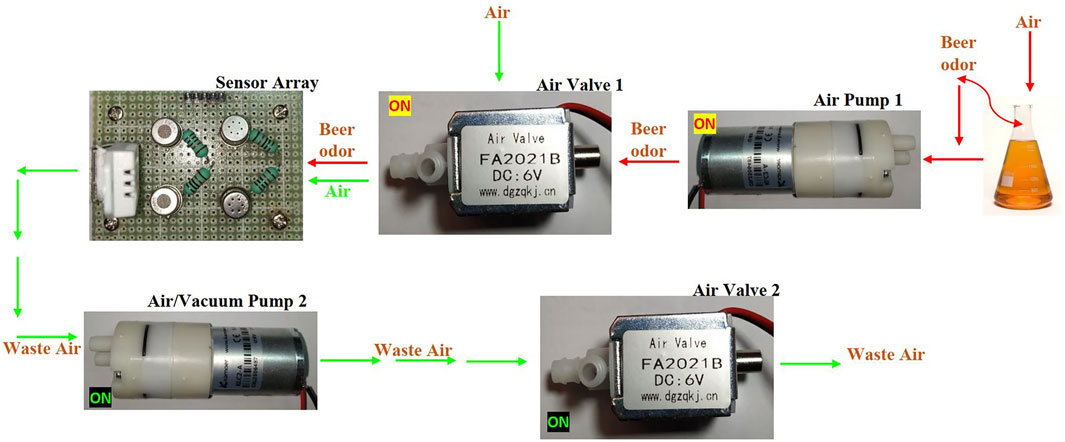
The section consisted of air pumps and air valves with a sophisticated control setup, which diluted the aroma of the beer sample with air in an accurate ratio and delivered it to the gas detection module. The sample delivery system consisted of a sensor array, two solenoid air valves, and two air/vacuum pumps, as shown in Figure 1. During the experiment, in the injection mode (red), solenoid air valve 1 and air pump 1 were turned on. The beer odor sample was then drawn into the sensor chamber using air pump 1 connected to the solenoid air valve 1. In cleaning mode (green), air pump 2 and solenoid air valve 2 were turned on to clean the sensor chamber for the next sample. Air pump 2, working as a vacuum pump, is connected to the sample chamber with pipes to remove odor from it.

FIGURE 1

FIGURE 1. Working modes of sample delivery system.

The sample delivery system was kept inside the EN housing, separated from the gas detection module and the sample chamber. It was connected to the gas detection module and sample chamber through pipes and routings.

2.2 Data Acquisition Subsystem

The gas detection module consists of 4 cross-sensitive MOS sensors (tgs2600, tgs2602, tgs2611, and tgs2620), which detect the mixture of gases present in the aroma. The data acquisition system then collected the response of the gas detection module in real time and stored the time-stamped data. Finally, the memristor back-propagation neural network model was trained to perform pattern recognition based on the response from the gas detection module.

After the hardware design was completed, a working prototype of the electronic nose was able to switch the sample delivery system and convert the sensor response into digital signals. Now, these data were stored for further analysis.

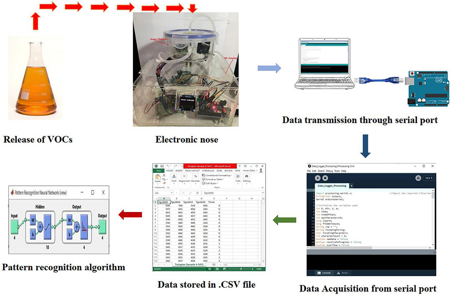
During the testing stage, sensors in the gas detection module were measuring the odor and sending the analog signals to an Arduino microcontroller. A microcontroller ADC converted these analog signals into digital signals and displayed them on its serial port. Processing software was then used to process and store the data in a CSV file. Serial communication was used to deliver data between the microcontroller and PC. The block diagram of data acquisition subsystem is shown in Figure 2.

FIGURE 2

FIGURE 2. Block diagram of data acquisition subsystem.

2.3 Set Experiment Parameters

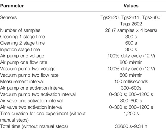
After numerous tests, measurements were taken with the following values of adjustable parameters of the electronic nose (Table 1). Four brands of Chinese beer were bought from different supermarkets. Overall, seven sample bottles of each brand of beer were collected this way for the diversity of samples. Each beer sample was then taken to collect the sensor response curve. The total number of pieces was 28. To ensure uniformity, 50 ml of beer was taken from each sample bottle and poured into the sample chamber. All the experiments for data collection of beer samples were performed within one week, so the sensor array was preheated only once before starting the experiments. All sensors were heated for 48 h to ensure stable sensor characteristics.

TABLE 1

TABLE 1. Set experiment parameters.

2.4 Experiment Procedure

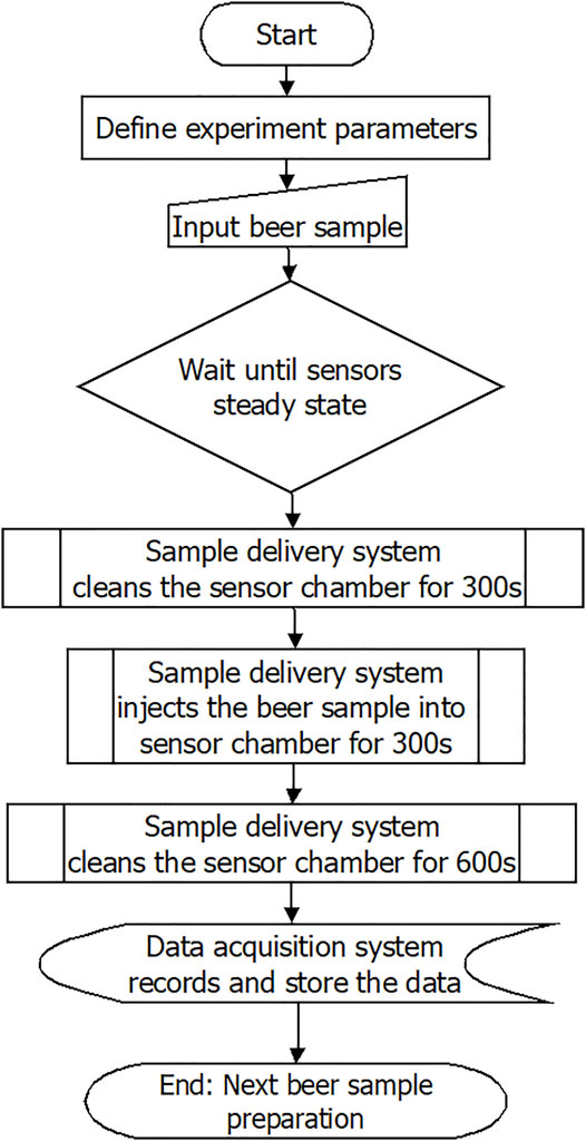
All steps in the system were automated. Only sample preparation was manual. The steps to record one sample were as follows: After defining the experiment parameters, wait until a steady state, then prepare the sample in the sample chamber, turn on the electronic nose, and the system will start. Next, in cleaning stage 1, the sample delivery system activated the air pumps and solenoid air valves to clean the sensor chamber for 300 s. Third, injection stage: the sample delivery system started the air pumps and solenoid air valves to deliver the beer sample odor from sample chamber to sensor chamber for 300 s. Fourth, cleaning stage 2: sample delivery system activated the air pumps and solenoid air valves to clean the sensor chamber for 600 s. During this whole procedure, the data acquisition system records the data and saves it as a CSV file. Finally, clean and wash the sample chamber for subsequent measurement. The flowchart is shown in Figure 3.

FIGURE 3

FIGURE 3. Flowchart of the experiment procedure.

2.3 Memristor Neural Network Design

To classify the different odors of Chinese beers, MATLAB was used to create and ultimately organize the data. Following steps were followed to develop a neural network model, and this neural network was then used to test the input data and classify it according to the recognized patterns in it.

First, four sensors (tgs2600, tgs2602, tgs2611, and tgs2620) were used to record the odor in the sample, so the number of input was defined as 4. The number of outputs was also 4 as four brands of Chinese beers were being used for the classification.

Then, values were initialized. Starting weight values were set for synapses connecting each node. Here random discounts were applied. Next, the middle hidden layer was calculated, four weights from each of the nodes in the input layer were indexed, and four weights from each remote layer node to the output layer were set. Summing up the input values I[n] multiplied by their consequences from the synapses and adding a node threshold value (T) resulted in the consequences from the input layer to the middle hidden layer, which was denoted by I_to_M_weight[i] [24].

$M\left[i\right]=\left({\displaystyle \sum }_1^{n}I\left[n\right]\ast I\_to\_M\_weight\left[i\right]\right)+M\left[i\right]+T(1)$

M[i] was limited between 0 and 1 when adjusted with a sigmoid logistic function.

$M\left[i\right]=\frac{1}{1+e^{-M\left[i\right]}}(2)$

After calculating the hidden layer nodes, constrained values were used to calculate the output layer. Here, the inputs were the middle layer node values, and the outputs were the nodes in the output layer.

$O\left[i\right]=\left({\displaystyle \sum }_1^{n}M\left[n\right]\ast M\_to\_O\_weight\left[i\right]\right)+O\left[i\right]+T(3)$

O[i] was also limited between 0 and 1 when it was adjusted with a sigmoid logistic function.

$O\left[i\right]=\frac{1}{1+e^{-O\left[i\right]}}(4)$

When training began, due to the inherent randomness created during the initialization, the output error $err\left[i\right]$ equaled subtracting the correct value $actual\left[i\right]$ from the output value $O\left[i\right]$ and taking the absolute value.

$err\left[i\right]=abs\left(actual\left[i\right]-O\left[i\right]\right)(5)$

The hidden layer weight values were updated by adding the error between the output and the middle to output weight.

$M\_weight\left[i\right]={\displaystyle \sum }_1^{n}M\_weight\left[i\right]+\left(err\left[n\right]\ast M\_to\_O\_weight[i,n]\right)(6)$

Here, $M\_weight\left[i\right]$ was used to calculate the error at the middle hidden layer. $M\_err\left[i\right]$ was used to reevaluate the input to middleweights.

$M\_err\left[i\right]=M\left[i\right]\ast \left(i-M\left[i\right]\right)\ast M\_weight\left[i\right](7)$

Then, the weights between the middle and output layers could be updated. Here, a learning rate between 0 and 1 was used to balance the degree for each epoch. Due to oscillating the output accuracy, a momentum rate was added to change from previous epochs. The learning rate was set as the following equation:

$M\_to\_O\_weight[a,b]=M\_O\_weight\left[a,b\right]+(learning rate\ast M\left[a\right]\ast err\left[b\right])(8)$

The momentum was in the following equation:

$M\_to\_O\_weight[a,b]=M\_O\_weight\left[a,b\right]+(momentum rate\ast last M\_to\_O\_weight[a,b])(9)$

Now, the weights between the input layer and middle layer were updated based on the error in the middle layer:

$I\_to\_M\_weight[a,b]=I\_to\_M\_weight\left[a,b\right]+(learning rate\ast I\left[a\right]\ast M\_err\left[b\right])(10)$

where a was from 1 to the number of input nodes and b was from 1 to the number of hidden nodes.

Finally, the threshold constants were updated from the error in each layer and the learning rate.

$M\_threshold\left[i\right]=M\_threshold\left[i\right]+(learningrate\ast M\_err\left[i\right])(11)$

$O\_threshold\left[i\right]=M\_threshold\left[i\right]+(learningrate\ast err\left[i\right])(12)$

3 Simulation and Results Analysis

3.1 Set Learning Rate

Collected data were fed into our created neural network model. A new memristor scaled conjugate gradient back-propagation was designed to classify collected samples. The memristor back-propagating neural network used a momentum rate of 0.9 and a floating learning rate that began training at 0.4. As the average training error of the network decreased, the learning rate decreased. The network started with a higher learning and momentum rate to avoid the system becoming stuck in a local minimum or local maximum. As the average training error lowered, the learning rate decreased to try to fine-tune the parameters of the system. The change in the learning rate to the average training error is listed in Table 2.

TABLE 2

TABLE 2. Learning rate adjustment.

3.2 Set Numbers of Hidden Neurons

Multiple sets of hidden neurons were tested, and their effects on classification were analyzed. In this analysis, the number of HNs was changed in the neural network model, and the network was trained and tested each time with a different number of HNs. At the end of each training and testing, confusion matrixes were stored. Overall, 10, 1,000, 2000, 3,000, 4,000, and 5,000 HNs were changed in the NN model, and the results are shown in Table 3. Totally, 10 HNs reported the lowest classification accuracy in the confusion matrix, and 5,000 HNs reported the highest overall accuracy. The effect of the number of HNs was also directly related to the individual classification accuracy of each beer. Each beer classification rate was calculated as average. The highest overall accuracy of 88.3% was achieved with 5,000 hidden neurons. During this analysis, all other parameters in this neural network model remained the same.

TABLE 3

TABLE 3. Comparison of classification accuracy with change in number of hidden neurons.

3.3 Type of Feature Extraction Method

Two types of feature extraction were done on data and then fed into our neural network model. The first type of feature extraction was based on the original response curve. In this type of feature extraction, features were extracted from the whole curve. The whole curve included the baseline response and sensor response to the beer sample. Rather than taking full value features of the response curve, data from the entire curve were stored and given as input to the NN model. In the second type, feature extraction was based on the rising curve. In this type of feature extraction, the only rising curve was taken as the feature curve where features were extracted from only the rising curve data.

Changes in the feature extraction method drastically affected the overall classification accuracy of beer samples. When the neural network was trained based on the features from the original response curve, it reported a maximum accuracy of 87.8% with 4,000 hidden neurons. But the NN model reported only 79.6% classification accuracy with 4,000 hidden neurons when the NN model was trained using features extracted from the rising curve. Accuracy comparison of rising and whole curves with 1,000 and 4,000 hidden neurons is shown in Figure 4. Average accuracies for individual beers were also reported to be decreased.

FIGURE 4

FIGURE 4. Confusion matrices with rising and whole curve along with 1,000 and 4,000 hidden neurons.

3.4 Validation and Test Data

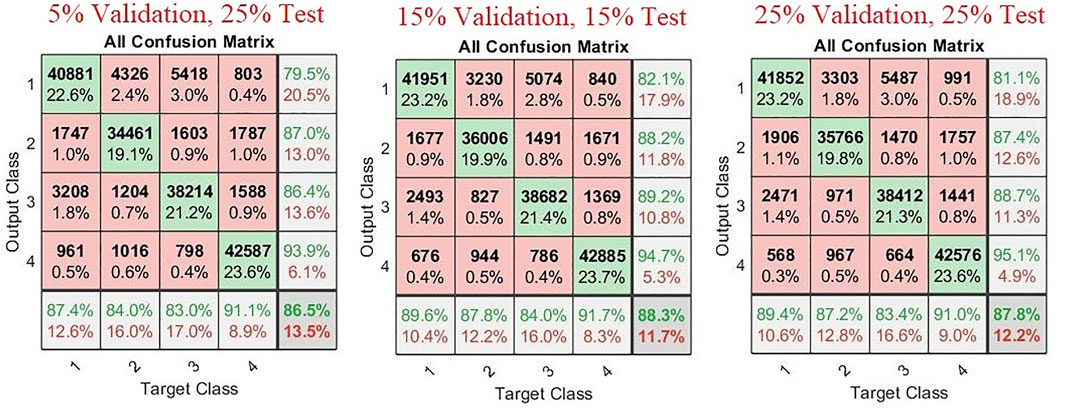
To perform classification with a neural network, it has to be trained, validated, and then tested to give accurate predictions. To check the effect of the amount of validation data and test data on the classification accuracy of our trained model, these parameters were changed and analyzed. Training data of created neural network were kept at 70% of total data during two variations, and it was reduced to 50% of total data in the third variation. Remaining 30% data were then divided into validation and test data of multiple variations (15% validation data, 15% test data), (5% validation data, 25% test data), and (25% validation data, 25% test data).

During this analysis, all the other parameters in the system were kept constant. Hidden neurons during this analysis were maintained at 5,000. Features extracted from the whole response curve were used as feature extraction types. Study (Figure 5) showed that the maximum classification accuracy of 88.3% was achieved with (15% validation data and 15% test data), while (25% validation data, 25% test data) attained an accuracy of 87.8%. Parameters of (5% validation data, 25% test data) performed the worst and showed an accuracy of only 86.5%.

FIGURE 5

FIGURE 5. Confusion matrices with different percentages of validation data and test data.

3.5 Doubling the Amount of Data

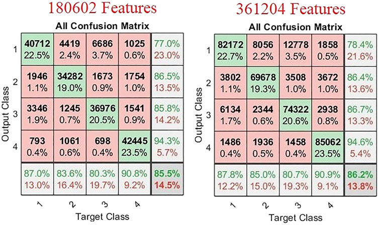
The number of samples recorded with our working prototype was 28, which were divided into seven samples of 4 different brands of Chinese beers. The number of features extracted from these 28 samples was 180602. These features were then used to train, validate, and test our neural network. Components were randomly selected, and the amount of data for training, validation, and testing was also randomly selected. Idea was presented to investigate if doubling the amount of data would increase its accuracy or not. Due to time constraints, data collection was not possible. We adopted the method of duplicating features. In this technique, we extracted features from our original data, which were 180602, and repeated them. The amount of features after duplication was 361204. These repeated features were then used for the training, validation, and testing of neural networks. In this analysis, the number of hidden neurons was taken as 1,000, and the whole response curve was used for feature extraction. In this study, 70% of all data were used as training data, and the remaining data were used for validation and training. Out of 30% remaining data, 15% were used for validation and 15% for testing the trained NN model. By doubling the number of features, a 0.7% overall increase in classification accuracy of the trained neural network was reported (Figure 6). But it also doubled the processing time. The time to train the neural network also significantly increased as the amount of data increased.

FIGURE 6

FIGURE 6. Confusion matrices of the neural network model with different amounts of features.

3.6 Classification of Chinese Beers

To perform the classification of Chinese beers, multiple analyses were done on the different parameters of the neural network. The trained neural network reported a maximum accuracy of 88.3% in Section 3.4. In this neural network model, 5,000 hidden layers were taken. Feature extraction was based on the original response curve, which means the features included the steady-state and the transient response of each sample. Total samples were 28, and the number of components extracted was 180602. Again 70% of the complete data were taken as training data. Training of the NN lasted 4 h, which was done on a laboratory computer. Of the remaining data, 15% were used for validation, and another 15% were used for testing the trained NN model. All the features used in training, validation, and testing were randomly selected. The confusion matrix of this NN model is shown in Figure 7. The receiver operating characteristic curve (ROC) of this trained neural network is established in Figure 8.

FIGURE 7

FIGURE 7. Confusion matrix with maximum classification accuracy.

FIGURE 8

FIGURE 8. Receiver operating characteristic curve with maximum classification accuracy.

The ROC curve of the trained neural network also demonstrated the accuracy of the trained NN model during the classification; it stayed true to the proper positive rate curve. During training, validation, and testing, it almost followed the same pattern. The maximum number of features was recognized as a true positive for the classification accuracy of our NN.

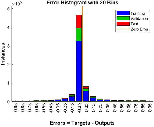
The total error of the output nodes was summed for training, validation, and testing, as shown in Figure 9. The histogram compares the frequency of the output classification error over 1,000 epochs and reports the number of instances. Error histogram was the histogram of the errors between target values and predicted values after training the neural network. As these error values indicated how predicted values differed from the target values, these were negative.

FIGURE 9

FIGURE 9. Error histogram with maximum classification accuracy.

The results showed that the working prototype of the electronic nose performed exceptionally well in the sample data collection. The trained neural network was successfully able to classify the samples to within 11.7% (error on average) of the actual beer samples. It successfully classified four beers with 88.3% accuracy. The neural network could compensate for a giant floating baseline and the limited amount of data with only 28 samples. The low number of models also restricted the true potential of the network to become fully developed. For this particular four-input, four-output system, the best performance was achieved with 5,000 hidden nodes based on features extracted from the whole curve with training–validation–test data of 70%-15%-15%.

4 Conclusion

A new portable modular design of an electronic nose was created to classify four different brands of Chinese beers based on their odor or aroma. The working prototype of this electronic nose featured an array of 4 MOS sensors that were commercially available from Figaro Engineering Inc. A fully automatic sample delivery system was designed with two air pumps and two solenoid air valves sourced from the local companies. A fully automated software-based data acquisition system was also developed, which required the electronic nose to connect to processing software through a PC. Data were then recorded in a CSV file.

Totally, 28 experiments were performed to collect the data for feature extraction. Over 70 tests were performed in MATLAB with different parameters in the neural network. Classification accuracy of the trained neural network drastically improved with the increase in hidden neurons with maximum precision of 88.3% reported with 5,000 hidden neurons. The type of feature extraction also affected the overall accuracy of classification. The amount of training, validation, and testing data also negatively affected the classification performance of the neural network. The best combination for maximum performance was determined as 70% training, 15% validation, and 15% testing data. Artificially doubling the data points also improved the classification performance, but it was not significant. The neural network exhibited only a 0.7% increase in its overall classification accuracy with double data points, and it took longer to train the network model. The neural network displayed a maximum classification performance of 88.3% with 5,000 hidden neurons and features extracted from the original response curve.

Data Availability Statement

The raw data supporting the conclusions of this article will be made available by the authors, without undue reservation.

Author Contributions

IZ designed the system, did the experiments, and wrote the manuscript. YC guided the algorithm in this paper. QB did partly the experiment. YY improved grammar and vocabulary. All authors reviewed the manuscript.

Conflict of Interest

The authors declare that the research was conducted in the absence of any commercial or financial relationships that could be construed as a potential conflict of interest.

Publisher’s Note

All claims expressed in this article are solely those of the authors and do not necessarily represent those of their affiliated organizations, or those of the publisher, the editors, and the reviewers. Any product that may be evaluated in this article, or claim that may be made by its manufacturer, is not guaranteed or endorsed by the publisher.

References

1. Falasconi M, Concina I, Gobbi E, Sberveglieri V, Pulvirenti A, Sberveglieri G. Electronic Nose for Microbiological Quality Control of Food Products. Int J Electrochem (2012) 2012:1–12. doi:10.1155/2012/715763

CrossRef Full Text | Google Scholar

2. Gliszczyńska-Świgło A, Chmielewski J. Electronic Nose as a Tool for Monitoring the Authenticity of Food. A Review. Food Anal. Methods (2017) 10(6):1800–16. doi:10.1007/s12161-016-0739-4

CrossRef Full Text | Google Scholar

3. Wojnowski W, Majchrzak T, Dymerski T, Gębicki J, Namieśnik J. Portable Electronic Nose Based on Electrochemical Sensors for Food Quality Assessment. Sensors (2017) 17(12):2715. doi:10.3390/s17122715

PubMed Abstract | CrossRef Full Text | Google Scholar

4. Eusebio L, Capelli L, Sironi S. Electronic Nose Testing Procedure for the Definition of Minimum Performance Requirements for Environmental Odor Monitoring. Sensors (2016) 161548(9):1548. doi:10.3390/s16091548

PubMed Abstract | CrossRef Full Text | Google Scholar

5. Liu Q, Li X, Ye M, Ge SS, Du X. Drift Compensation for Electronic Nose by Semi-supervised Domain Adaption. IEEE Sensors J. (2014) 14(3):657–65. doi:10.1109/JSEN.2013.2285919

CrossRef Full Text | Google Scholar

6. Vergara A, Vembu S, Ayhan T, Ryan MA, Homer ML, Huerta R. Chemical Gas Sensor Drift Compensation Using Classifier Ensembles. Sensors Actuators B Chem (2012) 166-167:320–9. doi:10.1016/j.snb.2012.01.074

CrossRef Full Text | Google Scholar

7. Lei Zhang L, Zhang D. Domain Adaptation Extreme Learning Machines for Drift Compensation in E-Nose Systems. IEEE Trans. Instrum. Meas. (2015) 64(7):1790–801. doi:10.1109/TIM.2014.2367775

CrossRef Full Text | Google Scholar

8. Zhang L, Tian F, Liu S, Dang L, Peng X, Yin X. Chaotic Time Series Prediction of E-Nose Sensor Drift in Embedded Phase Space. Sensors Actuators B Chem (2013) 182:71–9. doi:10.1016/j.snb.2013.03.003

CrossRef Full Text | Google Scholar

9. Dutta R, Kashwan KR, Bhuyan M, Hines EL, Gardner JW. Electronic Nose Based Tea Quality Standardization. Neural Netw(2003) 16(5):847–53. doi:10.1016/S0893-6080(03)00092-3

PubMed Abstract | CrossRef Full Text | Google Scholar

10. Lozano J, Santos JP, Horrillo MC. Wine Applications with Electronic Noses. In: ML Rodríguez Méndez, editor. Chapter 14 - Wine Applications with Electronic Noses. Electronic Noses and Tongues in Food Science. San Diego: Academic Press (2016). p. 137–48. doi:10.1016/B978-0-12-800243-8.00014-7

CrossRef Full Text | Google Scholar

11. Zhang L, Tian F, Zhang D. E-nose Algorithms and Challenges. In: Electronic Nose: Algorithmic Challenges. Singapore: Springer (2018). p. 11–20. doi:10.1007/978-981-13-2167-2_2

CrossRef Full Text | Google Scholar

12. Qi P-F, Zeng M, Li Z-H, Sun B, Meng Q-H. Design of a Portable Electronic Nose for Real-Fake Detection of Liquors. Rev. Sci. Instrum. (2017) 88(9):095001. doi:10.1063/1.5001314

PubMed Abstract | CrossRef Full Text | Google Scholar

13. Pádua A, Osório D, Rodrigues J, Santos G, Porteira A, Palma S, et al. Scalable and Easy-To-Use System Architecture for Electronic Noses. In: Proceedings of the 11th International Joint Conference on Biomedical Engineering Systems and Technologies. 1. BIODEVICES (2018). p. 179–86. doi:10.5220/0006597101790186

CrossRef Full Text | Google Scholar

14. Li C, Li H, Xie W, Du J. A S-type Bistable Locally Active Memristor Model and its Analog Implementation in an Oscillator Circuit. Nonlinear Dyn(2021) 106(1):1041–58. doi:10.1007/s11071-021-06814-4

CrossRef Full Text | Google Scholar

15. Ma XJ, Mou J, Liu J, Ma CG, Yang FF, Zhao X. A Novel Simple Chaotic Circuit Based on Memristor-Memcapacitor. Nonlinear Dyn100(3):2859. doi:10.1007/s11071-020-05601-x

CrossRef Full Text | Google Scholar

16. Li C-L, Zhou Y, Li H-M, Feng W, Du J-R. Image Encryption Scheme with Bit-Level Scrambling and Multiplication Diffusion. Multimed Tools Appl (2021) 80:18479–501. doi:10.1007/s11042-021-10631-7

CrossRef Full Text | Google Scholar

17. Li XJ, Jun Mou J, Banerjee S, Cao YH. An Optical Image Encryption Algorithm Based on Fractional-Order Laser Hyperchaotic System. Int J Bifurcation Chaos (2022) 32(03):2250035. doi:10.1142/s0218127422500353

CrossRef Full Text | Google Scholar

18. Gao X, Mou J, Xiong L, Sha Y, Yan H, Cao Y. A Fast and Efficient Multiple Images Encryption Based on Single-Channel Encryption and Chaotic System. Nonlinear Dyn(2022) 108:613–36. doi:10.1007/s11071-021-07192-7

CrossRef Full Text | Google Scholar

19. Gao X, Mou J, Banerjee S, Cao Y, Xiong L, Chen X. An Effective Multiple-Image Encryption Algorithm Based on 3D Cube and Hyperchaotic Map. J King Saud Univ - Comput Inf Sci (2022) 34(Issue 4):1535–51. doi:10.1016/j.jksuci.2022.01.017

CrossRef Full Text | Google Scholar

20. Li C, Yang Y, Yang X, Zi X, Xiao F. A Tristable Locally Active Memristor and its Application in Hopfield Neural Network. Nonlinear Dyn(2022) 108:1697–717. doi:10.1007/s11071-022-07268-y

CrossRef Full Text | Google Scholar

21. Lin H, Wang C, Hong Q, Sun Y. A Multi-Stable Memristor and its Application in a Neural Network. IEEE Trans. Circuits Syst. II (2020) 67(12):3472–6. doi:10.1109/TCSII.2020.3000492

CrossRef Full Text | Google Scholar

22. Kim M-H, Park H-L, Kim M-H, Jang J, Bae J-H, Kang IM, et al. Fluoropolymer-based Organic Memristor with Multifunctionality for Flexible Neural Network System. npj Flex Electron (2021) 5:34. doi:10.1038/s41528-021-00132-w

CrossRef Full Text | Google Scholar

23. Luo YX, She K, Yu K, Yang L. Research on Vehicle Logo Recognition Technology Based on Memristive Neural Network. J Inf Secur Res (2021) 7(No 8):715

Google Scholar

24. Little RL. Neural Network Compound Predictor for Spirits in an Electronic Nose. Ontario, Canada: The University of Guelph (2014). p. 22

Google Scholar