Assessment of the Variational Quantum Eigensolver: Application to the Heisenberg Model

We present and analyze large-scale simulation results of a hybrid quantum-classical variational method to calculate the ground state energy of the anti-ferromagnetic Heisenberg model. Using a massively parallel universal quantum computer simulator, we observe that a low-depth-circuit ansatz advantageously exploits the efficiently preparable Néel initial state, avoids potential barren plateaus, and works for both one- and two-dimensional lattices. The analysis reflects the decisive ingredients required for a simulation by comparing different ansätze, initial parameters, and gradient-based versus gradient-free optimizers. Extrapolation to the thermodynamic limit accurately yields the analytical value for the ground state energy, given by the Bethe ansatz. We predict that a fully functional quantum computer with 100 qubits can calculate the ground state energy with a relatively small error.

1 Introduction

Variational methods, in particular the variational quantum eigensolver (VQE) [1, 2], have recently been successful in demonstrating to solve proof-of-concept problems on current quantum computing devices [3–5]. Despite the initial success, it remains an open question which problems would demonstrate an advantage on future quantum computers. Finding the ground state energy of the Heisenberg model is one of the candidates.

Recent works have focused on the implementation of the VQE on quantum computers, including the invention of efficient methods for current devices [5, 6], the reduction of the total number of required qubits [7, 8], the testing of optimization algorithms [9, 10], and a study of the effects of noise [11]. Also, attempts to implement the Bethe ansatz [12] on a quantum computer [13, 14] have been made. Results for implementations of the VQE on quantum computers with up to 20 qubits [15] or less [16–19] are available.

Despite the progress in hybrid quantum-classical variational methods, several of their important aspects are still unexplored. Large-scale simulations of VQE for calculating the ground state energy of the Heisenberg model have not yet been performed. It is unclear if a single ansatz can be used for both the one- and two-dimensional lattices. A clear picture of how the minimum energy scales by using a certain ansatz within and beyond what is emulatable on classical hardware is missing. In this work, we present results for all these aspects.

The rest of the paper is structured as follows. In Section 2, we briefly review the variational principle and the Heisenberg model, and introduce the ansatz. In Section 3, we present the results of our work for one- and two-dimensional lattices. Finally, in Section 4, we summarise our findings.

2 Theory

2.1 Variational Principle

The variational principle states that the energy E obtained by using a certain parameterized wavefunction ψ(θ) for a problem Hamiltonian H is a strict upper bound to the ground state energy E₀ of H:

$E=⟨\psi \left(\theta \right)|H|\psi \left(\theta \right)⟩\ge E_0.(1)$

The VQE uses the variational principle, Eq. 1, to compute E₀ of H on a quantum computer. The VQE algorithm is a hybrid quantum-classical algorithm that utilizes resources from quantum and classical computers in an iterative process. The diagram depicted in Figure 1 shows the link between the quantum processing unit (QPU) and the classical processing unit (CPU). The QPU is responsible for carrying out the computation for a certain quantum circuit that generates the state ψ(θ), depending on a set of parameters, and returns the corresponding bitstrings to the CPU obtained after the measurement. The bitstrings are accumulated and processed by the classical unit, fed to an optimizer that suggests the next set of parameters that will lower the energy in successive iterations.

FIGURE 1

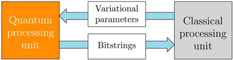
FIGURE 1. (Colour online) Schematic of the hybrid quantum-classical mechanism of a variational quantum eigensolver.

2.2 Heisenberg Model

We analyze the Hamiltonian representing the quantum spin model

$H=\sum _{i>j}^N\left(J_{ij}^{xx}{\sigma }_i^x\cdot {\sigma }_j^x+J_{ij}^{yy}{\sigma }_i^y\cdot {\sigma }_j^y+J_{ij}^{zz}{\sigma }_i^z\cdot {\sigma }_j^z\right),(2)$

where N denotes the number of spins, and σ^x, σ^y, and σ^z are the Pauli matrices. Throughout the rest of the paper, we use units such that ℏ = 1 and J’s are dimensionless. If $J_{ij}^{\alpha \alpha }=1$ for all i, j = 1, … , N, and α ∈ {x, y, z}, we call H the isotropic anti-ferromagnetic Heisenberg model Hamiltonian. If all coefficients $J_{ij}^{\alpha \alpha }$ are chosen randomly in the interval ($\left(\right.\mathrm{0,1}\left.\right]$], then we call H the random Hamiltonian. We use both open and periodic boundary conditions and map each spin to a qubit. For most of our simulations we consider bipartite spin lattices with a single exception of a (frustrated) triangular spin lattice.

2.3 Ansatz

In general, the final state of a system acted upon by a parametrized ansatz can be written in the form

$|{\psi }_f\left(\mathit{\theta }\right)\rangle =U\left(\mathit{\theta }\right)|{\psi }_0\rangle ,(3)$

where θ are the variational parameters, U is the ansatz, and |ψ₀⟩ denotes the initial state. In this paper we demonstrate that the following ansatz is sufficient to yield an accurate approximation to the ground state energy.

$U\left(\mathit{\theta }\right)=\left[\prod _{l=N-1}^1\prod _{k=N}^{l+1}{U}_{lk}\left({\theta }_{lk}\right)\right]\left[\prod _{l=N-1}^1\prod _{k=N}^{l+1}{U}_{kl}\left({\theta }_{kl}\right)\right],(4)$

where

$U_{pq}\left({\theta }_{pq}\right)=\left\{\begin{array}{cc}{e}^{-i{\theta }_{pq}{\sigma }_p^y{\sigma }_q^x}\hfill & \text{if}p=N\text{or}q=N,\hfill \\ e^{-i{\theta }_{pq}{\sigma }_p^y{\sigma }_q^x{\sigma }_N^z}\hfill & \text{otherwise.}\hfill \end{array}\right.(5)$

We elaborate on how to expand Eq. 4. There is an independent index l and a dependent index k. The index l is monotonically decreased from N − 1 to 1. For each value of l, the dependent index k is decreased from N to l + 1. The index l is not decremented until all the values of k are enumerated. These values of l and k describe the indices of the qubits that the operators in Eq. 5 act upon. In every operator, no more than three qubits are involved. The corresponding parameters θ_kl are independent for each unique combination of l and k. The parameters θ_kl affect the phase of the Nth qubit. The number of unitary operators in Eq. 4 is given by N(N − 1). The ordering of the unitary operators is important. In this paper, the specific combination of the operators in Eq. 5 is termed the XY-ansatz. Any other ordering is prone to produce results which may be different from each other. This is consistent with the findings in recent literature [20, 21].

The motivation to keep the number of operators to a maximum of two or three is inspired from the coupled cluster ansatz which can be powerful enough to express relevant states even in this restrictive form [2]. It is then intuitive to try this approach also for the Heisenberg model. Accordingly, such an ansatz is expressed by

$|{\psi }_f\left(\mathit{\theta }\right)\rangle =e^{-iA\left(\mathit{\theta }\right)}|{\psi }_0\rangle ,(6)$

where A can contain sums of products of Pauli operators. The implementation of an ansatz, e.g. the one given by Eq. 6, is not a simple task in general as it requires factorization of the matrix exponential e^−iA(θ) [22]. Factorization creates a series of products of unitary operations, which results in deeper quantum circuits with a large number of gates. In this work, we do not directly implement the ansatz given by Eq. 6, but seek for other ansätze in a factorized form which do not require further factorization. In effect, we create a quantum circuit from a set of operators instead of a sum of operators. Such an approach allows us to build low-depth quantum circuits. Furthermore, from an experimental perspective, it is difficult to build a quantum computing device in which all the qubits work equally well. Some qubits may perform certain gates more efficiently than others. In order to exploit such devices efficiently and to accommodate for experimental imperfections, we proposed the ansatz where all the parameterized gates are placed on only one qubit. All operations of the parametrised gates can be restricted to this single qubit.

For comparison with the XY-ansatz, we consider two different ansätze. The first one is inspired by quantum chemistry. The unitary coupled cluster ansatz restricted to single and double excitations (UCCSD) is shown to produce results with chemical accuracy [23–26]. We consider

$U\left(\mathit{\theta }\right)=\prod _{l=N-1}^1\prod _{k=N}^{l+1}{U}_{kl}\left({\theta }_{kl}\right),(7)$

where

$U_{kl}\left({\theta }_{kl}\right)=\left\{\begin{array}{cc}\prod _{\alpha }\prod _{\beta }{e}^{-i{\theta }_{kl}^{\beta \alpha }{\sigma }_k^{\beta }{\sigma }_l^{\alpha }}\hfill & \text{if}k=N\text{or}l=N,\hfill \\ \prod _{\alpha }\prod _{\beta }{e}^{-i{\theta }_{kl}^{\beta \alpha }{\sigma }_k^{\beta }{\sigma }_l^{\alpha }{\sigma }_N^z}\hfill & \text{otherwise,}\hfill \end{array}\right.(8)$

where α, β ∈ {x, y, z}. A combinatorial calculation shows that the number of unitary operators in Eq. 7 is given by 3²N!/2!(N − 2)!. Although the total number of terms scales polynomially rather than exponentially, further reductions are always welcome since the redundant terms often slow down the optimization process. Clearly, the operators in Eq. 4 are a subset of those in Eq. 7. The differences between using these two are highlighted in the results section.

The second ansatz is inspired by the problem Hamiltonian. We consider the ansatz which for the one-dimensional lattice Hamiltonians is given by

$U\left(\mathit{\theta }\right)=U_p\left({\mathit{\theta }}_p\right)\dots U_1\left({\mathit{\theta }}_1\right),(9)$

where U_p is given

$U_p\left({\mathit{\theta }}_p\right)=\prod _{k=1}^N{U}_{kp}\left({\mathit{\theta }}_{kp}\right),(10)$

and periodic boundary conditions are used. Each U_kp(θ_kp) is given by

$U_{kp}\left({\mathit{\theta }}_{kp}\right)=\left\{\begin{array}{cc}\prod _{\alpha }{e}^{-i{\theta }_k^{\alpha }{\sigma }_k^{\alpha }{\sigma }_{k+1}^{\alpha }}\hfill & \text{if}k=N\text{or}k+1=N,\hfill \\ \prod _{\alpha }{e}^{-i{\theta }_k^{\alpha }{\sigma }_k^{\alpha }{\sigma }_{k+1}^{\alpha }{\sigma }_N^z}\hfill & \text{otherwise.}\hfill \end{array}\right.(11)$

For a lattice of size N in one-dimension, the ansatz in Eq. 9 has p × 3N unitary operators. The variational Hamiltonian ansatz [27] is itself inspired from adiabatic evolution. The idea is that a combination of ansatz and initial parameters that mimics the adiabatic evolution can have a lower initial energy to start the variational optimization. It has been used for solving the Hubbard-Fermi model [28, 29] and a modified Haldane-Shastry Hamiltonian [30].

A good choice for the initial state |ψ₀⟩ often yields better variational results. In the case of antiferromagnets, a good |ψ₀⟩ for the bipartite lattices is known to be the Néel state where one sublattice is initialised with spins anti-parallel to the other sublattice. The Néel state, for an even number of spins, is in the magnetic sector of zero magnetization, where the ground state for the one-dimensional isotropic anti-ferromagnetic Heisenberg model is located. For the frustrated lattice, half of the lattice spins are initialised anti-parallel to the other half, without regard to their location in the lattice. The qubits representing the spins for one group are initialised as zeros and those in the other group (anti-parallel) as ones.

2.4 Implementation

We use the massively parallel simulator Jülich Universal Quantum Computer Simulator (JUQCS) [31, 32] to perform operations on the state vector. We also use Qiskit [33] for small problem sizes. In an actual quantum device, the state vector itself is not accessible. Instead, the quantum device will produce an ensemble of bitstrings consisting of 0 and 1s only, from which the expectation values of the observables can be derived. This raises two issues. First, since the number of samples or bitstrings can only be finite, it is not always clear if finite sampling can accurately represent the underlying probability distribution. Second, we need a procedure to measure the individual terms of the Hamiltonian. While the first is an open problem, recent works have developed efficient methods for the second when it becomes a problem [34–38]. Fortunately, both these problems do not hinder finding the ground state energy of the Heisenberg model. First, on an actual quantum device, we do not need explicit knowledge of the probability distribution; one can calculate the expectation values directly by sampling. From the samples we can estimate the energy with an accuracy proportional to the square root of the number of samples. Second, unlike in quantum chemistry, the measurement of individual terms for the Heisenberg model is not a problem.

The implementation of the ansatz is best understood through an example. Consider the four-qubit circuit shown in Figure 2, implementing the XY-ansatz for the N = 4 isotropic Heisenberg ring (see Eq. 2). There are 12 parameters in total, and Figure 2 shows the implementation of the first three. After the initial state preparation, gates are applied to construct the unitary operators. The circuit in the rectangular solid box corresponds to the implementation of the $\exp (-i{\theta }_{43}^{yx}{\sigma }^z\cdot {\sigma }^z)$ operator having a variational parameter ${\theta }_{43}^{yx}$. The terms containing σ^x and σ^y are implemented by changing to the appropriate basis. The rectangular dashed box highlights the implementation of the third term in the ansatz, given by $\exp (-i{\theta }_{32}^{yx}{\sigma }_3^y\cdot {\sigma }_2^x\cdot {\sigma }_4^z)$. Although the results for the special case of four qubits can be achieved using an even smaller subset of terms in the XY-ansatz operators containing only five parameters, for consistency and completeness, the twelve parameters are used for all the cases. The simulation for this example using Qiskit and JUQCS gives the energy −8.0, which is also the theoretical value obtained by exact diagonalization. The final state also has a 100% overlap with the ground state. The corresponding z- and total-magnetization were both zero, as required.

FIGURE 2

FIGURE 2. Circuit showing the first three parameters for a four-qubit XY-ansatz. The $R_x^{+},R_x^{-}$, and $R_y^{+},R_y^{-}$ gates are R_x(π/2), R_x( −π/2), and R_y(π/2), R_y( −π/2), respectively. The parameterized gate is always placed on the last qubit. Gates in the solid box correspond to the $e^{-i\theta {\sigma }^z\cdot {\sigma }^z}$ operator. Gates in the dashed box implement $e^{-i\theta {\sigma }^y\cdot {\sigma }^x\cdot {\sigma }^z}$. The shown circuit is unoptimized and is optimized before usage.

For the classical optimisation part of the VQE, we use the sequential least squares quadratic programming (SLSQP) [39] optimizer in the SciPy package [40]. SLSQP is a quasi-Newton gradient based algorithm. When using an ideal simulator, the gradients are computed numerically using the cost-effective forward differences formula. The calculation of the energy for given values of the parameters involves the quantum subroutine of VQE. Once the energies are obtained, the calculation of the gradient is done on the classical computer. Calculation of gradient and the next iterate is not a hard problem and classical computers can be used. It is the calculation of the energy for which quantum resources will be required. In our work, the cost of gradient computation for the optimizer is included in the total energy evaluations. For comparison, we also use a gradient-free optimizer called constrained optimization by linear approximation (COBYLA) [40–42].

3 Results

3.1 One-Dimensional Lattices

The results for the one-dimensional isotropic Hamiltonians with periodic boundary conditions are shown in Figure 3A. The coloured lines show the optimization progress, i.e. the lowest energy achieved by successive energy evaluations for different lattice sizes. Initially, the system is in the Néel state. To take advantage of the Néel state, all the optimization parameters are initialised as zeros. As the optimization proceeds, the drop in energy is visible for all lattice sizes shown. The stepped progression is characteristic of the quasi-Newton optimization algorithms, which calculate the gradient before deciding on the step size. Each “step” of the staircase corresponds to a length equal to the number of parameters, since the formula of the forward differences for calculating the gradients requires N (N − 1) + 1 energy evaluations, where N (N − 1) is the number of parameters. Below each optimization curve is a horizontal black line corresponding to the energy of the ground state, obtained numerically by the Lanczos algorithm. According to the variational principle, the calculated energies are upper bounds to the energy of the ground states. Starting from a lattice with 14 spins, the optimizer gave no signal for termination, but due to a time limit of 24 h on the supercomputer [43], the calculations stopped. Due to the different number of compute nodes, circuit depths, and parameters, the total number of energy evaluations differs for each lattice size. The energy optimization process can be restarted from the last values of the parameters. An example is shown for the lattice with 25 spins, as can be seen from the longer curve resulting from the extra energy evaluations. In all the cases shown, the XY-ansatz produced a final energy E_f, which is close to the ground state energy.

FIGURE 3

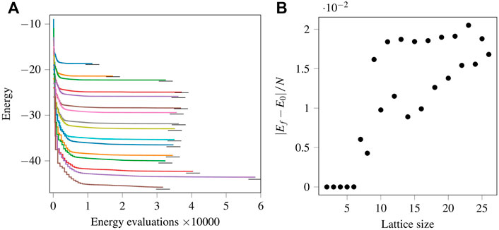
FIGURE 3. (Colour online) (A): Optimization progress using the XY ansatz for 11 spins (first line), 12 spins (second line) and so on, up to 26 spins (bottom line). The small horizontal black lines represent the ground state energy. (B): Absolute difference in the variational and ground state energy per spin for different spins or lattice size.

The absolute difference between E_f and the corresponding ground state energy E₀ per spin for each lattice size is shown in Figure 3B. Results up to the lattice size of 6 spins match exactly with the ground state energy [data not shown in (A)], and the differences show up for N ≥ 7. The points cluster in two groups, one corresponding to lattices with an even and another one with an odd number of spins. We observe that the final energies for the lattices with an even number of spins are lower than for the ones with an odd number of spins. Additionally, we note that the ground states of the systems with an odd number of spins are degenerate. Through the variational principle, the ground state energies are mapped to the global minima of an energy landscape when an ansatz can express the ground state. There may be multiple global minima for degenerate cases. Due to this reason the energy landscape will be different from the even spin cases. Therefore, we conjecture that finding the ground state of degenerate cases using VQE is more challenging. This is also observed in the simulations we performed.

Figure 4A shows the energy optimization progress using two different sets of initial parameters. The legend indicates the lattice size. The lines can be separated into two groups, top (dashed) and bottom (solid). The bottom group corresponds to the case where the parameters were initialised as zeros, thus taking advantage of the Néel state and starting from a lower energy value. The top group of lines corresponds to parameters initialised as randomly distributed values in the interval ($\left[\right.\mathrm{0,2}\pi \left.\right)$], not taking advantage of the Néel state and starting from a much higher energy, often close to E = 0. For all lattice sizes, initializing the parameters as zeros yields large drops in energy for the first few iterations, and E_f is close to the ground state energy. After the significant drop, the (relative) progress slows down as the energy landscape becomes flatter near a minimum, and a large number of iterations is required to decrease the energy further. On the other hand, random initializations of the parameters do not yield significantly big drops in the energy in any of the cases. A prohibitively large number of energy evaluations seems required to obtain the same accuracy as when parameters are initialised as zeros. From a practical perspective, starting from random parameters does not appear to be very useful for the current problem.

FIGURE 4

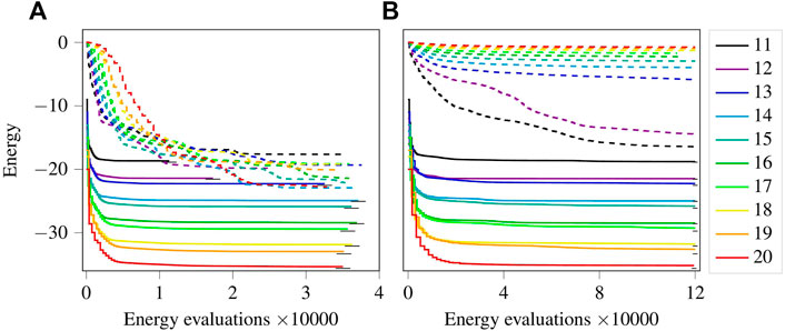
FIGURE 4. (Colour online) (A): Progress comparison when initializing with zeros (solid lines) versus random values (dashed lines) as parameters for the XY-ansatz. (B): Same as (A), except for using the ansatz given by Eq. 7. Legend depicts the lattice size for both (A,B). The small horizontal black lines represent the ground state energy.

Figure 4B shows the energy optimization progress using the UCCSD inspired ansatz given by Eq. 7. Similar to plot (A), plot (B) shows the trend corresponding to the two different initializations of the parameters. Initializing all parameters as zeros is observed to have a significant initial drop in the energy, contrary to the random parameters. Interestingly, energy optimization progresses for cases with random initial parameters appear to be slower in proportion to the increasing lattice size, i.e. larger N have a slower drop in energy. This effect appears to be consistent with what is termed in the recent literature as the barren-plateau [44–47]. The larger lattice sizes, which require a larger number of parameters, lead to vanishingly small gradients. Given that vanishingly small gradients appear when one approaches a minimum, it is difficult to determine whether the random parameters landed in a local minimum of the energy landscape or at a barren-plateau. One way to find this out would be to restart multiple times with new sets of random parameters, but given that the barren-plateau effect is something that one aims to avoid, which is possible by initializing all parameters as zeros in this case, we skip such an approach.

In both plots (A) and (B) in Figure 4, for parameters initialised as zeros, E_f is very close to the ground state energy. This is understandable as the terms in the XY-ansatz are a subset of the terms given in Eq. 7. However, the difference between the two lies in the number of energy evaluations required to reach the ground state energy. The energies obtained with the XY-ansatz have the same (or comparable) values as the energies obtained with the UCCSD inspired ansatz, but much less energy evaluations with fewer parameters.

Despite the success of initializing the parameters as zeros, it should be noted that such an approach does not necessarily give the lowest possible energy given the ansatz. We performed random initializations with one hundred sets of random parameters for the smaller lattices. The results are shown in Figure 5A. We count and plot the number of cases in which the energy found by starting the optimiser using random initial parameters obtained a final energy equal to or lower than that obtained when starting from the Néel state. We observe that the cases drop sharpy as the lattice size increases. However, finding even a single energy lower than that found when starting from the Néel state shows that the minimum energy reached by initializing all parameters as zeros, although being very close to the ground state energy, is still only a local minimum and usually not a global minimum.

FIGURE 5

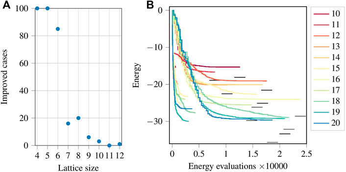
FIGURE 5. (Colour online) (A): The number of cases where the final energy obtained using random initial parameters was either equal to or lower than the energy obtained by setting zeros as initial parameters. (B): Optimization progress for the ansatz given by Eq. 9 for p = 1 (group of shorter lines on the left) and p = 5 (group of longer lines on the right). The legend shows the lattice size. The short horizontal black lines represent the ground state energy.

Figure 5B shows the energy optimization progress using the ansatz given by Eq. 9. The lines can again be divided into two groups. The shorter lines on the left correspond to p = 1 and the long lines on the right to p = 5. The lines for p = 5 are longer simply because in this case there are five times more parameters than for p = 1, and so five times more energy evaluations are required to compute the gradient per iteration. For this ansatz, the parameters need to be initialised randomly since initializing them with zeros (for the tested cases with N ≤ 10) results in the optimizer being trapped in a local minimum at the first iteration. It is observed that simply increasing the number of parameters in the circuit is no guarantee for improving the minimum energy. While for the lattice with 19 spins a lower energy is reached with p = 1 than with p = 5, the opposite is the case for the lattice with 20 spins. While a larger parameter space may facilitate a broader spectrum of states, the energy landscape may be the cause of this observation as local minima may surround the global minimum and impede reaching it. Since a random initialization would not be able to take advantage offered by the Néel state, and would thus require a much larger number of energy evaluations to converge to E_f, we restrict our study to only one such random initialization.

Figure 6A shows the energy optimization progress for the random case of the anti-ferromagnetic one-dimensional ring. Using the XY-ansatz, the parameters were initialised as zeros. Except for the ring with 10 spins, none of the optimization processes signalled convergence, and the optimization could be continued to reduce the energy further if required. A quick drop in the initial energy is also observed for the random case, and all the energies are reasonably close to the ground state energy.

FIGURE 6

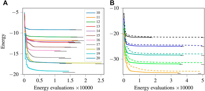
FIGURE 6. (Colour online) (A): Energy optimization progress using the XY-ansatz for different Hamiltonians with random coupling interactions for the different numbers of spins shown in legend. (B): Energy optimization progress using gradient-based (solid lines) and gradient-free (dashed lines) optimizers for rings with isotropic couplings between the spins with 12 spins (first pair of the lines from top), 14 spins (second pair of lines from the top), and so on up to 20 spins (last pair of lines at the bottom). The short horizontal black lines represent the ground state energy.

Figure 6B shows the energy optimization progress using the gradient-based optimizer SLSQP (solid lines) and the gradient-free optimizer COBYLA (dashed lines). We only show the results for the even lattice sizes. The results for the odd lattice sizes are similar. The gradient-based method gives lower energies at each energy evaluation and finds a much lower minimum faster than the gradient-free method. This result confirms the commonly accepted notion that for noiseless functions, gradient-based methods are superior.

3.2 Two-Dimensional Lattices

We apply the XY-ansatz without any changes. Results for an isotropic ladder Hamiltonian with open boundary conditions are shown in Figure 7A. The results show the energy optimization progress for ladders of size 3 × 2 up to size 13 × 2. For example, the 8 × 2 ladder, where the optimizer did not converge even after two runs of continued optimization, reported E_f/N = −2.212 as compared to the ground state energy per spin E₀/N = −2.229.

FIGURE 7

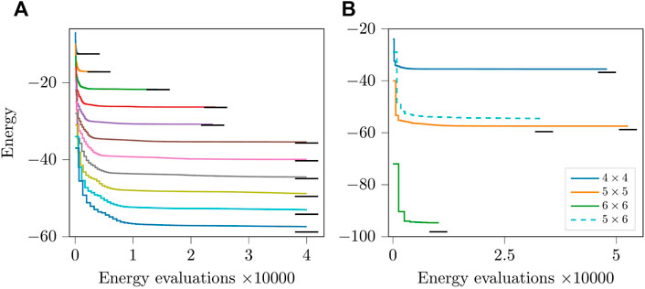
FIGURE 7. (Colour online) (A): Energy optimization progress for isotropic ladders with open boundary conditions. The top line is for a lattice with 3 × 2 spins, the second for one with 4 × 2 spins and so on until the bottom line which is for a lattice with 13 × 2 spins. (B) Energy optimization progress for two-dimensional square lattices of size 4 × 4 and 5 × 5 with open boundary conditions and 6 × 6 with periodic boundary conditions. The dashed line is for a frustrated triangular lattice of dimensions 5 × 6 with open boundary conditions. The short horizontal black lines represent the ground state energy.

Figure 7B shows results for three cases with square lattices and a 5 × 6 (frustrated) triangular lattice. The 4 × 4 and 5 × 5 lattices had open boundary conditions and the final energies were E_f/N = −2.218 and E_f/N = −2.298 as compared to E₀/N = −2.297 and E₀/N = −2.351, respectively. The optimized (unoptimized) circuit depths were 805 (1398) and 1939 (3531), respectively. For the frustrated lattice, E_f/N = −1.817 as compared to E₀/N = −1.986. The results for the frustrated lattice show a slightly larger gap in the energy obtained and the ground state. This could either be explained by assuming that the ansatz is less suitable for the case with the frustrated lattice or that the energy obtained when initializing all parameters as zeros corresponds to a local minimum far away from the global minimum.

The case of the square lattice of size 6 × 6 with periodic boundary conditions poses a specific difficulty with the parameter optimization. The problem is that the XY-ansatz for 36 spins has 1260 parameters, and only one iteration can be performed as the evaluation of the gradient is possible only once within 24 h, the time per job on the supercomputer. Since the quasi-Newton methods require multiple iterations without losing the internal variables that systematically improve the convergence per iteration, the optimization is ill-suited for larger problems that cannot undergo multiple iterations in one run. However, this problem can be avoided by saving the internal variables of the optimizer, but this approach is beyond the scope of this work. Despite such a drawback, we proceeded with the first few iterations without saving the internal variables and were able to see a reasonable drop in the initial energy. The circuit depth after optimizing the circuit was reduced from 7458 to 3985. The final energy was E_f/N = −2.631 as compared to E₀/N = −2.715.

3.3 Extrapolation

The energies obtained for the one-dimensional lattices can be fitted to a line for extrapolation, as shown in Figure 8A. The slope of the line that gives the energy per spin in the thermodynamic limit, is −1.7783, which can be compared to the exact value −1.7726, known from the Bethe ansatz [48]. The reported value only differs from the exact value by 5.7 × 10⁻³. Note that while the variational theorem guarantees that the energy obtained is a strict upper bound to the ground state, this is not necessarily the case when estimating the value in the thermodynamic limit by means of a fitted extrapolation.

FIGURE 8

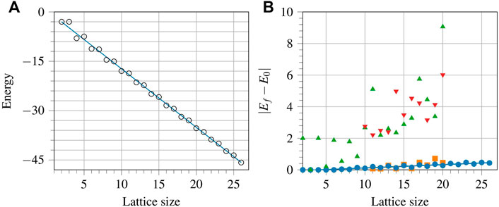
FIGURE 8. (Colour online) (A): Least squares fitting to the variational energies obtained for the one-dimensional isotropic rings of different sizes. The slope of the line, − 1.7783, gives the energy for the infinite ring case. (B): Absolute differences of the variational and ground state energies for different lattice sizes for the isotropic rings using the ansatz from Eq. 9 with p = 1 (green triangles), p = 5 (red inverted triangles), the ansatz from Eq. 7 (orange squares), and the XY-ansatz (blue dots).

One measure of an ansatz’s ability to scale up beyond what classical computers can simulate is to predict, given the available data, the expected difference between the VQE and exact energies. Such a calculation can be performed by extrapolating the available data. Figure 8B shows data for four different ansätze, namely the ansatz from Eq. 9 with p = 1 (green triangles), p = 5 (red inverted triangles), the ansatz from Eq. 7 (orange squares), and the XY-ansatz (blue dots). Although some of the orange squares are lower than the corresponding blue dots, indicating that a lower energy was obtained using the ansatz from Eq. 7 compared to using the XY-ansatz, the difference is small, and the XY-ansatz is the preferred choice because its number of parameters is significantly smaller. For both the p values tested, the obtained data for the ansatz from Eq. 9 puts it out of competition with the XY-ansatz. Moreover, there is no clear pattern that may help predict the behaviour for the ansatz from Eq. 9 beyond the available data. Linear fitting is performed for the XY-ansatz, and the slope is equal to 2.0829 × 10⁻² with the intercept −8.6202 × 10⁻². Using the given slope, we predict that for a 100-spin ring, the expected energy per spin will be higher than the ground state energy per spin by a value of approximately 0.02.

4 Conclusion

We calculated the minimum energy for various implementations of the Heisenberg model for the one- and two-dimensional, isotropic, frustrated, and randomly-coupled lattices, using gradient-based and gradient-free optimizers, and different ansätze. The herein proposed XY-ansatz shows reasonable results if all the simulation variables are optimized, i.e. a suitable initial state combined with a good quality optimizer and a good choice of initial parameters.

Given an ansatz, there is currently no analytical method to ascertain if its global minimum corresponds to the ground state energy. Thus, we rely on optimization algorithms to navigate through the multi-dimensional rugged energy landscapes. In many such landscapes, there appear multiple local minima close to the ground state energy. For the cases where the exact ground state energy was not obtained using the XY-ansatz, it remains an open question if the global minimum of the energy landscape corresponds to the ground state energy. Thus, an improvement of the optimization algorithms appears to be essential for the further success of hybrid variational methods.

For the variational simulations performed in this work, initializing the variables as zeros instead of random numbers produced better results. For the anti-ferromagnetic Heisenberg model, it is known that the Néel state is an efficient initial state, and starting from zeros takes advantage of this knowledge. Therefore, in general, it is the knowledge or insight about a particular problem Hamiltonian that is relevant for an improved performance of the variational methods.

Data Availability Statement

The raw data supporting the conclusion of this article will be made available by the authors, without undue reservation.

Author Contributions

All authors contributed to the conception and design of the study. MJ implemented and performed the simulations and collected the data. FJ calculated the ground state energies using the Lanczos method. MJ wrote the first draft of the manuscript. All authors contributed to manuscript revision, read, and approved the submitted version.

Funding

MJ acknowledges support from the project OpenSuperQ (820363) of the EU Quantum Flagship.

Conflict of Interest

The authors declare that the research was conducted in the absence of any commercial or financial relationships that could be construed as a potential conflict of interest.

Publisher’s Note

All claims expressed in this article are solely those of the authors and do not necessarily represent those of their affiliated organizations, or those of the publisher, the editors and the reviewers. Any product that may be evaluated in this article, or claim that may be made by its manufacturer, is not guaranteed or endorsed by the publisher.

Acknowledgments

The authors gratefully acknowledge the Gauss Centre for Supercomputing e.V. (www.gauss-centre.eu) for funding this project by providing computing time [43].

References

1. Peruzzo A, McClean J, Shadbolt P, Yung MH, Zhou XQ, Love PJ, et al. A Variational Eigenvalue Solver on a Photonic Quantum Processor. Nat Commun (2014) 5:1. doi:10.1038/ncomms5213

PubMed Abstract | CrossRef Full Text | Google Scholar

2. McClean JR, Romero J, Babbush R, Aspuru-Guzik A. The Theory of Variational Hybrid Quantum-Classical Algorithms. New J Phys (2016) 18:023023. doi:10.1088/1367-2630/18/2/023023

CrossRef Full Text | Google Scholar

3. O’Malley PJJ, Babbush R, Kivlichan ID, Romero J, McClean JR, Barends R, et al. Scalable Quantum Simulation of Molecular Energies. Phys Rev X (2016) 6:031007. doi:10.1103/PhysRevX.6.031007

CrossRef Full Text | Google Scholar

4. Kokail C, Maier C, van Bijnen R, Brydges T, Joshi MK, Jurcevic P, et al. Self-Verifying Variational Quantum Simulation of Lattice Models. Nature (2019) 569:355–60. doi:10.1038/s41586-019-1177-4

PubMed Abstract | CrossRef Full Text | Google Scholar

5. Kandala A, Mezzacapo A, Temme K, Takita M, Brink M, Chow JM, et al. Hardware-Efficient Variational Quantum Eigensolver for Small Molecules and Quantum Magnets. Nature (2017) 549:242–6. doi:10.1038/nature23879

PubMed Abstract | CrossRef Full Text | Google Scholar

6. Huggins W, Patil P, Mitchell B, Birgitta Whaley K, Miles Stoudenmire E. Towards Quantum Machine Learning with Tensor Networks. Quan Sci Technology (2019) 4:024001. doi:10.1088/2058-9565/aaea94

CrossRef Full Text | Google Scholar

7. Liu J-G, Zhang Y-H, Wan Y, Wang L. Variational Quantum Eigensolver with Fewer Qubits. Phys Rev Res (2019) 1:023025. doi:10.1103/physrevresearch.1.023025

CrossRef Full Text | Google Scholar

8. Fujii K, Mitarai K, Mizukami W, Nakagawa YO. Deep Variational Quantum Eigensolver: a divide-and-conquer Method for Solving a Larger Problem with Smaller Size Quantum Computers. arXiv (2020) 2007:10917. doi:10.48550/arXiv.2007.10917

CrossRef Full Text | Google Scholar

9. Koczor B, Benjamin SC. Quantum Analytic Descent. arXiv (2021) 2008:13774. doi:10.48550/arXiv.2008.13774

CrossRef Full Text | Google Scholar

10. Ostaszewski M, Grant E, Benedetti M. Structure Optimization for Parameterized Quantum Circuits. Quantum (2021) 5:391. doi:10.22331/q-2021-01-28-391

CrossRef Full Text | Google Scholar

11. Zeng J, Wu Z, Cao C, Zhang C, Hou S-Y, Xu P, et al. Simulating Noisy Variational Quantum Eigensolver with Local Noise Models. Quan Eng (2021) 3:e77. doi:10.1002/que2.77

CrossRef Full Text | Google Scholar

12. Bethe H. Zur Theorie der Metalle. Z Physik (1931) 71:205–26. doi:10.1007/bf01341708

CrossRef Full Text | Google Scholar

13. Nepomechie RI. Bethe Ansatz on a Quantum Computer? arXiv (2020) 2010:01609. doi:10.48550/arXiv.2010.01609

CrossRef Full Text | Google Scholar

14. Van Dyke JS, Barron GS, Mayhall NJ, Barnes E, Economou SE. Preparing Bethe Ansatz Eigenstates on a Quantum Computer. PRX Quant. (2021) 2 (1:040329. doi:10.1103/PRXQuantum.2.040329

CrossRef Full Text | Google Scholar

15. Lyu C, Montenegro V, Bayat A. Accelerated Variational Algorithms for Digital Quantum Simulation of many-body Ground States. Quantum (2020) 4:324. doi:10.22331/q-2020-09-16-324

CrossRef Full Text | Google Scholar

16. Seki K, Shirakawa T, Yunoki S. Symmetry-Adapted Variational Quantum Eigensolver. Phys Rev A (2020) 101:052340. doi:10.1103/physreva.101.052340

CrossRef Full Text | Google Scholar

17. Slattery L, Villalonga B, Clark BK. Unitary Block Optimization for Variational Quantum Algorithms. arXiv (2021) 2102:08403. doi:10.48550/arXiv.2102.08403

CrossRef Full Text | Google Scholar

18. Jin S, Wu S, Zhou G, Li Y, Li L, Li B, et al. A Query-Based Quantum Eigensolver. Quan Eng (2020) 2:e49. doi:10.1002/que2.49

CrossRef Full Text | Google Scholar

19. Bespalova TA, Kyriienko O. Hamiltonian Operator Approximation for Energy Measurement and Ground-State Preparation. PRX Quan (2021) 2:030318. doi:10.1103/prxquantum.2.030318

CrossRef Full Text | Google Scholar

20. Grimsley HR, Claudino D, Economou SE, Barnes E, Mayhall NJ. Is the Trotterized UCCSD Ansatz Chemically Well-Defined? J Chem Theor Comput. (2020) 16:1–6. doi:10.1021/acs.jctc.9b01083

PubMed Abstract | CrossRef Full Text | Google Scholar

21. Tranter A, Love PJ, Mintert F, Wiebe N, Coveney PV. Ordering of Trotterization: Impact on Errors in Quantum Simulation of Electronic Structure. Entropy (2019) 21:1218. doi:10.3390/e21121218

CrossRef Full Text | Google Scholar

22. De Raedt H. Product Formula Algorithms for Solving the Time Dependent Schrödinger Equation. Computer Phys Rep (1987) 7:1–72. doi:10.1016/0167-7977(87)90002-5

CrossRef Full Text | Google Scholar

23. Xia R, Kais S. Qubit Coupled Cluster Singles and Doubles Variational Quantum Eigensolver Ansatz for Electronic Structure Calculations. Quan Sci. Technol. (2020) 6:015001. doi:10.1088/2058-9565/abbc74

CrossRef Full Text | Google Scholar

24. Romero J, Babbush R, McClean JR, Hempel C, Love PJ, Aspuru-Guzik A. Strategies for Quantum Computing Molecular Energies Using the Unitary Coupled Cluster Ansatz. Quan Sci Technology (2019) 4:014008. doi:10.1088/2058-9565/aad3e4

CrossRef Full Text | Google Scholar

25. Barkoutsos PK, Gonthier JF, Sokolov I, Moll N, Salis G, Fuhrer A, et al. Quantum Algorithms for Electronic Structure Calculations: Particle-Hole Hamiltonian and Optimized Wave-Function Expansions. Phys Rev A (2018) 98:022322. doi:10.1103/physreva.98.022322

CrossRef Full Text | Google Scholar

26. Shen Y, Zhang X, Zhang S, Zhang JN, Yung MH, Kim K. Quantum Implementation of the Unitary Coupled Cluster for Simulating Molecular Electronic Structure. Phys Rev A (2017) 95:020501. doi:10.1103/physreva.95.020501

CrossRef Full Text | Google Scholar

27. Wecker D, Hastings MB, Troyer M. Progress towards Practical Quantum Variational Algorithms. Phys Rev A (2015) 92:042303. doi:10.1103/physreva.92.042303

CrossRef Full Text | Google Scholar

28. Reiner J-M, Wilhelm-Mauch F, Schön G, Marthaler M. Finding the Ground State of the Hubbard Model by Variational Methods on a Quantum Computer with Gate Errors. Quan Sci. Technol. (2019) 4:035005. doi:10.1088/2058-9565/ab1e85

CrossRef Full Text | Google Scholar

29. Choquette A, Di Paolo A, Barkoutsos PK, Sénéchal D, Tavernelli I, Blais A. Quantum-optimal-control-inspired Ansatz for Variational Quantum Algorithms. Phys Rev Res (2021) 3:023092. doi:10.1103/physrevresearch.3.023092

CrossRef Full Text | Google Scholar

30. Wiersema R, Zhou C, de Sereville Y, Carrasquilla JF, Kim YB, Yuen H. Exploring Entanglement and Optimization within the Hamiltonian Variational Ansatz. PRX Quan (2020) 1:020319. doi:10.1103/prxquantum.1.020319

CrossRef Full Text | Google Scholar

31. De Raedt K, Michielsen K, De Raedt H, Trieu B, Arnold G, Richter M, et al. Massively Parallel Quantum Computer Simulator. Computer Phys Commun (2007) 176:121–36. doi:10.1016/j.cpc.2006.08.007

CrossRef Full Text | Google Scholar

32. De Raedt H, Jin F, Willsch D, Willsch M, Yoshioka N, Ito N, et al. Massively Parallel Quantum Computer Simulator, Eleven Years Later. Computer Phys Commun (2019) 237:47–61. doi:10.1016/j.cpc.2018.11.005

CrossRef Full Text | Google Scholar

33. Aleksandrowicz G, Alexander T, Barkoutsos P, Bello L, Ben-Haim Y, Bucher D, et al. Qiskit: An Open-source Framework for Quantum Computing. Zenodo (2019). doi:10.5281/zenodo.2562111

CrossRef Full Text | Google Scholar

34. Bonet-Monroig X, Babbush R, O’Brien TE. Nearly Optimal Measurement Scheduling for Partial Tomography of Quantum States. Phys Rev X (2020) 10:031064. doi:10.1103/physrevx.10.031064

CrossRef Full Text | Google Scholar

35. Verteletskyi V, Yen TC, Izmaylov AF. Measurement Optimization in the Variational Quantum Eigensolver Using a Minimum Clique Cover. J Chem Phys (2020) 152:224109. doi:10.1063/1.5141458

PubMed Abstract | CrossRef Full Text | Google Scholar

36. Hadfield C, Bravyi S, Raymond R, Mezzacapo A. Measurements of Quantum Hamiltonians with Locally-Biased Classical Shadows. arXiv (2020) 2006:15788. doi:10.48550/arXiv.2006.15788

CrossRef Full Text | Google Scholar

37. Gokhale P, Angiuli O, Ding Y, Gui K, Tomesh T, Suchara M, et al. $O(N^3)$ Measurement Cost for Variational Quantum Eigensolver on Molecular Hamiltonians. IEEE Trans Quan Eng. (2020) 1:1–24. doi:10.1109/tqe.2020.3035814

CrossRef Full Text | Google Scholar

38. Huggins WJ, McClean JR, Rubin NC, Jiang Z, Wiebe N, Whaley KB, et al. Efficient and Noise Resilient Measurements for Quantum Chemistry on Near-Term Quantum Computers. npj Quan Inf (2021) 7:1. doi:10.1038/s41534-020-00341-7

CrossRef Full Text | Google Scholar

39. Kraft D. A Software Package for Sequential Quadratic Programming. Wiss. Berichtswesen d. DFVLR (1988).

Google Scholar

40. Jones E, Oliphant T, Peterson P. SciPy: Open Source Scientific Tools for Python (2022) Available from: http://www.scipy.org.

Google Scholar

41. Powell MJD. A Direct Search Optimization Method that Models the Objective and Constraint Functions by Linear Interpolation. Adv Optimization Numer Anal (1994) 51–67. doi:10.1007/978-94-015-8330-5_4

CrossRef Full Text | Google Scholar

42. Powell MJD. A View of Algorithms for Optimization. Mathematics Today (2007) 43:170.

Google Scholar

43.Jülich Supercomputing Centre. JUWELS: Modular Tier-0/1 Supercomputer at the Jülich Supercomputing Centre. J large-scale Res Facil (2019) 5:A135. doi:10.17815/jlsrf-5-171

CrossRef Full Text | Google Scholar

44. McClean JR, Boixo S, Smelyanskiy VN, Babbush R, Neven H. Barren Plateaus in Quantum Neural Network Training Landscapes. Nat Commun (2018) 9:1. doi:10.1038/s41467-018-07090-4

PubMed Abstract | CrossRef Full Text | Google Scholar

45. Campos E, Nasrallah A, Biamonte J. Abrupt Transitions in Variational Quantum Circuit Training. Phys Rev A (2021) 103:032607. doi:10.1103/physreva.103.032607

CrossRef Full Text | Google Scholar

46. Holmes Z, Sharma K, Cerezo M, Coles PJ. Connecting Ansatz Expressibility to Gradient Magnitudes and Barren Plateaus. PRX Quant. (2022) 3 (1):010313. doi:10.1103/PRXQuantum.3.010313

CrossRef Full Text | Google Scholar

47. Cerezo M, Coles PJ. Higher Order Derivatives of Quantum Neural Networks with Barren Plateaus. Quan Sci. Technol. (2021) 6:035006. doi:10.1088/2058-9565/abf51a

CrossRef Full Text | Google Scholar

48. Parkinson JB, Farnell DJJ. Other Approximate Methods. Lecture Notes Phys (2010) 816:99–108. doi:10.1007/978-3-642-13290-2_9

CrossRef Full Text | Google Scholar