 Kento Kaneko1*
 Paul Fischer1,2,3
- 1Department of Mechanical Science and Engineering, University of Illinois at Urbana-Champaign, Champaign, IL, United States
- 2Department of Computer Science, University of Illinois at Urbana-Champaign, Champaign, IL, United States
- 3Mathematics and Computer Science Division, Argonne National Laboratory, Lemont, IL, United States
The authors introduce an augmented-basis method (ABM) to stabilize reduced-order models (ROMs) of turbulent incompressible flows. The method begins with standard basis functions derived from proper orthogonal decomposition (POD) of snapshot sets taken from a full-order model. These are then augmented with divergence-free projections of a subset of the nonlinear interaction terms that constitute a significant fraction of the time-derivative of the solution. The augmenting bases, which are rich in localized high wavenumber content, are better able to dissipate turbulent kinetic energy than the standard POD bases. Several examples illustrate that the ABM significantly out-performs L2-, H1- and Leray-stabilized POD ROM approaches. The ABM yields accuracy that is comparable to constraint-based stabilization approaches yet is suitable for parametric model-order reduction in which one uses the ROM to evaluate quantities of interests at parameter values that differ from those used to generate the full-order model snapshots. Several numerical experiments point to the importance of localized high wavenumber content in the generation of stable, accurate, and efficient ROMs for turbulent flows.
1 Introduction
Parametric model-order reduction (pMOR) is a promising approach to leveraging high-performance computing (HPC) for design and analysis in fluid-thermal engineering applications. The governing equations in this context are the time-dependent incompressible Navier-Stokes equations (NSE) and the thermal transport equation.
Where ν and α parameterize the PDEs and the forcing function f can be the Boussinesq approximation term, for example.1 The equations are assumed to hold in a suitable domain Ω with appropriate initial and boundary conditions. The Galerkin statement is.
Find
Here, L2 is the space of square-integrable functions on Ω; H1 is the space of functions in L2 whose gradient is also in L2; and
To obtain a fully-accurate quantity of interest (QOI) such as friction factor, Nusselt number, or Strouhal number, one formally needs to obtain a full-order model (FOM) solution to the governing equations at discrete points in the parameter space of interest (e.g., spanned by a range of ν and α, of interest). Typically, the FOM constitutes a high-fidelity spectral- or finite-element solution to the governing equations, which can be expensive to solve, particularly for high Reynolds number cases that are typical of engineering applications. pMOR seeks to develop a sequence of reduced-order models (ROMs) that capture the behavior of the FOM and allow for parameter variation. For unsteady flows, the pMOR problem can be broken down into two subproblems: reproduction, wherein the ROM captures essential time-transient behavior of the FOM using the same parameter (anchor) point for each, and parametric variation, wherein the ROM is run at a different parametric point in order to predict the system behavior away from the anchor points at which the FOM simulation was conducted.
In this work, we focus primarily on the reproduction problem for challenging unsteady flows. We do, however, also consider pMOR, which we illustrate with an example from [1]. The thermal-fluids problem is the axisymmetric Rayleigh-Bénard configuration depicted in Figure 1A, which was studied by Tuckerman and Barkley [2,3]. The problem is parameterized by
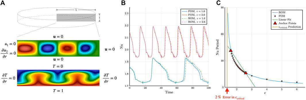
FIGURE 1. ROM application to axisymmetric Rayleigh–Bénard.
While pMOR is a promising approach for engineering analysis and design, it is well known that even the reproduction problem is challenging for the classical POD-Galerkin approach at high Reynolds numbers after the flow transitions to turbulence. One common issue with this class of problems is that the ROM solution approaches an unphysical attractor. This behavior is attributed to a lack of dissipation, given that the truncated POD space lacks high-wavenumber modes that are capable of dissipating energy. One can induce additional dissipation by including more modes but the cost is high. The convective tensor reduction requires storage of N3 entries for the advection operator with a corresponding work of 2N3 operations per timestep. While N = 100, with a cost of a two million operations per step and a million words in memory, may be tolerable, N = 400 with a cost of 128 million operations and 64 million words quickly makes pMOR less viable for running on a workstation, which is typically the target for this type of analysis tool.
Existing techniques for addressing the computational cost include the discrete empirical interpolation method (DEIM) [4], which effectively interpolates the convective term, and tensor decomposition, which aims to approximate the convective tensor by a low-rank tensor. We will show in our concluding examples that these methods will not, on their own, address the unphysical ROM dynamics. Stabilization of the ROM is critical and is the primary topic of this work. Several stabilization strategies are described in Section 2. The major contribution of this work is the development of a novel augmented-basis method (ABM), in which we add important modes to the standard POD bases. In many cases, the ABM increases both the stability and accuracy of the ROMs at a cost equivalent to standard POD approaches having the same total number of modes.
2 Background
The POD-Galerkin technique in fluid flow emerged from work to identify dominant flow features by [5] Model-reduction using POD modes as basis functions was introduced afterwards, with a comprehensive analysis appearing in a later monograph by [5].
More complex PDEs with non-affine parameter dependencies were addressed by [6] using decomposition of the nonlinearity based on the empirical interpolation method (EIM). In this approach, successive interpolation modes are chosen to eliminate the error between the targeted term in FOM and the ROM at “magic points” designated as points in Ω where the error of the current interpolant (i.e., the approximant of the next mode) is maximal. This method was further extended by [4] with a POD decomposition of the nonlinear term and the choice of points restricted to discrete points produced by the spatial discretization of the PDE, called discrete empirical interpolation method (DEIM). While these methods enable application of pMOR to nonlinear problems the issue of insufficient dissipation and feasible stabilization for the NSE persists.
Due to its approach of treating nonlinear terms, DEIM has the potential to address the high-cost issue of including more modes. DEIM replaces the third-order convective tensor with a collocation-like decomposition at the discrete magic points, which yields a reduction of computational complexity from O(N3) to O(N2). Accounting for the constants, evaluation of advection using DEIM with N = 200 modes would be equivalent to using the full tensor with N = 65. For the same cost, DEIM thus permits the use of a richer approximation space.
To certify that the error in the ROMs that are produced is smaller than the acceptable tolerance, error indicators have been developed based on the residual of the ROM solutions in the full-order model (FOM) space. Error indicators for coercive elliptic PDEs are described by [7]. An a posteriori error indicator for time-dependent NSE is described by [8] which is described as the dual-norm of the residual of the time-averaged momentum equation. This error indicator is evaluated by accumulation of residual contributions from each term in the momentum equation at each time-step. This metric provides an error estimate for time-dependent ROM solutions, while not a strict bound on the error, allows an efficient selection of anchor point selection for pMOR. We do not consider these further here, but they are an important component for efficient pMOR and are discussed in a companion paper [9].
For addressing the issue of stability, several modifications to the original POD Galerkin approach have been proposed [10]. proposed a modification of the POD mode generation in which the H1 inner-product is used to produce the Gramian, rather than L2 inner-product, to emphasize the importance of gradients in the FOM snapshots [11]. introduced Leray regularization in the context of ROM in which the advecting field is smoothed (conveniently, by truncation of the modes in the case of POD-ROM). This regularization enhances the stability property of the dynamical behavior; however, the optimal choice of regularization (e.g., number of modes to truncate or shape of transfer function) is not known a priori.
An alternative stabilization approach, introduced by [8], is to replace the discrete ODE system by a constrained minimization problem at each timestep. During the evolution of the system, the basis coefficients are bound by the minimum and maximum coefficient values observed in the snapshot projection onto the truncated POD space. (If the constraints are inactive, one recovers the standard Galerkin-based trajectory.) With this approach, the ROM tends to stay close to the dynamics of the FOM. A challenge, however, is that this approach requires ad hoc modification of the bounds for parametric values where the FOM snapshots are unavailable. Applications of several of these stabilization techniques may be found in [1].
Methods that address the stability issue by constructing basis functions that satisfy the energy-balance that closely match the POD basis is introduced by [12]. In this work, existing work on stabilizing linear time-invariant (LTI) systems by [13], which seeks optimal combinations of snapshots to produce dynamically stable ROMs, is combined with work by [14], in which the kinetic energy behavior is stabilized by introducing an empirical turbulence closure term in the ROM. In this combined method by Balajewicz, in a preprocessing step, an a priori nonlinear constrained optimization problem is solved that minimizes the difference between the energy captured by the new modes and the energy captured by the POD modes for a given N subject to constraints: the columns of the transformation matrix are orthonormal and the empirical kinetic energy-balance is satisfied. The result is a set of transformed POD modes that are augmented directly with dissipation modes (also taken as linear combinations of the snapshots). The author demonstrated that this approach offers significant improvement over the standard POD-Galerkin approach for a 2D lid-driven cavity problem and a 2D mixing layer. Also discovered was the fact that by ensuring the kinetic energy-balance is dissipative to an arbitrary degree, the ROM solution becomes stabilized. Thus, by encapsulating the method by this ROM training stage, the amount of appropriate dissipation to be prescribed in the constrained optimization step can be found to produce a stable ROM with mean TKE behavior close to that of the FOM.
Another basis augmentation approach, introduced by [15,16], uses a combination of L2 POD modes and H1 POD modes that are subsets of the originating snapshot set. The idea is to have a small number of L2 POD modes capture the dominant energy-carrying features of the flow while the H1 POD modes (containing small-scale features) provide the necessary dissipation that is not realized by the L2 POD modes alone. The authors successfully applied this augmented basis to 3D turbulent flow in injectors.
In the next section, we introduce a novel augmented basis method, that is designed to address accuracy and stability of ROMs for turbulent flow. Rather than drawing upon the snapshot set, the augmenting vectors are derived from the nonlinear interaction terms that directly influence the time-derivative of the NSE. This augmented basis set does not require extensive training (i.e., ROM-parameter optimization) and can be used within a standard Galerkin-ROM setting.
3 Augmented basis method
To motivate the ABM, we consider the Leray-projected form of the NSE, in which the velocity field evolution is described as:
Here, the pressure has been formally eliminated and its effects are represented by an abstract operator,
For the spectral element method (SEM), we look to find the solution in a finite-dimensional space,
The method of snapshots forms a basis from a linear combination of FOM solution fields (each involving
Assuming that the solution to Eq. 5 exists near t*, we can describe the local temporal behavior through a Taylor-series expansion involving a linear combination of all time-derivatives.
Therefore, in addition to capturing the dominant modes of the snapshots, we propose to augment the POD basis set ZN with modes that can accurately represent the order ϵ terms on the right-hand side of (7) in order to construct u (x, t* + ϵ). The consequence of not representing the O(ϵ) term is deviation in the trajectory of the physical solution and the projected (Galerkin) solution.
Consider a solution u that lives in ZN, meaning
Thus, we can accurately describe the time-derivative with (N + 1)2 terms for the nonlinear term and (N + 1) terms for the viscous operator.
We consider an example with Fourier basis to highlight this issue. When we have a band-limited solution state with the highest wavenumber k, the convection term would produce a solution at the next timestep of highest wavenumber 2k, which does not live in the original space. Thus, the wavenumber 2k behavior is never observed in the evolution of the projected Galerkin system. With an augmentation of the basis with the high-wavenumber modes, we will face the same issue through lack of 4k mode representation. This issue is of course recursive. We are helped, however, by the fact that the higher wavenumber modes have higher rates of dissipation. Continuation of this process will therefore eventually yield only marginal returns in improved solution fidelity. We shall see, however, that addition of just a few modes can have a significant impact on the overall ROM performance.
Because of nonlinear advection, the solution will evolve outside the N-dimensional span of ZN. We note that as the basis includes more fine-scale components, the convective contribution becomes small relative to the diffusive contribution; thus, the solution becomes closed as the minimal grid-size approaches 0, as is the case in FOM solvers (i.e., the exact solution is band-limited). In the POD-ROM, however, the basis is typically far from completing the relevant approximation space and the addition of the modes
For advection dominated problems, we can focus on the nonlinear contributions,
Whenever we evolve the solution in the space Y, where the current solution lies in the truncated POD space ZN, we see that the time derivative be reasonably represented with an additional (N + 1)2 basis functions of the form
The first subset captures the interaction between the lifting function, ζ0, and all other modes. This choice ensures that both the Taylor dispersion induced by the lifting function and the transport of the mean momentum by the POD modes are accurately captured. This choice is also rationalized by the fact that the lifting function is ever-present in the solution so its convective interaction is important in accurate reproduction of the time-evolution by the ROM. Thus, we add the modes
Next, we extract the diagonal entries,
For a thermal system with an advection-diffusion equation to describe its state, we can follow the same procedure as above for the lifting function interaction in the form of ζ0 ⋅∇θj; however, the auto-interaction modes are not obvious. For this work, we will choose ζj ⋅∇θj, but there is no one-to-one correspondence between the dominant thermal modes and dominant velocity modes. One may come up with a more coherent substitute, but this choice remains an open question.
We note that ABM modes are not orthogonal in general, but are made orthogonal prior to running the ROM via eigendecomposition of the ROM mass matrix for numerical stability purposes. Disregarding round-off errors, the basis representation for a specific solution and test space do not affect the time-evolution of the solution for the standard POD-Galerkin ROM.
In summary, the ABM starts with N standard POD modes in ZN and adds 2N + 1 modes corresponding to advection by the lifting function,
4 Applications
We have demonstrated the effectiveness of the proposed augmentation method on several examples, including flow in a 2D Lid-Driven cavity (Re = 30, 000), 2D flow past baffles (Re = 800), 3D lid-driven cavity flow (Re = 10,000), flow over a hemisphere (Re = 2, 000), and turbulent pipe flow with forced convection for Re = 4,000 −10,000. For brevity, we here consider only the latter two. We will also use the 2D flow past a cylinder problem to demonstrate long-time stable ROM solutions by use of ABM. In the following, we denote the FOM solution with
4.1 2D flow over a circular cylinder
Before we compare the stabilization properties of ABM to other methods, we first investigate the long-time stability properties of ABM on the flow past a cylinder problem. Although this is a canonical problem that is used to demonstrate the model-order reduction capabilities of the POD-Galerkin approach, there are commonly observed instability issues for a large domain. This phenomenon is documented in [19–22]. To establish that ABM addresses this long-time stability issue observed in ROMs of low Reynolds number cylinder flows, we first take 200 snapshots of a flow past a cylinder problem over 200 CTUs. The domain and boundary conditions are of that specified in [20]. Figure 2 shows a velocity magnitude plot of a snapshot used to produce the ROMs.
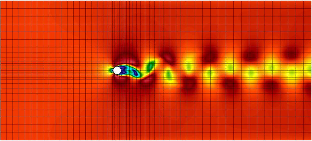
FIGURE 2. Velocity magnitude plot of a flow past a cylinder snapshot (Re = 100)
Figure 3 show reproduction of the 10 mode results in [20] with a difference in the ordering and signs of the POD modes stemming from the difference in snapshot count, snapshot timing, and possibly integration time for the mean flow which is used as the lifting function. For this problem, even if we increase the number of POD modes to N = 20, the growth of the instability is delayed, but is still present in the long-time solution as shown in Figure 4. Application of ABM to 10 originating POD modes resulting in a
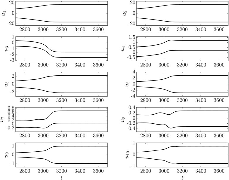
FIGURE 3. POD-ROM coefficient envelopes for flow past a cylinder (N = 10, t ∈ [2,700, 3,700], Re = 100)

FIGURE 4. POD-ROM coefficient envelopes for flow past a cylinder (N = 20, t ∈ [0, 104], Re = 100)
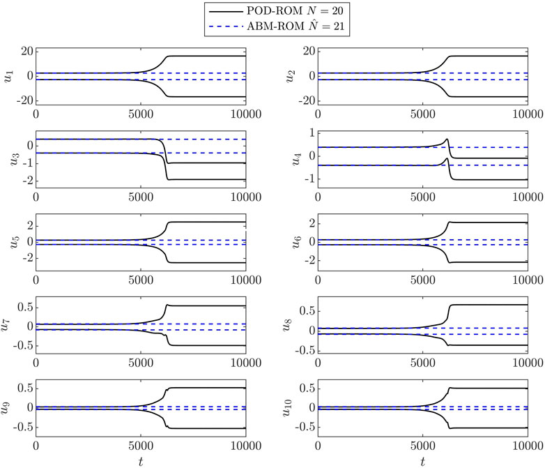
FIGURE 5. ABM-ROM coefficient envelopes for flow past a cylinder (t ∈ [0, 2 × 10⁴], Re = 100)
With this example, we have demonstrated that ABM successfully address long-time stability issue observed in the low-dimensional models constructed by the POD-Galerkin methodology for the cylinder problem. In the next examples, we will show successful application of ABM to 3D turbulence problems.
4.2 3D flow over a hemisphere
Figure 6 shows a snapshot of flow past a wall-mounted hemisphere of height D/2 at ReD = DU/ν = 2000. A Blasius profile with boundary-layer thickness δ99 = 0.6D is prescribed at the inlet, which 3.2D units upstream of the hemisphere center. Periodic boundary conditions are prescribed at ± 3.2D units in the spanwise direction and a stress-free condition is applied on the top surface, 3.2D units above the wall. Under these conditions, the flow exhibits periodic shedding of hairpin vortices, evidenced by the velocity distribution and λ2 contours [23] in the hemisphere wake. The FOM, based on a spectral element mesh with
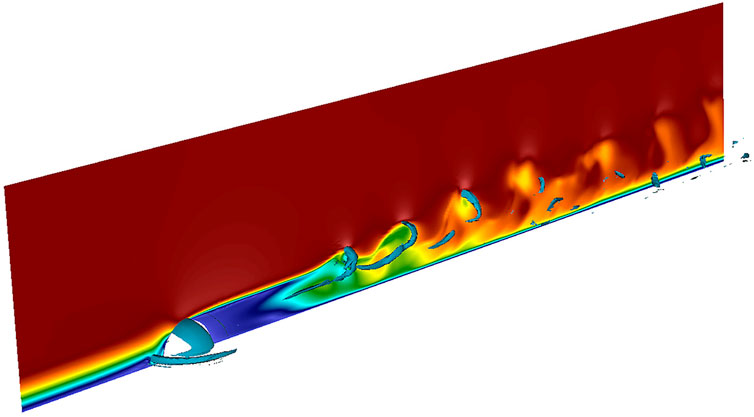
FIGURE 6. FOM velocity magnitude snapshot of flow over hemisphere (Re = 2,000) with overlaid λ2 contour.
The mean-velocity error as a function of
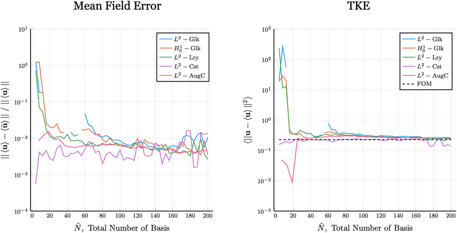
FIGURE 7. Flow over hemisphere (Re = 2,000): Mean and TKE error comparison, curve broken by blowup solution.
4.3 Forced convection in turbulent pipe flow
The next example is that of forced convection in turbulent pipe flow with Reynolds number Re = 4,000, 5300, and 10,000 (based on pipe diameter), and Prandtl number Pr = 1. All the cases use the same spectral element distribution with differing polynomial orders. The mesh consists of 12.5 million grid points for Re = 4,000 and 5300, and 24.5 million points for Re = 10,000. The periodic domain length is L = 4D, which is generally inadequate for a full DNS of turbulence but deemed sufficient for the numerical tests in this study. For Re = 4,000, 5300, and 10,000, the respective FOM Nusselt numbers are Nu = 16.38, 21.42, and 36.14, which is in good agreement with the Dittus-Boelter relationship, Nu = 0.023 Re4/5 Pr2/5. For all cases, the FOM is run until the solution is relaxed to a statistically steady state prior to gathering statistics or snapshot data. For each case, 1,000 snapshots are collected over 50 CTUs to form the Gramian, from which the POD basis is generated. Figure 8 shows typical snapshots of velocity magnitude and temperature that reveal the variation in range of scales for the different cases.
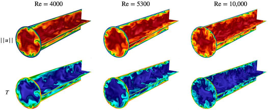
FIGURE 8. FOM velocity (top) and temperature (bottom) snapshots of 3D pipe flow at Re = 4,000, 5300, and 10,000.
The governing equations for the FOM are the incompressible Navier–Stokes equations and the thermal advection-diffusion equation. Because of the constant-flow rate and periodic restriction on the solutions, we provide a brief discussion of modifications to the standard equations for the FOM and their effect on the ROM formulation. We start with the Navier–Stokes equations:
Here, f(u) is a uniform forcing vector field function in the streamwise direction,
Thus, the forcing term in the ROM formulation is zero.
The boundary conditions for the thermal problem are prescribed unit thermal flux on the walls. Therefore, we add a constant-slope ramp function γz such that the lifted temperature T, can be periodic in the domain. The equation becomes
To ensure that thermal energy is conserved in the domain we set
The results for the ROMs are presented in Figures 9–11, which show the error and variance for the velocity and temperature as well as the Nusselt number behavior as a function of the total number of modes. The mean Nusselt number definition is based on the time-averaged streamwise velocity and temperature,
The legends are ordered in the following manner: L2 basis,
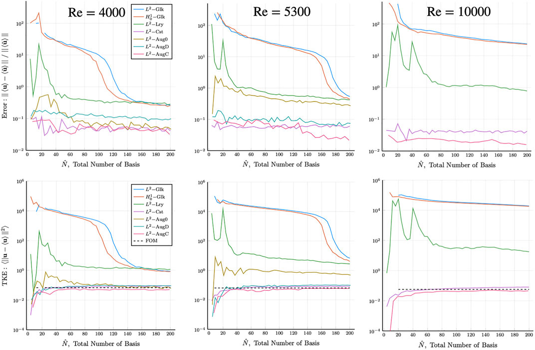
FIGURE 9. Pipe flow mean velocity error (top) and TKE results (bottom), for Re = 4,000, 5300, and 10,000 (FOM: τ = 50, ROM: τ = 500), curve broken by blowup solution.
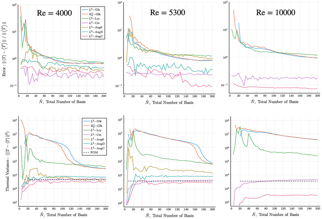
FIGURE 10. Pipe flow mean temperature error (top) and thermal variance results (bottom), for Re = 4,000, 5300, and 10,000 (FOM: τ = 50, ROM: τ = 500), curve broken by blowup solution.
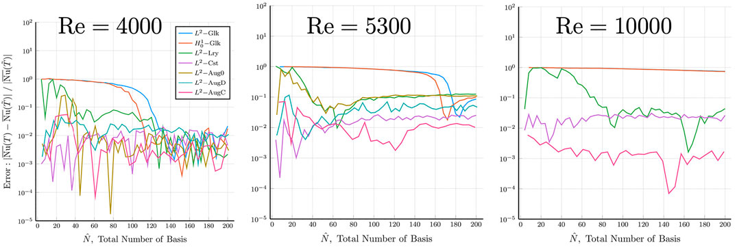
FIGURE 11. Pipe flow error in Nusselt number for Re = 4,000, 5300, and 10,000.
A common observation for Figures 9–11 is nominal convergence for the Re = 4,000 case for the L2,
We close this section with a remark about DEIM as a possible alternative to ABM. Although DEIM allows for larger number of modes in the ROM for a given cost, its accuracy will not surpass that of the underlying ROM formulation on which it is based. So, for a classic L2– or H1–based formulation, DEIM will not yield an acceptable reconstruction result even at N = 200, whereas the constrained and ABM formulations realize convergence at much lower values of
5 Discussion
The ABM has been remarkably successful in advancing our ability to apply ROMs to high-Reynolds number flows. Several observations point to the stabilization properties of the ABM, rather than its approximation quality, as the principal driver for its success. Inspection of the modes for several cases indicate that the augmenting modes in the ABM have high wavenumber content that is localized in Ω to regions of active flow dynamics. An example is illustrated in Figure 12, which shows the first 14 L2–AugC modes for the case of a lid-driven cavity at Re = 30, 000. For j = 0, … , 4, the first five POD modes, ζj ∈ ZN, are in the top row; the first five 0-modes,
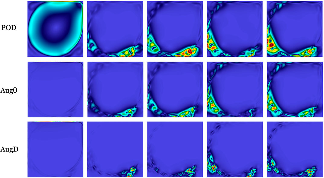
FIGURE 12. Magnitude of POD and ABM modes for a regularized lid-driven cavity problem.
This stabilization hypothesis is supported by the graphs of Figure 13, which shows the amplitudes of the basis coefficients for POD and ABM Galerkin ROM solutions to pipe flow at Re = 5300 as a function of time and mode number. The coefficient evolutions are shown over three time windows [0, 10] [0, 100], and [0, 500], which reveal the growth and saturation of the amplitudes. We see that for the ABM (in the lowest row), the coefficients are all smaller than unity, save for the ζ0 coefficient, which is unity (All modes have unit 2-norm, so the coefficients represent the true amplitude of each scaled mode.) The ABM results also show that most of the energy is in the POD bases, corresponding roughly to the lower third of the mode indices. By contrast, the coefficients for the standard POD Galerkin modes (top row) quickly saturate to amplitudes in excess of 100, and all modes are excited. As is well known from under-resolved Navier-Stokes simulations, there is an energy pile up—manifest as high amplitude modal coefficients—when the representation lacks high wavenumber bases capable of dissipating energy. The Leray-regularized coefficients (second row) exhibit a behavior similar to the standard Galerkin approach, save that the coefficients are much more controlled, which peak amplitudes much closer to unity. The constrained approach (third row) also exhibits chaotic coefficient behavior but at much more controlled amplitudes than either the standard or Leray cases. Remarkably, the evolution on the t = [0, 100] window indicates that the ABM coefficient behavior is nearly time periodic.
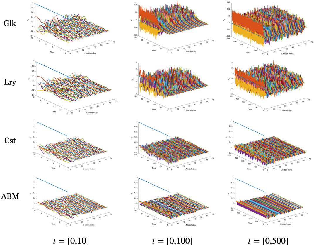
FIGURE 13. Temporal behavior of basis coefficients for standard POD (Glk), Leray-filtered (Lry), Constrained (Cst), and ABM-ROM solutions of turbulent pipe flow at Re = 5300 over (convective) time intervals t ∈ [0, 10] [0.100], and [0.500].
Another study to investigate the role of dissipation is illustrated in Figure 14. We focus initially on the upper left graph, which shows the mean-flow error for the standard POD-ROM case as a function of the number of modes
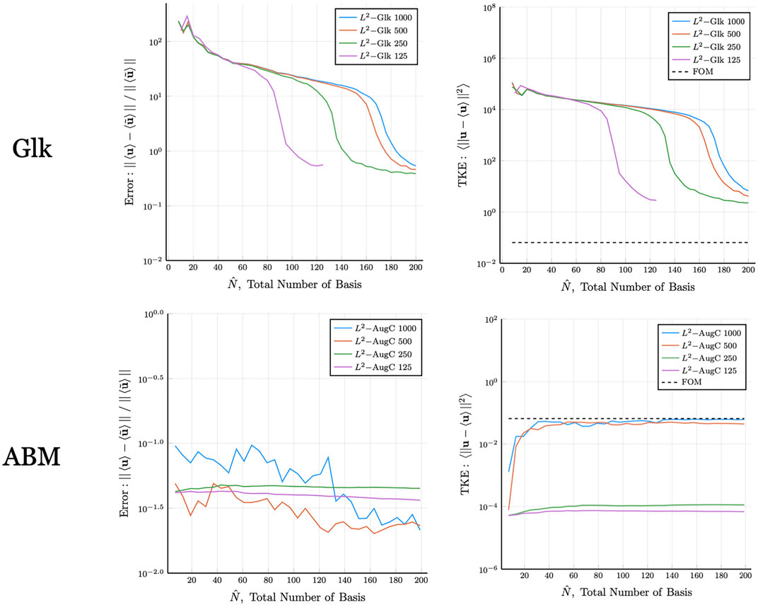
FIGURE 14. Convergence for mean velocity (left) and TKE (right) for turbulent pipe flow at Re = 5300 as a function of the number of modes for the POD-ROM (top) and ABM-ROM (bottom). The dimension of the snapshot space, K, is indicated in the legend.
The effectiveness of the ABM approach in a pMOR context is demonstrated by considering the pipe flow problem with two sets of snapshots at Re = 5300 and Re = 10,000. Combining 1,000 snapshots from each anchor point, we obtain 30 POD modes and 61 ABM modes using the average of the mean velocity solutions at the anchor points as the lifting function. Running this ROM for Re ∈ {4,000, 5000, … , 10,000} resulted in a parameteric behavior that is consistent with the physical flow: as Reynolds number is increased, the boundary layer thickness decreases according to the law of the wall and the turbulence fluctuation adjacent to the wall region increases. Figure 15 depict the mean axial flow profile. This profile was produced by an additional spatial averaging in the axial and azimuthal directions. More detailed analysis will be conducted in the future, but this preliminary example pMOR application provides evidence that ABM-ROM is a promising approach for pMOR of turbulent flows.

FIGURE 15. Time- and space-averaged axial velocity profiles for ABM-ROM pMOR.
6 Conclusion
We introduced a novel stabilization method, ABM, for ROM-based simulations of incompressible turbulent flows that augments the standard POD basis with approximate temporal derivatives. For a space of POD basis functions, ZN = {ζi}, i = 0, … , N, we include and additional 2N + 1 functions that are the Leray (divergence-free) projections of the nonlinear interactions with the lifting mode, {ζ0 ⋅∇ζi + ζi ⋅∇ζ0}, and nonlinear auto-interactions, {ζi ⋅∇ζi}. With these basis functions, the ROM proceeds in the standard Galerkin fashion and is seen to dramatically outperform standard L2-and
We showed that the auxiliary modes of the ABM have high wavenumber content that is localized to regions in Ω where flow gradients are large and thus provide efficient dissipation mechanisms that are lacking in standard POD bases. We further demonstrated that, for standard POD methods, having a more complete POD space (i.e., incorporating N ≈ K modes from a relatively small snapshot space of rank K) yields lower errors than having N′ > N POD modes from a larger snapshot space of rank K′ > N′. The reasoning is the same—the more complete space includes high wavenumber content in the ROM basis set that provides dissipation and hence stability. Analysis of the ROM coefficient time-traces for turbulent pipe flow at Re = 5300, illustrated that the amplitudes of all the modes for non-stabilized POD-ROM are orders of magnitude larger than their stabilized counterparts. While Leray-based stabilization mitigates this behavior, it still yields coefficient amplitudes that are roughly a factor of ten greater than observed in either the constrained or ABM-based formulations.
The ABM was also shown to be effective for predicting thermal QOIs such as Nusselt numbers. It was, however, a bit overly dissipative at Re = 10, 000. The study of the interplay between N and K indicates that this dissipation can be controlled with these two parameters and one might therefore use these parameters to gain insight to the root cause of the over-dissipation. Future work will include application of the ABM to higher Reynolds number flows and to more complex domains.
Data availability statement
The original contributions presented in the study are included in the article/Supplementary Materials, further inquiries can be directed to the corresponding author.
Author contributions
Research was performed by KK under advisement and direction of PF. The two authors both contributed to the production of the manuscript.
Funding
This work from NEUP with number DE NE0008780 for Turbulent Heat-Transfer ROM research was used. This research is supported by the DOE Office of Nuclear Energy under the Nuclear Energy University Program (Proj. No. DE_NE0008780). The research used resources at the Oak Ridge Leadership Computing Facility at Oak Ridge National Laboratory, which is supported by the Office of Science of the U.S. Department of Energy under Contract DE-AC05-00OR22725 and at the Argonne Leadership Computing Facility, under Contract DE- AC02-06CH11357.
Conflict of interest
The authors declare that the research was conducted in the absence of any commercial or financial relationships that could be construed as a potential conflict of interest.
Publisher’s note
All claims expressed in this article are solely those of the authors and do not necessarily represent those of their affiliated organizations, or those of the publisher, the editors and the reviewers. Any product that may be evaluated in this article, or claim that may be made by its manufacturer, is not guaranteed or endorsed by the publisher.
Footnotes
1These equations are effectively in nondimensional form, which for forced conditions implies that ν = Re−1, the inverse Reynolds number, and α = Pe−1, the inverse Peclet number. For buoyancy-driven flows these parameters typically scale with Rayleigh number (Ra) and Prandtl number (Pr), with the precise definition dependent on the chosen scaling.
References
1. Kaneko K, Tsai P-H, Fischer P. Towards model order reduction for fluid-thermal analysis. Nucl Eng Des (2020) 370:110866. doi:10.1016/j.nucengdes.2020.110866
2. Tuckerman L, Barkley D. Global bifurcation to traveling waves in axisymmetric convection. Phys Rev Lett (1988) 61:408–11. doi:10.1103/physrevlett.61.408
3. Barkley D, Tuckerman L. Traveling waves in axisymmetric convection: The role of sidewall conductivity (1989).
4. Chaturantabut S, Sorensen DC. Nonlinear model reduction via discrete empirical interpolation. SIAM J Scientific Comput (2010) 32:2737–64. 10.1137/090766498.(Accessed March 26, 2022)
5. Holmes P, Lumley JL, Berkooz G. Turbulence, coherent structure, dynamical systems and symmetry. Cambridge University Press (1996). doi:10.1017/CBO9780511622700
6. Barrault M, Maday Y, Nguyen N, Patera A. An ‘empirical interpolation’ method: Application to efficient reduced-basis discretization of partial differential equations. C R Math (2004) 339:667–72. doi:10.1016/j.crma.2004.08.006
7. Veroy K, Rovas DV, Patera A. A posteriori Error estimation for reduced-basis approximation of parametrized elliptic coercive partial differential equations: “Convex inverse” bound conditioners. convex inverse” bound conditioners (2002) 8:1007–28. doi:10.1051/cocv:2002041
8. Fick LH, Maday Y, Patera AT, Taddei T. A stabilized POD model for turbulent flows over a range of Reynolds numbers: Optimal parameter sampling and constrained projection. J Comput Phys (2018) 371:214–43. doi:10.1016/j.jcp.2018.05.027
9. Tsai P-H, Fischer P. Parametric model-order-reduction development for unsteady convection. Front Phys (2022).
10. Iollo A, Lanteri S, Desideri JA. Stability properties of POD-galerkin approximations for the compressible Navier-Stokes equations. Theor Comput Fluid Dyn (2000) 13:377–96. doi:10.1007/s001620050119
11. Wells D, Wang Z, Xie X, Iliescu T. An evolve-then-filter regularized reduced order model for convection-dominated flows. Int J Numer Methods Fluids (2017) 84:598–615. doi:10.1002/fld.4363
12. Balajewicz M. A new approach to model order reduction of the Navier-Stokes equations. Durham, NC: Duke University (2012). Ph.D. thesis.
13. Amsallem D, Farhat C. Stabilization of projection-based reduced-order models. Int J Numer Methods Eng (2012) 91:358–77. doi:10.1002/nme.4274
14. Cazemier W, Verstappen RWCP, Veldman AEP. Proper orthogonal decomposition and low-dimensional models for driven cavity flows. Phys Fluids (1998) 10:1685–99. doi:10.1063/1.869686
15. Akkari N, Mercier R, Lartigue G, Moureau V (2017). Stable POD-Galerkin Reduced Order Models for unsteady turbulent incompressible flows. In 55th AIAA Aerospace Sciences Meeting (Grapevine, United States)
16. Akkari N, Casenave F, Moureau V. Time stable reduced order modeling by an enhanced reduced order basis of the turbulent and incompressible 3d Navier–Stokes equations. Math Comput Appl (2019) 24:45. doi:10.3390/mca24020045
17. Fischer P. An overlapping schwarz method for spectral element solution of the incompressible Navier–Stokes equations. J Comput Phys (1997) 133:84–101. doi:10.1006/jcph.1997.5651
18. Sirovich L. Turbulence and the dynamics of coherent structures. I. Coherent structures. Q Appl Math (1987) 45:561–71. doi:10.1090/qam/910462
19. Noack BR, Afanasiev K, Morzyński M, Tadmor G, Thiele F. A hierarchy of low-dimensional models for the transient and post-transient cylinder wake. J Fluid Mech (2003) 497:S0022112003006694–363. doi:10.1017/s0022112003006694
20. Sirisup S, Karniadakis GE. A spectral viscosity method for correcting the long-term behavior of pod models. J Comput Phys (2004) 194:92–116. doi:10.1016/j.jcp.2003.08.021
21. Akhtar I, Nayfeh AH, Ribbens CJ. On the stability and extension of reduced-order galerkin models in incompressible flows. Theor Comput Fluid Dyn (2009) 23:213–37. doi:10.1007/s00162-009-0112-y
22. Hay A, Borggaard J, Akhtar I, Pelletier D. Reduced-order models for parameter dependent geometries based on shape sensitivity analysis. J Comput Phys (2010) 229:1327–52. doi:10.1016/j.jcp.2009.10.033
Keywords: POD, ROM, pMOR, stabilization, turbulence
Citation: Kaneko K and Fischer P (2022) Augmented reduced order models for turbulence. Front. Phys. 10:905392. doi: 10.3389/fphy.2022.905392
Received: 27 March 2022; Accepted: 05 August 2022;
Published: 29 September 2022.
Edited by:
Traian Iliescu, Virginia Tech, United StatesReviewed by:
Imran Akhtar, National University of Sciences and Technology (NUST), PakistanBirgul Koc, Sevilla University, Spain
Copyright © 2022 Kaneko and Fischer. This is an open-access article distributed under the terms of the Creative Commons Attribution License (CC BY). The use, distribution or reproduction in other forums is permitted, provided the original author(s) and the copyright owner(s) are credited and that the original publication in this journal is cited, in accordance with accepted academic practice. No use, distribution or reproduction is permitted which does not comply with these terms.
*Correspondence: Kento Kaneko, a2FuZWtvMkBpbGxpbm9pcy5lZHU=