 Cheng Huang
 Karthik Duraisamy
 Charles Merkle
- 1Department of Aerospace Engineering, University of Kansas, Lawrence, KS, United States
- 2Department of Aerospace Engineering, University of Michigan, Ann Arbor, MI, United States
- 3School of Aeronautics and Astronautics, Purdue University, West Lafayette, IN, United States
Large-scale engineering systems, such as propulsive engines, ship structures, and wind farms, feature complex, multi-scale interactions between multiple physical phenomena. Characterizing the operation and performance of such systems requires detailed computational models. Even with advances in modern computational capabilities, however, high-fidelity (e.g., large eddy) simulations of such a system remain out of reach. In this work, we develop a reduced‐order modeling framework to enable accurate predictions of large-scale systems. We target engineering systems which are difficult to simulate at a high-enough level of fidelity, but are decomposable into different components. These components can be modeled using a combination of strategies, such as reduced-order models (ROM) or reduced-fidelity full-order models (RF-FOM). Component-based training strategies are developed to construct ROMs for each individual component. These ROMs are then integrated to represent the full system. Notably, this approach only requires high-fidelity simulations of a much smaller computational domain. System-level responses are mimicked via external boundary forcing during training. Model reduction is accomplished using model-form preserving least-squares projections with variable transformation (MP-LSVT) (Huang et al., Journal of Computational Physics, 2022, 448: 110742). Predictive capabilities are greatly enhanced by developing adaptive bases which are locally linear in time. The trained ROMs are then coupled and integrated into the framework to model the full large-scale system. We apply the methodology to extremely complex flow physics involving combustion dynamics. With the use of the adaptive basis, the framework is demonstrated to accurately predict local pressure oscillations, time-averaged and RMS fields of target state variables, even with geometric changes.
1 Introduction
Rapid advancements in computing technologies are enabling high-fidelity simulations of complex, multi-scale physics (e.g., turbulence [1] and combustion [2,3]) observed in real engineering systems. These simulations provide insight into the underlying physics, which cannot be quantitatively accessed through experiments. This insight is useful in improving the performance of engineering systems and reducing failures. However, the high computational costs of high-fidelity simulations prohibit their integration into design and analysis of full-scale systems, which require repeated simulations to explore parameter spaces. One popular approach to address such challenges is through model order reduction (MOR), a common approach being projection-based reduced-order models (ROM) [4–6], which have demonstrated success in many applications such as flow control [7–9], aeroelasticity [10,11], hypersonics [12], and combustion [13,14]. Typically, the construction of ROMs involves three stages: 1) an offline training stage that performs high-fidelity simulations of the target systems for multiple parameters; 2) offline construction of reduced basis and projections on low-dimensional manifolds; and 3) online execution of ROMs by projecting the governing equations on the low-dimensional manifold. Despite the many successful examples of MOR, their direct applications in many practical large-scale engineering systems remain infeasible because the systems are so complex that high-fidelity simulations are completely inaccessible. Using an example from rocket combustion, a coarse-mesh (“low”-fidelity) large eddy simulation (LES) of a small-scale rocket engine [15] requires O(107) CPU-hours, which even makes a single fine-mesh (high-fidelity) LES of this type of problems inaccessible, (estimated to require
To address this specific challenge of the lack of full-order model (FOM) data for large-scale systems, researchers have formulated domain-decomposition methods [17,18], or component-based methods [19] to develop a network of ROMs to model the target system. In addition to ROM applications, such ideas have been commonly used for computational fluid dynamics [20,21], port-hamiltonian system [22–24] etc. For consistency, we refer to this family of approaches as component-based reduced-order modeling (CBROM) methods in the current paper. CBROM methods leverage the fact that many large-scale engineering systems can be decomposed into components of identical features and the offline training of the ROMs can be performed based on each individual component for multiple parameters, which significantly reduces the cost of the offline training. The trained component-based ROMs can then be used for the identical components and coupled together to model different configurations of the large-scale systems.
To date, the majority of the success of CBROM methods has been in problems governed by linear PDEs. Willcox et al. [25] demonstrated the feasibility of constructing low-order models of blade row unsteady aerodynamics in a compressor. Maday and Ronquist [26] formulated a reduced basis element method and applied it to a thermal fin problem. Iapichino et al. [27] proposed a reduced basis hybrid method to solve the steady Stokes problem with applications to cardiovascular networks. Adopting the static-condensation reduced-basis-element method [19,28,29], Kapteyn et al. [30] demonstrated the development of a digital twin for a 12-ft wingspan unmanned aerial vehicle via a library of component-based ROMs. More recently, McBane and Choi [31] leveraged the static-condensation reduced-basis-element method and demonstrated a 1000× speedup with relative error
In addition, some applications of component-based ROMs on nonlinear PDEs can also be found in the literature. One group of studies incorporate the FOM to model a subset of components in the target system while applying ROMs to the other components. Lucia et al. [32] demonstrated a combination of ROMs and FOM by domain-decomposition for modeling two-dimensional high-speed flows with moving shock waves, by applying the FOM for the shock-containing domain and ROMs for the other domains. Buffoni et al. [33] demonstrated similar ideas by partitioning the computational domain into two subdomains (one modeled using FOM while the other by ROM), and presented different approaches to couple ROM with FOM. Baiges et al. [34] demonstrated the improvement in predicting flow configurations that are not present in the training snapshots by integrating the FOM into the component-based modeling framework. Ahmed et al. [35] presented a hybrid analysis and modeling approach combining a physics-based FOM and a data-driven non-intrusive ROM towards predictive digital twin technologies. Another group of investigations aim at incorporating only ROMs rather than hybrid FOMs/ROMs in the component-based modeling framework. Hoang et al. [36] proposed the domain-decomposition least-squares Petrov-Galerkin (DD-LSPG) model-reduction method for parameterized systems of nonlinear algebraic equations. Xiao et al. [37–39] developed a domain-decomposition non-intrusive reduced-order model (DDNIROM) for turbulent flows. The current authors demonstrated the integration of component-based ROMs with a FOM in a quasi-1D Euler problem [40,41].
In the present work, we develop a component-based modeling framework that can flexibly adopt either reduced-order models (ROM) or full-order models (FOM) for different components of the target system based on the corresponding requirements of modeling accuracy and efficiency with the goal of enabling:
(1) Accurate simulations of large-scale systems, which cannot be directly accessed using high-fidelity simulations;
(2) Parametric studies of the large-scale system targeting many-query applications.
It is notable that in the current work, we choose rocket engine as the target system. This application involves compressible, reacting, chaotic flows and thus introduces complex challenges for reduced order modeling. We establish a component-based training strategy for ROM development, which only requires the high-fidelity simulations of the individual components, rather than the entire system. The trained ROMs are then coupled together (either with each other or with FOM) via a direct flux matching method for information transfer between components. The ROM formulation leverages model reduction techniques using model-form preserving least-squares projections with variable transformation (MP-LSVT) with physical realizability enforced on both temperature and species mass fractions [14] to achieve both global and local stabilization. Furthermore, the MP-LSVT ROM is incorporated with basis adaptation to achieve significant enhancement in modeling accuracy. Since our interests are focused on engineering systems involving combustion, we use extremely challenging turbulent reacting flow examples, relevant to rocket applications, to motivate and evaluate our framework. But it should be highlighted that our component-based modeling framework is applicable to many other, unrelated disciplines, featuring systems that can be decomposed into different components.
The remainder of the paper is organized as follows. Section 2 presents the full-order model (FOM) and time discretization. Section 3 reviews the procedure for model reduction via MP-LSVT formulation. Section 4 discusses basis-adaptation algorithms for ROM enhancement. Section 5 presents the domain-decomposition framework, including both the component-based ROM training strategy and integration method in full system. Section 6 presents numerical results based on single- and multi-injector model rocket combustor configurations with detailed assessment on the accuracy of the framework. In Section 7, we provide concluding remarks and perspectives.
2 Full-Order Model
We define the physical domain Ω with boundary ∂Ω, and then represent the governing equations of the full-order model (FOM) for Ω as a generic dynamical system
where t ∈ [0, T] is the solution time, which spans the time interval from 0 to T,
Different time-discretization methods can be introduced to solve Eq. 1 (e.g., linear multi-step, or Runge–Kutta methods [42]). For all the numerical examples presented in the current paper, we use linear multi-step methods for both FOM and ROM calculations and refer the reader to [14] for details. An l-step version of linear multi-step methods can be expressed as
where
3 Model-Form Preserving Model Reduction for Transformed Solution Variables
For problems involving multiscale phenomena with strong convection and non-linear effects, it is well-recognized that ROM robustness can be a major issue. To address this challenge, we pursue the model-form preserving least-squares with variable transformation (MP-LSVT) formulation to construct the reduced-order model (ROM). This methodology is described below—we refer the reader to ref [14] for further details.
3.1 Construction of Proper Orthogonal Decomposition Bases for Solution Variables
The state qp in Eq. 1 can be expressed in a trial space
where
where Q is a data matrix in which each column is a snapshot of the solution
where
3.2 Least-Squares With Variable Transformation
Leveraging the least-squares Petrov-Galerkin (LSPG) projection formulation proposed by Carlberg et al. [43], we develop a model-form preserving least-squares formulation for the FOM in Eq. 1. Our objective is to minimize the fully-discrete FOM equation residual r, defined in Eq. 2, on the physical domain Ω with respect to the reduced state, qr
where the approximate solution variables,
where
such that each equation in r has similar contributions to the minimization problem in Eq. 7. It is worth pointing out that the treatment of boundary conditions in the MP-LSVT ROM is fully consistent with the FOM in Eq. 2, which guarantees that the boundary conditions are satisfied in the ROM and serves as an important building block in FOM/ROM coupling in the component-based domain-decomposition framework in Section 5.
Following Eq. 7, a reduced non-linear system of dimension np can then be obtained and viewed as the result of a Petrov-Galerkin projection
where Wp is the test basis
with
4 Reduced-Order Models Enhancement via Basis Adaptation
While the MP-LSVT method improves the robustness and accuracy of the ROM, predictive capabilities (e.g., future-state prediction) are still restricted by the use of linear static basis, which has been shown to be inadequate for predictions in problems with slow Kolmogorov N-width decay [14,44]. Several remedies have been proposed to address this challenge through, for example, localized linear bases [45,46], nonlinear bases [47,48], and online basis adaptation [49–51] etc. In the current work, we focus on online basis-adaption methods, which aim to update the trial basis Vp during the online ROM calculation (Eq. 10) such that
where r is the fully-discrete FOM equation residual defined in Eqs. 2,
where the basis at time-step n − 1 is adapted to n, through an increment,
where
here, we adopt an alternate formulation compared to [50] by updating the basis based on the full-state information evaluated at the current time step, n,
To achieve gains in computational efficiency for the projection-based ROMs introduced in Section 3, hyper-reduction is required to obtain an approximation of the non-linear function (e.g., f in Eq. 1) based on a small number of sampled elements—for example, it can be achieved by the discrete empirical interpolation method (DEIM) [52], or its least-squares regression analogue, gappy POD Everson and Sirovich [53]. In addition, the full-state information evaluation (Eq. 15) in basis adaptation can be computationally expensive and also requires hyper-reduction for efficiency gain so that the evaluation is only needed at a small number of sampled elements. This can be achieved by incorporating the recently developed adaptive sampling techniques [50], which update the selection of sampled elements based on the basis adaptation. However, the current work mainly focuses on the development and demonstration of the component-based ROM framework. Therefore for conciseness, we are not including ROM hyper-reduction in the current paper since in principle, its presence or absence will not impact the validity of the framework. We will incorporate the hyper-reduced ROMs in the framework in future work.
5 Component-Based Domain-Decomposition Framework
In this section, we introduce the component-based domain-decomposition framework for modeling large-scale engineering systems. Because our research has been primarily motivated by applications to propulsion systems for aerospace applications, we use a multi-injector model rocket combustor to assist in the description of the framework formulation. Figure 1 presents a representative geometry composed of seven injector elements through each of which fuel and oxidizer in separate channel feed a downstream combustion chamber. The physical domain has been separated into eight components with seven for the injector elements (Ωk, etc.) and one for the downstream combustor and nozzle (Ω8). A set of similar configurations are also included in our numerical examples in Section 6.2. Even though the configuration in Figure 1 represents a complicated engineering system, most of the components share identical geometric features, an attribute that is common in many engineering systems (e.g., compressors, gas turbine engines, and wind farms, etc.). The interior components Ωk, where k = 2, … , 6, are identical to each other geometrically, the two outer components Ω1 and Ω7 mirror each other in geometrical configuration (i.e., symmetric about the center axis), while Ω8 does not resemble any other components. Therefore, the representation of the multi-injector rocket combustor in Figure 1 can be simplified as the combination of three representative components: I
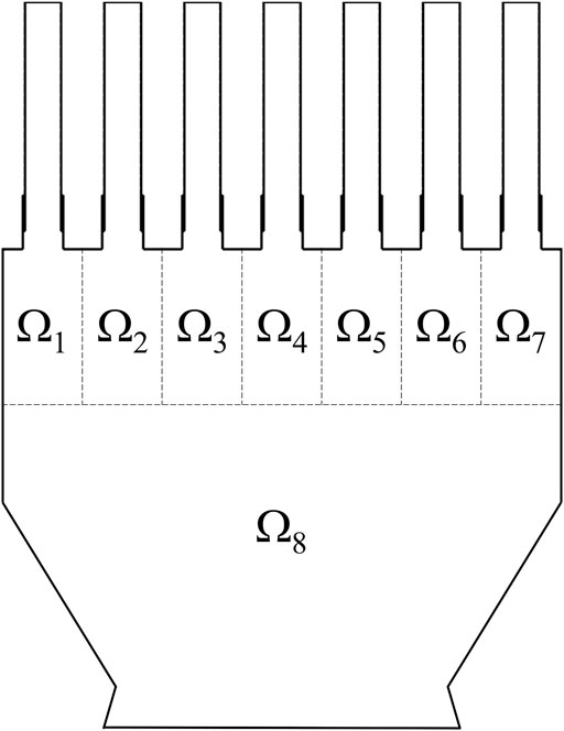
FIGURE 1. An example of a multi-injector model rocket combustor with seven identical injector elements and the downstream combustor and nozzle [54].
First, we introduce a general description of the domain-decomposition formulation
where k denotes the numbering of the sub-components in the formulation,
Given the complexity and scale of the physics, small-scale local components with identical features (e.g., the interior and outer injector elements, Ω3 and Ω7, in Figure 1, the nozzle element in a gas turbine, the rotor blade in a compressor, or the wind turbine in a wind farm) often require high-fidelity modeling to achieve satisfying accuracy in many-query engineering applications. Therefore, ROMs can be an ideal candidate from the viewpoint of satisfying efficiency and accuracy requirements. On the other hand, large-scale system-level components (e.g., the downstream combustor and nozzle, Ω8, in Figure 1) are usually governed by physics that is less demanding in numerical resolution. This makes the reduced-fidelity full-order model (RF-FOM) a good candidate for modeling of the large-scale system-level components—for example, coarse-mesh LES, nonlinear Euler model, unsteady Reynolds Averaged Navier Stokes models.
5.1 Component-Based Reduced-Order Model Training
To enable modeling of the full system (e.g., Figure 1), the FOM of which is not directly accessible, we develop a component-based ROM training method in the current section, that requires high-fidelity FOM simulations for only the reference components identified in the system. The method aims to generate a rich training dataset that contains representative dynamics of the components when integrated in the full system of various configurations (e.g., different numbers of injector elements), thus enabling the generation of predictive component-based ROMs, which is analogous to the localized ROM strategy developed for finite element method with representative work by Henning and Peterseim [56]; Eftang and Patera [28]; and Smetana and Patera [29]. To achieve this, we introduce unsteady perturbations at interface boundaries in the FOM simulations of the reference components, following Eq. 1, to fabricate the effects of system-level responses, as demonstrated in Figure 2. Most importantly, by enriching the functions used for the boundary perturbations, the dynamics of different full-system configurations can be embedded within the ROMs of the individual components. For example, the effects of system-level acoustics can be accounted for by imposing different pressure perturbations at the boundary
where fi is the frequency included in the boundary perturbations with Ai denoting the associated amplitude, reflecting the anticipated full-system responses, and nf is the total number of frequencies, an indicator of the richness of the excited dynamics. Alternatively, velocity oscillations can be enforced at the boundaries following similar function in Eq. 17 to mimic the effects of large-scale flow dynamics in the full system.
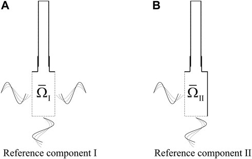
FIGURE 2. Schematic of the component-based ROM training method based on (A) reference components I and (B) II.
It is important to ensure that the imposed boundary conditions (dashed lines in Figure 2) do not imprint the dimensions of the individual component upon the combustion dynamics. All internal domains are subject to acoustic resonance at scales determined by their geometry, but the dimensions in the individual component are not representative of those of the full system and so must not appear in the training dataset. Accordingly, it is critical that the boundary conditions on the reference component be chosen such that its geometry does not impact the FOM solutions of the dynamics upon which the ROM is based. An effective way to accomplish this is by applying non-reflective boundary conditions through pertinent Riemann invariants. We adopt the formulation that proved to be effective for multi-dimensional reacting flow simulations [57]. It should be mentioned that the ROM training method in Figure 2 requires a level of prior knowledge of the essential physics in the full-system (e.g., acoustics) to ensure that pertinent physics are included in the ROM training. For example, in rocket combustor design such as Figure 1, system-level acoustic frequencies can be estimated a priori based on the full-system configuration. Correspondingly, a multi-frequency perturbation can be imposed at the boundary conditions for ROM training, the frequency band of which covers the target full-system acoustic frequencies and therefore excites the essential dynamics anticipated within the component when integrated in the full-system. A similar idea has been demonstrated in simple 1D problems by the current authors Huang et al. [40]; Xu et al. [41]. To account for complex dynamics at the component interfaces, instead of directly imposing the perturbations at the interfaces, auxiliary domains can be introduced for the ROM training, which is discussed and demonstrated in Section 6.
5.2 Integration in Full System Simulations
Once the component-based models are constructed following the strategies in Section 5.1, the effective integration of these models in the domain-decomposition framework is another determining factor for the success of the framework. In this section, we use the example in Figure 1 to illustrate the integration of the component-based models. Following the method in Section 5.1, ROMs are trained on the reference components, the trained ROMs can be used repetitively to model identical components in the full system to enable geometric variations (Figure 3A with
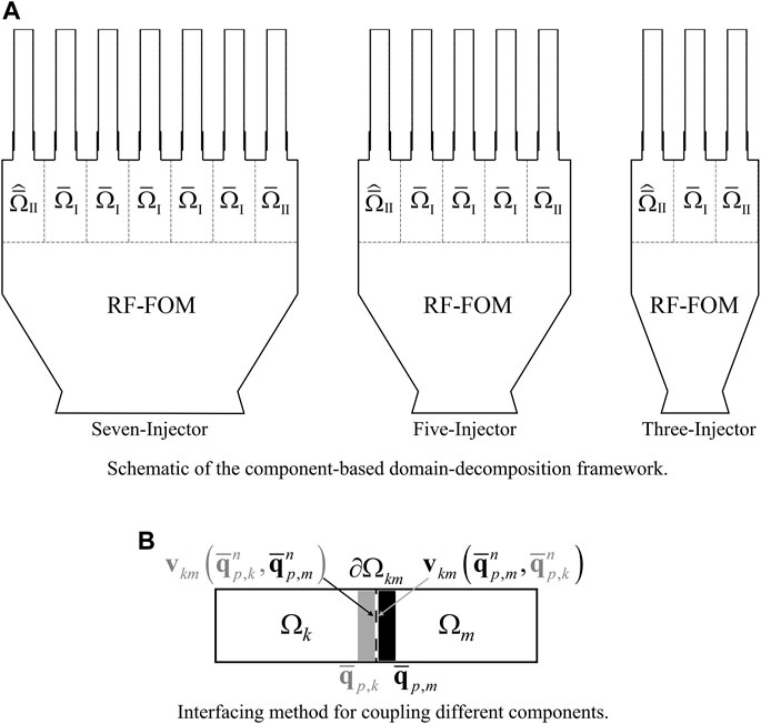
FIGURE 3. Illustration of the component-based domain-decomposition framework. (A) Schematic of the component-based domain-decomposition framework. (B) Interfacing method for coupling different components.
To achieve accurate predictions of the system-level response governed by the component interactions, it is important to ensure that the essential information is transferred between components. We adopt a direct flux matching method via ghost cell assignment to couple the components at the interface with no overlap
a schematic of which is shown in Figure 3B, describing the coupling between domain Ωk and Ωm through the interface ∂Ωkm. The two adjacent mesh cells of ∂Ωkm are indicated by the shaded areas. When performing calculations based on Eq. 16 at time step n at a cell with solution variables
The major benefit of the direct-flux-matching interfacing method is that it inherently accounts for changes in flow characteristics at the interface and therefore important phenomena such as reverse flows are naturally supported. More importantly it makes the training of the component-based ROMs relatively independent of their coupling with other components in the framework, which allows more flexibility in the ROM training strategy. For example, auxiliary domains (e.g., adjacent injector elements) can be introduced in the component-based ROM training stage in Figure 2 to better emulate interactions between injector elements in the training dataset. These aspects are demonstrated in the numerical results in Section 6.
6 Numerical Results
To assess the capabilities of component-based domain-decomposition modeling framework in predicting multi-scale multi-physics problems (e.g., reacting flows), two model rocket combustors are considered. The first configuration is a two-dimensional representation of a generic laboratory-scale single injector configuration [59]. This case is used to a) assess the component-based ROM training strategy and the interfacing method between components in the framework, and b) to explore the feasibility of using the framework to predict dynamics on different full-system geometries. The second configuration is a two-dimensional representation of a multi-injector model rocket combustor [60], and is used to evaluate the capabilities of the framework to model different geometric configurations of the full system as demonstrated in Figure 3.
The computational infrastructure used for the full- and reduced-order models solves conservation equations for mass, momentum, energy and species transport [58,61] in a fully coupled manner, which has been used to model a variety of complex, practical reacting flow problems. More details of the FOM equations can be found in Appendix B of [14]. The FOM employs a cell-centered second-order accurate finite volume method for spatial discretization and uses the direct flux matching method as described in Section 5.2 for parallel computation. The Roe scheme [62] is used to evaluate the inviscid fluxes and a Green-Gauss gradient reconstruction procedure [63] is used to compute the face gradients and viscous fluxes. A gradient limiter by Barth and Jespersen [64] is used to preserve monotonicity for flow fields with strong gradients. A ghost cell formulation is used for treatment of boundary conditions. Time integration for all FOM simulations uses the implicit second-order accurate backwards differentiation formula with dual time-stepping.
6.1 Single-Injector Model Rocket Combustor
First, we explore and demonstrate the component-based domain-decomposition framework on a 2D-planar representation of a generic laboratory-scale rocket combustor designed to study combustion dynamics [59]. The configuration is shown in Figure 4A and consists of a shear coaxial injector with an outer passage, T1, that introduces fuel near the downstream end of the coaxial inner passage, T2, which in turn feeds oxidizer to the combustion chamber with a choked nozzle downstream, resulting in combustion-driven acoustics to be sustained. Operating conditions in this single-injector combustor are maintained with an adiabatic flame temperature of approximately 2,700 K and a mean chamber pressure of 0.95 MPa. The T1 stream contains gaseous methane (100% CH4) at 300 K. The T2 stream is 42% gaseous O2 by mass and 58% gaseous H2O by mass at 660 K. The T1 and T2 streams are maintained at constant mass flow rates, 0.46 kg/s and 5.40 kg/s, respectively. Combustion is represented by the flamelet progress variable (FPV) model [65] with GRI-1.2 [66] chemical kinetics, which consists of 32 species and 177 chemical reactions. The chemical species are treated as thermally perfect gases. Note that although 32 chemical species are modeled, the FPV model only solves transport equations for three scalar quantities: the mean mixture fraction (Zmean), the mixture fraction variance (Z″2), and the reaction progress variable (Cmean) [65]. Individual chemical species mass fractions are looked up from pre-computed flamelet manifolds [67].

FIGURE 4. Overview of 2D-planar single-injector model rocket combustor including (A) computational configuration and FOM-FOM results with (B) pressure signals measured at x = 0 in (A,C) representative snapshots of the temperature fields, and (D) representative snapshots of the axial velocity fields.
As shown in Figure 4A, the single-injector configuration consists of two components, the upstream injector element (ΩA) and the downstream combustor and nozzle (ΩB). Three different lengths of the combustor (Lc) are investigated for this configuration by maintaining the upstream component (ΩA) while varying the length of the downstream component (ΩB), i.e., LB. This change in length leads to different dynamic behaviors as shown in Figures 4B–D when both ΩA and ΩB adopt FOM as their modeling strategy, denoted as FOM-FOM, the solutions from which are taken as the truth to evaluate the component-based ROM framework. It can be readily seen from Figure 4B that by just varying the combustor length (Lc), different pressure oscillations can be sustained. The longer combustor lengths tend to drive higher pressure oscillation amplitudes (
6.1.1 Injector Element Reduced-Order Models Training
As mentioned in Section 5.1, the ROM training strategy is crucial to the success of the component-based framework. For the investigations on the single-injector configuration (Figure 4), two types of strategies are considered to train ROM for the upstream component (ΩA): 1) system-based (only for framework verification), and 2) component-based methods as shown in Figure 5.
• The system-based approach (Figure 5A) simulates the complete geometry of interest (e.g., Lc = 0.42 m in Figure 4), trains the ROM based on the extracted snapshot solutions corresponding to the upstream injector-element component
• The component-based approach (Figure 5B), as the primary focus of the current work, simulates only the injector-element for ROM training and produces essential dynamics by forcing the downstream boundary conditions. Further, component-based training is necessary for systems whose full-scale characteristics are beyond the current available computing capabilities. Instead of imposing the forcing directly at the downstream end of the injector element (i.e., the dashed line in Figure 5B), an auxiliary domain with exponentially stretched mesh in the axial direction is added downstream for the component-based ROM training approach. The addition of the auxiliary domain is necessary to represent large-scale motions (e.g., vortex shedding) that are undamped in the downstream domain whereas small scale motions (e.g., chemical reaction) that would interfere with long-wavelength forcing are damped before the downstream boundary is reached. It inherently incorporates complex dynamics (e.g., reverse flow) at the component interface ∂ΩAB (e.g., similar to what has been observed in Figures 4B,C in the training snapshots for ROM, which cannot be accounted if boundary conditions are directly applied. In addition, it reduces the influence of the training geometry (i.e., injector element + auxiliary domain) on the dynamics in the training dataset for ROM, especially on the longitudinal acoustics.

FIGURE 5. ROM training strategies for the single-injector combustor, including (A) system-based and (B) component-based methods and (C) POD residual energy distribution comparisons the two training methods.
In either of the above approaches, the trained ROM is coupled with different downstream components to model the full system. The component-based approach provides flexibility in generating dynamics and substantial savings in computational cost for ROM training since it eliminates the need for computation of a complete configuration in Figure 4.
We consider Lc = 0.42 m in Figure 4 as the target full system, which exhibits a self-excited high-amplitude pressure oscillations at 1150 Hz as shown in Figure 4A. Both system-based and component-based methods are used to generate training snapshots for ROM development. To generate the essential dynamics during component-based training (Figure 5B), the Riemann invariant corresponding to backward characteristics (qu−c) is perturbed at the downstream boundary using the following forcing function:
where A = 0.1, f = 1150Hz to generate similar pressure oscillations observed in the full system, and qu−c,ref represents the reference value of the Riemann variable of backward characteristics that maintains the nominal pressure. The training snapshots containing two acoustic cycles of information (i.e., Tp = 2/f) are used to generate the POD trial basis as described in Section 3.1, the characteristics of which are investigated to understand how well the POD trial basis represents the training dataset. The representation is evaluated using the POD residual energy:
where
6.1.2 Performance
Next, we couple the trained injector-element ROMs from Section 6.1.1 with the downstream combustor and nozzle (ΩB in Figure 4) via the interfacing method described in Section 5.2 to model the full configuration of Lc = 0.42 m. Two acoustic cycles (1.74 ms) of snapshots (1,740 in total) are used to train the ROMs, which are constructed with the number of POD modes capturing 99% of the total energy. To consistently evaluate the modeling capabilities of the resulting framework based on the FOM-FOM results (i.e., the true solutions) in Figure 4, we adopt a FOM, instead of RF-FOM, for the downstream component (ΩB). The coupled ROM-FOM framework is then used to predict 20 ms of dynamics and compared against the FOM-FOM results.
First, we evaluate the performance based on the local pressure signals measured at x = 0 in Figure 4, which has been often used as an important quantity of interest (QoI) to assess the accuracy of modeling tools in predicting combustion instability [58]. The predicted pressure signals, both time traces (left and middle) and PSDs (right), are compared in Figure 6A with different models used for the used for the upstream injector element (ΩA) for the single-injector combustor. Furthermore, the peak-to-peak pressure oscillation amplitude (
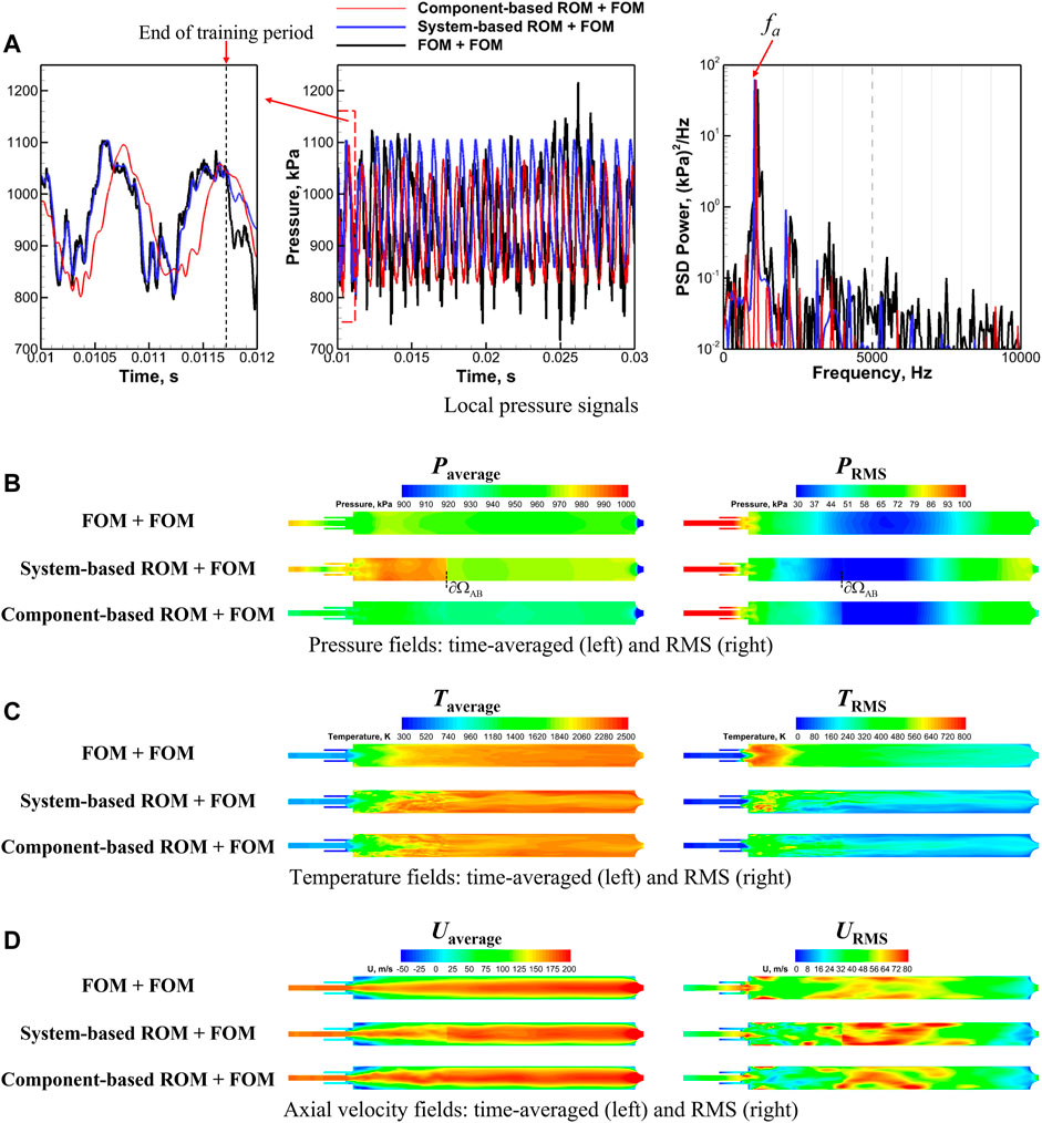
FIGURE 6. Comparisons of (A) pressure signals measured at x = 0 in (B) pressure, (C) temperature, and (D) axial velocity time-averaged (left) and root-mean-square (right) fields with different models (component-based ROM vs. system-based ROM vs. FOM) used for the upstream injector element (ΩA) for the single-injector combustor.
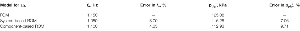
TABLE 1. Comparisons of the dominant acoustic frequency (fa) and the peak-to-peak pressure amplitudes
Second, we assess the predictive capabilities of the ROM-FOM framework based on two other QoIs, time-averaged and root-mean-square (RMS) fields of the state variables, which serve as crucial determining factors in many engineering applications
where nt is the total number of snapshots included to calculate the QoI, and Φn represents the state variable of interest, e.g., pressure (P), temperature (T), and axial (or streamwise) velocity (U), at time step n. In addition, the errors of the ROM-FOM framework in predicting Φaverage and ΦRMS are further quantified as follows
where Φ represents the QoIs (i.e., either the time-averaged or RMS field) for the error measurement, and Φref represents the QoIs calculated from the FOM-FOM framework. The errors, calculated based on Eq. 22, are summarized in Table 2. Though the ROM-FOM framework is able to provide reasonably accurate predictions of the time-averaged fields (
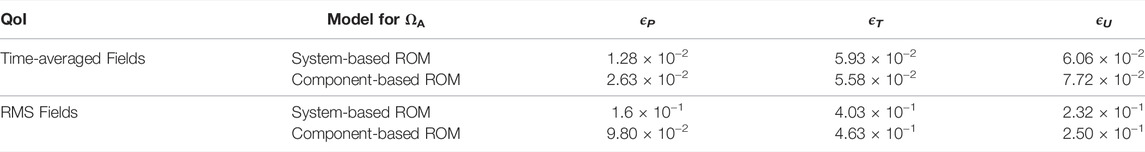
TABLE 2. Comparisons of the errors in predicting time-averaged and RMS fields of pressure (P), temperature(T), and axial velocity (U) corresponding to Figures 6B-D with different models (component-based ROM vs. system-based ROM) used for the upstream injector element for the single-injector combustor.
Such challenges and the limitation of using a linear and static basis set are further revealed by comparing the time-averaged and RMS fields between the FOM-FOM and ROM-FOM framework in Figures 6B–D, which shows significanly under-predicted magnitudes of the RMS fields by the ROM-FOM framework. More importantly, distinguishable mismatches between solutions in ΩA and ΩB are observed at the component interface ∂ΩAB in ROM-FOM results, featuring abrupt changes in numerical values in the regions adjacent to the interface (e.g., Paverage, Uaverage, URMS of system-based ROM-FOM and PRMS of component-based ROM-FOM), which is absent in FOM-FOM results. The mismatches can be mainly attributed to the inconsistent orders of modeling accuracy between ROM in ΩA, restricted by the POD basis, and FOM in ΩB, restricted by the mesh resolution. The use of a static linear basis for ROM in ΩA limits its predictive capabilities. It is pointed out that the interface mismatches are not unique to ROM/FOM coupling, but more general issues for finite-element [73] and finite-volume [74] methods, especially with non-matching grids (i.e., inconsistent orders of modeling accuracy)—for example, the coupling of low- and high-order CFD solvers (FOMs) may require—for example—an overset-mesh approach [21,75]. Though such methods can be effective in coupling of low- and high-order FOMs, it is not clear whether such methods can be applied directly to ROM and FOM coupling since ROM evolves on a reduced dimensional trajectory determined by the basis, while the FOM (either with low- or high-order numerical methods) solves the dynamical system on the full state space trajectory.
6.1.3 Performance Enhancement via Adaptive-Basis Reduced-Order Models
To address the above challenges, we seek to improve the ROM modeling accuracy via the one-step adaptive-basis approach introduced in Section 4. During the offline stage, 10 snapshots from the component-based ROM training demonstrated in Figure 5B are used to generate the initial POD basis
Following similar evaluation procedures as in Section 6.1.2, local pressure signals measured at x = 0 are first compared with the FOM-FOM results in Figures 7A–C for different combustor lengths. The peak-to-peak pressure oscillation amplitude
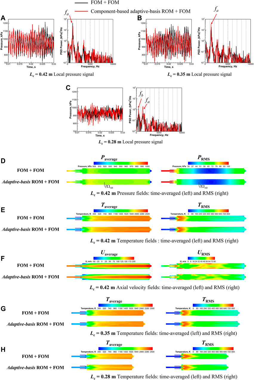
FIGURE 7. Comparisons of (A–C) pressure signals measured at x = 0 in Figure 4, time-averaged (left) and root-mean-square (right) (D) pressure, (E) temperature, and (F) axial velocity fields for Lc = 0.42 m, and time-averaged (left) and root-mean-square (right) temperature fields for Lc = (G) 0.35 and (H) 0.28 m with component-based adaptive-basis ROM and FOM used for the upstream injector element (ΩA) for the single-injector combustor.
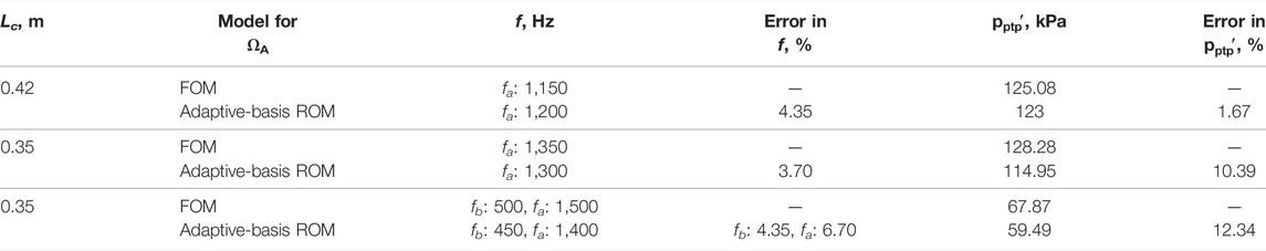
TABLE 3. Comparisons of the dominant acoustic frequency (f) and the peak-to-peak pressure amplitudes
Next, we extend the evaluations of adaptive-basis framework to the predictions of time-averaged and RMS fields defined in Eq. 21, the errors of which are calculated using Eq. 22 and summarized in Table 4. Significant improvement (e.g., approximately O(10) error reduction) in predicting the time-averaged and RMS fields of P, U, and T can be readily seen comparing Table 4 (rows corresponding to Lc = 0.42 m) and Table 2. The time-averaged and RMS fields predicted using adaptive-basis framework are investigated further in Figures 7D–F, which shows excellent agreement with the FOM-FOM results with the magnitudes of the RMS fields predicted correctly and no distinguishable interface mismatches observed in Figures 6B–D.
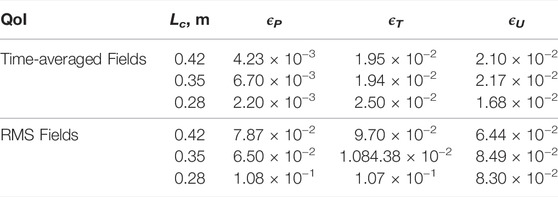
TABLE 4. Comparisons of the errors in predicting time-averaged and RMS fields of pressure (P), temperature(T), and axial velocity (U) using the framework corresponding to Figures 7D-H with adaptive-basis ROMs for the single-injector combustor with different combustor lengths (Lc).
Moreover, the adaptive-basis framework is demonstrated to be capable of predicting the time-averaged and RMS fields for different combustor lengths reasonably accurately as reflected in Table 4. Specifically, the time-averaged and RMS fields of temperature (T) are selected to further demonstrate the modeling capabilities of the adaptive-basis framework as shown in Figures 7G,H because the temperature dynamics is characterized by chaotic non-stationary and advection-dominated features as shown in Figure 4, which prove to be most challenging to represent with static-basis framework as shown in Figure 6. Overall, the adaptive-basis framework is able to represent the changes in the time-averaged and RMS temperature fields with variations in the combustor lengths.
6.2 Multi-Injector Model Rocket Combustor
Next, we proceed to demonstrate the component-based domain-decomposition framework on the multi-injector model rocket combustor configuration shown in Figure 8A, based on a laboratory rocket model engine [60], originally designed to study combustion instability of transverse acoustics. In Figure 8A, we take the five-injector configuration as an example for illustration and also consider the configurations with three and seven injectors to demonstrate the capabilities of the framework in the following sections. As seen in Figure 8A, this configuration consists of five shear coaxial injectors, each of which is similar to the single-injector geometry in Figure 4, and is featured with an outer passage, T1, that introduces fuel near the downstream end of the coaxial inner passage, T2, that feeds oxidizer to the combustion chamber. The operating conditions in all the multi-injector combustor configurations are maintained with an adiabatic flame temperature of approximately 2,700 K and a mean chamber pressure of 1.3 MPa. The T1 stream contains gaseous methane (100% CH4) at 300 K. The T2 stream is 42% gaseous O2 by mass and 58% gaseous H2O by mass at 660 K. Both the T1 and T2 streams are fed with constant mass flow rates, 0.67 kg/s and 19.75 kg/s, respectively. A non-reflective boundary condition is imposed at the downstream end of the computational domain with the goal of suppressing longitudinal acoustics in the streamwise direction, which promotes the generation of transverse acoustic waves in the spanwise direction. Similar to the single-injector configuration in Section 6.1, combustion is represented by the flamelet progress variable (FPV) model with GRI-1.2 chemical kinetics.
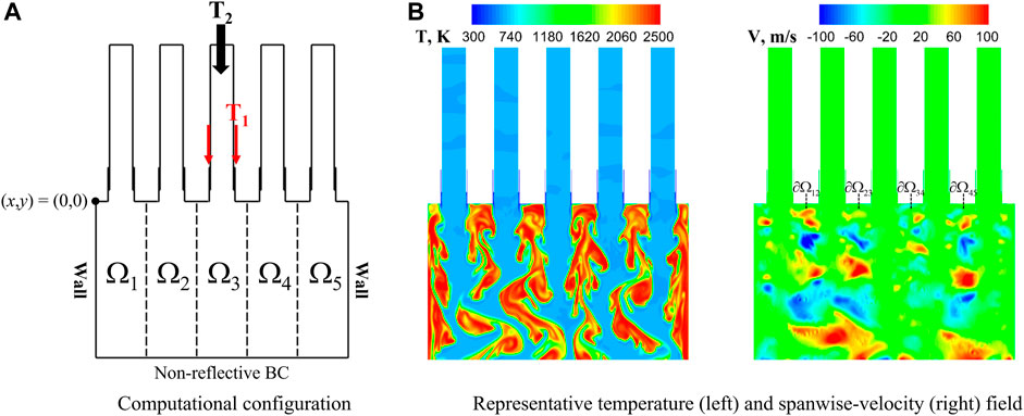
FIGURE 8. (A) Computational configuration and (B) representative temperature and spanwise-velocity field of 2D-planar multi-injector model rocket combustor.
As shown in Figure 8A, the five-injector model rocket combustor can be represented by two reference components, the interior injector element (e.g., Ω3) and the wall injector element (e.g., Ω5). Therefore, the multi-injector configuration can be modeled using two ROMs trained based on the reference components, denoted as an all-ROM framework, as illustrated in Section 5. With the ROM/FOM coupled framework demonstrated using the single-injector configuration, we use the multi-injector configuration to evaluate and demonstrate the ROM/ROM coupled framework.
When the FOM is adopted to model all five components, denoted as all-FOM framework, the resulting representative snapshots of the flow fields are shown in Figure 8B, which exhibits two major features that have not been observed in the single-injector case in Section 6.1: 1) stronger interactions between components, featured with large-scale vortex shedding approaching the downstream end of the domain; and 2) more complex dynamics at the component interfaces (i.e., ∂Ω12, ∂Ω23, ∂Ω34, and ∂Ω45), featured with both positive and negative spanwise velocity.
6.2.1 Injector-Element Reduced-Order Models Training and Framework Integration
In this section, we discuss the ROM training strategies based on the two different components (the interior and wall injector elements) identified above and how to integrate the two trained ROMs into the framework to model the multi-injector model rocket combustor. We focus on the component-based methods for ROM training as illustrated in Figures 9A,B corresponding to the interior and wall injector element respectively. To incorporate the strong interactions between injector elements observed in Figure 8B, two adjacent injector elements are included for interior injector-element ROM training (Figure 9A) while one additional adjacent injector element is added for wall injector-element ROM training (Figure 9B), which cannot be easily accounted by imposing boundary conditions directly as conceptualized in Figure 2 considering the complexity of the dynamics at the component interfaces. In addition, similar to the single-injector configuration, auxiliary domains with exponentially stretched mesh elements in the spanwise direction are added next to the additional injector elements in ROM training (two for interior injector-element and one for wall injector-element). This incorporates the complex dynamics at the component interfaces, especially for the abrupt changes in the directions of the flow characteristics (e.g., existence of both positive and negative spanwise velocity) observed in Figure 8B. Non-reflective boundary conditions are imposed at the downstream end for both the interior and wall injector element ROM training to be consistent with the target multi-injector configuration (Figure 8A). Forcing is imposed via non-reflective boundary conditions at the side boundaries with backward characteristics qu−c perturbed using the same function in Eq. 19 to generate the essential dynamics anticipated in the full system. Here, we choose to impose the forcing with A = 0 to mimic a broad-and response, which presumably contains rich responses in the frequency domain. The solution snapshots are extracted corresponding to the regions bounded by dashed lines in Figures 8A,B, which are then used to construct the interior injector-element ROM and the wall injector-element ROM, respectively. The resulting ROMs are coupled through the direct flux matching method at the component interfaces adopted to model all the interior injector elements (Ω2, Ω3, and Ω4 in Figure 8A) and
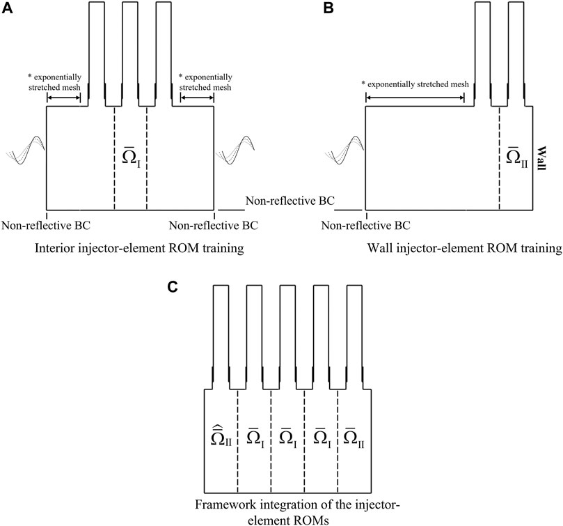
FIGURE 9. Component-based ROM training strategies for (A) the interior injector element and (B) the wall injector element and (C) the integration of the injector-element ROMs for the 2D-planar multi-injector model rocket combustor.
Since the two wall injector elements are geometrically identical (i.e., reflective symmetry) to each other,
6.2.2 Performance
Based on the investigations using the single-injector configuration in Section 6.1, we apply the adaptive-basis method, introduced in Section 4, to develop the two component-based ROMs,
Next, we proceed to evaluate the performance of the all-adaptive-basis-ROM framework based on the results from the FOM, which is taken as the ground truth solution. Figures 10A–C compares the local PSD predicted using the FOM and with the all-adaptive-basis-ROM framework, which are measured at the corner of the left wall, i.e., (x, y) = (0, 0) in Figure 8A for all 3 multi-injector configurations. Different from the single-injector cases in Section 6.1, the true pressure signals from the all-FOM results in the multi-injector configurations do not exhibit distinguishable coherent oscillating patterns as in Figure 4. This aspect can be expected to be more challenging to be predicted by the ROM.
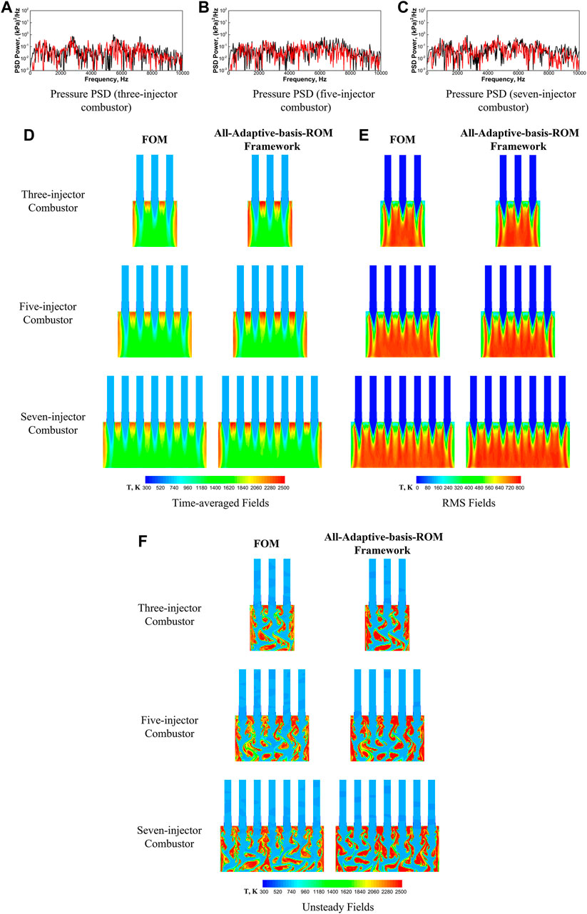
FIGURE 10. Comparisons of pressure PSDs (A–C) measured at (x, y) = (0, 0) in Figure 8 with different models (all-adaptive-basis-ROM (Red) framework vs. FOM (Black), (D) time-averaged, (E) RMS, and (F) unsteady temperature fields with different models (all-adaptive-basis-ROM framework vs. FOM) used in the framework for the three-injector (top), five-injector (middle), and seven-injector (bottom) configurations for the 2D-planar multi-injector model rocket combustor.
The predictions using the all-adaptive-basis-ROM framework show good agreement with the all-FOM framework results, especially in capturing the changes in PSD distributions due to the configuration variations with the number of injector elements increased from three to seven. For example, the wide-band frequency peak between 2,500 and 3,000 Hz in the three-injector combustor and the peak near 2,500 Hz for the seven-injector configuration are both well predicted by the all-adaptive-basis-ROM framework. More importantly, the broad-band PSD distributions (i.e., no identifiable frequency peaks) in the five-injector configuration are also accurately captured.
Having successfully demonstrated the ability of the adaptive ROM to capture changes in pressure oscillations arising from configuration variations, we next look at their ability to predict time-averaged and RMS fields of target state variables (P, U, and T) is assessed. The accuracy of the framework is evaluated based on the errors defined in Eq. 22, summarized in Table 5. It can be readily seen that the all-adaptive-basis-ROM framework is able to accurately predict the time-averaged fields of selected state variables with errors below 4% while even for the generally more challenging RMS fields, the prediction errors are shown to be below 18%, given the complexity and chaotic features of the dynamics present in the multi-injector problems, indicated by the broad-band frequency distributions in Figures 10A–C. Specifically, the time-averaged, RMS, and representative unsteady fields of temperature (T) are selected to demonstrate the predictive capabilities of the all-adaptive-basis-ROM framework as shown in Figures 10D,E for the three different multi-injector configurations, which exhibits good agreement between all-adaptive-basis-ROM and all-FOM framework results. But it still need to be pointed out that the all-adaptive-basis-ROM framework predicts elongated high-temperature zones between injector elements compared to the all-FOM framework results, indicating that the current methodology may require further improvement.
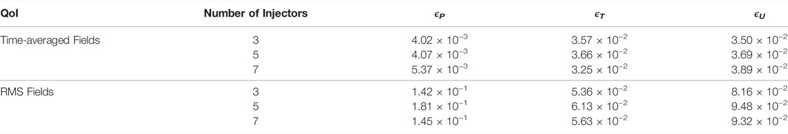
TABLE 5. Comparisons of the errors in predicting time-averaged and RMS fields of pressure (P), temperature(T), and axial velocity (U) corresponding to Figures 10D-E using the all-adaptive-basis-ROM framework for the multi-injector combustor.
7 Conclusion
A component-based domain-decomposition framework is established for the modeling of large-scale systems that cannot be directly accessed using the high-fidelity simulations (e.g., a rocket engine, a wind farm, and a compressor). This approach decomposes the full system into different components, each of which can flexibly adopt different modeling strategies (e.g., ROM or FOM), balancing physical complexity with accuracy requirements. Under the premise that most of the components share identical features and can be represented by a few reference components, a component-based reduced-order model (ROM) training strategy is proposed and demonstrated, which requires only the high-fidelity simulations of the individual components. System-level feedback and responses in the training dataset is emulated by imposing boundary forcing. This leads to a significant saving in computational cost during ROM training. The model-form preserving least-squares with variable transformation (MP-LSVT) ROM formulation is pursued with enhancement through basis adaptation to construct the component-based ROMs. The trained ROMs can be adopted to model components with identical geometric features and coupled with either a reduced-fidelity full-order model (RF-FOM) or ROMs via a direct flux matching method to enable both accurate and efficient simulations of large-scale systems with different geometric configurations.
Detailed evaluations of the framework were first performed based on a planar single-injector model rocket configuration with varying combustor lengths, each of which exhibit different dynamic behaviors. The framework separates the single-injector configuration into two components, the upstream injector element and the downstream combustor + nozzle, the former of which adopts MP-LSVT ROM for modeling, while the latter adopts a FOM. Two methods, (system-based and component-based) are used to train the injector-element ROM. It was demonstrated that the upstream-component ROMs from both training methods, when coupled with the downstream-component FOM, can produce reasonably accurate predictions of the pressure oscillations while the component-based method requires much less computational cost. However, the ROM/FOM framework encounters difficulties in representing the time-averaged and root-mean-square (RMS) fields of the target state variables while distinguishable solution mismatches are observed at the component interface. To address this limitation, basis adaptation is incorporated in the MP-LSVT formulation to enhance ROM capabilities, which significantly improves the predictive accuracy of the framework and more importantly, is capable of representing changes in dynamic behaviors due to the variations in combustor length.
The framework was then extended to a 2D-planar multi-injector model rocket configuration with different number of injector elements, which can be represented by two reference injector-element components. High-fidelity training simulations are then conducted on the two reference components to develop the component-based ROMs via MP-LSVT formulation with basis adaptation. The framework is demonstrated to be capable of predicting all the quantities-of-interest (QoIs) accurately, including local pressure oscillations, time-averaged and RMS fields of target state variables for the multi-injector configuration with different number of injector elements.
Though preliminary and demonstrated for only 2D problems, the component-based domain-decomposition framework with adaptive-basis ROMs is directly applicable to 3D problems and mostly importantly serves as a stepping stone towards modeling practical large-scale engineering systems (e.g., a RD-170 rocket engine [16]). Before this framework can be adopted by engineers in many-query applications (such as design and uncertainty quantification) of the full system, two major aspects need to be considered: 1) efficiency—hyper-reduction has to be considered to enable more efficient ROM calculations as mentioned in Section 4; and 2), scalability—the ROMs must be amenable for execution on memory-restricted computers such as desktop workstations or embedded systems—i.e., they need to be load-balanced and scalable in terms of computational resources available.
Discussions are provided by the current authors [14] on constructing scalable, load-balanced, and hyper-reduced static-basis ROMs while all these aspects remain to be further investigated for adaptive-basis ROM development. To address the remaining gaps, good avenue for future work can be on incorporating adaptive sparse sampling methods (e.g., [50]) in the adaptive-basis ROM to achieve computational efficiency enhancement, while exploring dynamic methods to achieve scalability when the sampling elements are getting adapted. In addition, the component-based framework is designed to be generally compatible with different types of ROM methods and hence instead of the intrusive ROM used in the current work, non-intrusive ROM methods [44,78] may also be considered for the future work.
Data Availability Statement
The raw data supporting the conclusion of this article will be made available by the authors upon request.
Author Contributions
CH, KD, and CM all contributed to formulation of the component-based reduced-order modeling framework and the component-based ROM training strategies. CH established the test problems, perform the numerical investigations, and wrote the first draft of the manuscript. KD formulated the adaptive-basis method provided in the manuscript and contributed to the method for ROM integration in the framework. CM formulated the component-based ROM framework and conceptualized its application for rocket combustion problems. All authors contributed to manuscript revision, read, and approved the submitted version.
Funding
The authors acknowledge support from the US Air Force under the Center of Excellence grant FA9550-17-1-0195, titled Multi-Fidelity Modeling of Rocket Combustor Dynamics (Program Managers: Dr. Mitat Birkan, Dr. Fariba Fahroo, and Dr. Ramakanth Munipalli).
Conflict of Interest
The authors declare that the research was conducted in the absence of any commercial or financial relationships that could be construed as a potential conflict of interest.
Publisher’s Note
All claims expressed in this article are solely those of the authors and do not necessarily represent those of their affiliated organizations, or those of the publisher, the editors and the reviewers. Any product that may be evaluated in this article, or claim that may be made by its manufacturer, is not guaranteed or endorsed by the publisher.
References
1. Wang ZJ, Li Y, Jia F, Laskowski GM, Kopriva J, Paliath U, et al. Towards Industrial Large Eddy Simulation Using the Fr/cpr Method. Comput Fluids (2017) 156:579–89. doi:10.1016/j.compfluid.2017.04.026
2. Aditya K, Gruber A, Xu C, Lu T, Krisman A, Bothien MR, et al. Direct Numerical Simulation of Flame Stabilization Assisted by Autoignition in a Reheat Gas Turbine Combustor. Proc Combustion Inst (2019) 37:2635–42. doi:10.1016/j.proci.2018.06.084
3. Oefelein JC. Advances in Modeling Supercritical Fluid Behavior and Combustion in High-Pressure Propulsion Systems. AIAA Scitech Forum (2019):0634. doi:10.2514/6.2019-0634
4. Lumley JL, Poje A. Low-dimensional Models for Flows with Density Fluctuations. Phys Fluids (1997) 9:2023–31. doi:10.1063/1.869321
5. Graham W, Peraire J, Tang K. Optimal Control of Vortex Shedding Using Low Order Models Part I: Open-Loop Model Development. Int J Numer Methods (1997) 44:945–72. doi:10.1002/(SICI)1097-0207(19990310)44:7<973::AID-NME538>3.0
6. Lucia DJ, Beran PS. Projection Methods for Reduced Order Models of Compressible Flows. J Comput Phys (2003) 188:252–80. doi:10.1016/s0021-9991(03)00166-9
7. Barbagallo A, Sipp D, Schmid PJ. Closed-loop Control of an Open Cavity Flow Using Reduced-Order Models. J Fluid Mech (2009) 641:1–50. doi:10.1017/s0022112009991418
8. Barbagallo A, Sipp D, Schmid PJ. Input–output Measures for Model Reduction and Closed-Loop Control: Application to Global Modes. J Fluid Mech (2011) 685:23–53. doi:10.1017/jfm.2011.271
9. Barbagallo A, Dergham G, Sipp D, Schmid PJ, Robinet JC. Closed-loop Control of Unsteadiness over a Rounded Backward-Facing Step. J Fluid Mech (2012) 703:326–62. doi:10.1017/jfm.2012.223
10. Lucia DJ, Beran PS, Silva WA. Reduced-order Modeling: New Approaches for Computational Physics. Prog Aerospace Sci (2004) 40:51–117. doi:10.1016/j.paerosci.2003.12.001
11. Lieu T, Farhat C. Adaptation of Aeroelastic Reduced-Order Models and Application to an F-16 Configuration. AIAA J (2007) 45:1244–57. doi:10.2514/1.24512
12. Blonigan PJ, Carlberg K, Rizzi F, Howard M, Fike JA. Model Reduction for Hypersonic Aerodynamics via Conservative LSPG Projection and Hyper-Reduction. AIAA J. (2021) 59 (4):1296–1312.
13. Huang C, Duraisamy K, Merkle CL. Investigations and Improvement of Robustness of Reduced-Order Models of Reacting Flow. AIAA J (2019) 57:5377–89. doi:10.2514/1.j058392
14. Huang C, Wentland CR, Duraisamy K, Merkle C. Model Reduction for Multi-Scale Transport Problems Using Model-form Preserving Least-Squares Projections with Variable Transformation. J Comput Phys (2022) 448:110742. doi:10.1016/j.jcp.2021.110742
15. Urbano A, Selle L, Staffelbach G, Cuenot B, Schmitt T, Ducruix S, et al. Exploration of Combustion Instability Triggering Using Large Eddy Simulation of a Multiple Injector Liquid Rocket Engine. Combustion and Flame (2016) 169:129–40. doi:10.1016/j.combustflame.2016.03.020
16. Fedorov V, Chvanov V, Chelkis F, Ivanov N, Lozinskay I, Buryak A. The Chamber Cooling System of Rd-170 Engine Family: Design, Parameters, and Hardware Investigation Data. Sacramento, CA, USA: AIAA/ASME/SAE/ASEE Joint Propulsion Conference & Exhibit (2006). doi:10.2514/6.2006-4363
17. Maday Y, Ronquist EM. A Reduced-Basis Element Method. J Scientific Comput (2002) 17:447–59. doi:10.1023/a:1015197908587
18. Iapichino L, Quarteroni A, Rozza G. Reduced Basis Method and Domain Decomposition for Elliptic Problems in Networks and Complex Parametrized Geometries. Comput Math Appl (2016) 71:408–30. doi:10.1016/j.camwa.2015.12.001
19. Phuong Huynh DB, Knezevic DJ, Patera AT. A Static Condensation Reduced Basis Element Method : Approximation Anda Posteriorierror Estimation. ESAIM: Math Model Numer Anal (2012) 47:213–51. doi:10.1051/m2an/2012022
20. Gropp WD, Keyes DE. Domain Decomposition Methods in Computational Fluid Dynamics. Int J Numer Methods Fluids (1992) 14:147–65. doi:10.1002/fld.1650140203
21. Sitaraman J, Floros M, Wissink A, Potsdam M. Parallel Domain Connectivity Algorithm for Unsteady Flow Computations Using Overlapping and Adaptive Grids. J Comput Phys (2010) 229:4703–23. doi:10.1016/j.jcp.2010.03.008
22. Chaturantabut S, Beattie C, Gugercin S. Structure-preserving Model Reduction for Nonlinear Port-Hamiltonian Systems. SIAM J Sci Comput (2016) 38:B837–65. doi:10.1137/15m1055085
23. Gugercin S, Polyuga RV, Beattie C, van der Schaft A. Structure-preserving Tangential Interpolation for Model Reduction of Port-Hamiltonian Systems. Automatica (2012) 48:1963–74. doi:10.1016/j.automatica.2012.05.052
24. Califano F, Rashad R, Schuller FP, Stramigioli S. Energetic Decomposition of Distributed Systems with Moving Material Domains: The Port-Hamiltonian Model of Fluid-Structure Interaction. J Geometry Phys (2022) 175:104477. doi:10.1016/j.geomphys.2022.104477
25. Willcox K, Peraire J, Paduano JD. Application of Model Order Reduction to Compressor Aeroelastic Models. J Eng Gas Turbine Power (2002) 124:332–9. doi:10.1115/1.1416152
26. Maday Y, Ronquist EM. The Reduced Basis Element Method: Application to a thermal Fin Problem. SIAM J Sci Comput (2004) 26:240–58. doi:10.1137/s1064827502419932
27. Iapichino L, Quarteroni A, Rozza G. A Reduced Basis Hybrid Method for the Coupling of Parametrized Domains Represented by Fluidic Networks. Comput Methods Appl Mech Eng (2012) 221-222:63–82. doi:10.1016/j.cma.2012.02.005
28. Eftang JL, Patera AT. A Port-Reduced Static Condensation Reduced Basis Element Method for Large Component-Synthesized Structures: Approximation and A Posteriori Error Estimation.” in Advanced Modeling and Simulation in Engineering Sciences (2013).
29. Smetana K, Patera AT. Optimal Local Approximation Spaces for Component-Based Static Condensation Procedures. SIAM J Sci Comput (2016) 38:A3318–56. doi:10.1137/15m1009603
30. Kapteyn MG, Knezevic DJ, Huynh DBP, Tran M, Willcox KE. Data-driven Physics-Based Digital Twins via a Library of Component-Based Reduced-Order Models. Int J Numer Methods Eng (2020) 123:2986–3003. doi:10.1002/nme.6423
31. McBane S, Choi Y. Component-wise Reduced Order Model Lattice-type Structure Design. Comput Methods Appl Mech Eng (2021) 381:113813. doi:10.1016/j.cma.2021.113813
32. Lucia DJ, King PI, Beran PS. Reduced Order Modeling of a Two-Dimensional Flow with Moving Shocks. Computers & Fluids (2003) 32(7):917-38.
33. Buffoni M, Telib H, Iollo A. Iterative Methods for Model Reduction by Domain Decomposition. Comput Fluids (2009) 38:1160–7. doi:10.1016/j.compfluid.2008.11.008
34. Baiges J, Codina R, Idelsohn S. A Domain Decomposition Strategy for Reduced Order Models. Application to the Incompressible Navier–Stokes Equations. Comput Methods Appl Mech Eng (2013) 267:23–42. doi:10.1016/j.cma.2013.08.001
35. Ahmed SE, San O, Kara K, Younis R, Rasheed A. Multifidelity Computing for Coupling Full and Reduced Order Models. PLoS One (2021) 16:e0246092. doi:10.1371/journal.pone.0246092
36. Hoang C, Choi Y, Carlberg K. Domain-decomposition Least-Squares Petrov–Galerkin (Dd-lspg) Nonlinear Model Reduction. Comput Methods Appl Mech Eng (2021) 384:113997. doi:10.1016/j.cma.2021.113997
37. Xiao D, Fang F, Heaney CE, Navon IM, Pain CC. A Domain Decomposition Method for the Non-intrusive Reduced Order Modelling of Fluid Flow. Comput Methods Appl Mech Eng (2019) 354:307–30. doi:10.1016/j.cma.2019.05.039
38. Xiao D, Heaney CE, Fang F, Mottet L, Hu R, Bistrian DA, et al. A Domain Decomposition Non-intrusive Reduced Order Model for Turbulent Flows. Comput Fluids (2019) 182:15–27. doi:10.1016/j.compfluid.2019.02.012
39. Xiao C, Leeuwenburgh O, Lin HX, Heemink A. Efficient Estimation of Space Varying Parameters in Numerical Models Using Non-intrusive Subdomain Reduced Order Modeling. J Comput Phys (2021) 424:109867. doi:10.1016/j.jcp.2020.109867
40. Huang C, Anderson WE, Merkle CL, Sankaran V. Multifidelity Framework for Modeling Combustion Dynamics. AIAA J (2019) 57:2055–68. doi:10.2514/1.J057061
41. Xu J, Huang C, Duraisamy K. Reduced-order Modeling Framework for Combustor Instabilities Using Truncated Domain Training. AIAA J (2020) 58:618–32. doi:10.2514/1.J057959
42. Butcher J. Numerical Methods for Ordinary Differential Equations. John Wiley & Sons (2016). p. 333–87. doi:10.1002/9781119121534.ch4
43. Carlberg K, Barone M, Antil H. Galerkin V. Least-Squares Petrov-Galerkin Projection in Nonlinear Model Reduction. J Comput Phys (2017) 330:693–734. doi:10.1016/j.jcp.2016.10.033
44. McQuarrie SA, Huang C, Willcox KE. Data-driven Reduced-Order Models via Regularised Operator Inference for a Single-Injector Combustion Process. J R Soc New Zealand (2021) 51:194–211. doi:10.1080/03036758.2020.1863237
45. Amsallem D, Zahr MJ, Washabaugh K. Fast Local Reduced Basis Updates for the Efficient Reduction of Nonlinear Systems with Hyper-Reduction. Adv Comput Math (2015) 41:1187–230. doi:10.1007/s10444-015-9409-0
46. Geelen R, Willcox K. Localized Non-intrusive Reduced-Order Modeling in the Operator Inference Framework. Phil. Trans. R. Soc. A. (2021):3802021020620210206. doi:10.1098/rsta.2021.0206
47. Lee K, Carlberg KT. Model Reduction of Dynamical Systems on Nonlinear Manifolds Using Deep Convolutional Autoencoders. J Comput Phys (2020) 404:108973. doi:10.1016/j.jcp.2019.108973
48. Kim Y, Choi Y, Widemann D, Zohdi T. A Fast and Accurate Physics-Informed Neural Network Reduced Order Model with Shallow Masked Autoencoder. J Comput Phys (2022) 451:110841. doi:10.1016/j.jcp.2021.110841
49. Peherstorfer B, Willcox K. Online Adaptive Model Reduction for Nonlinear Systems via Low-Rank Updates. SIAM J Sci Comput (2015) 37:A2123–50. doi:10.1137/140989169
50. Peherstorfer B. Model Reduction for Transport-Dominated Problems via Online Adaptive Bases and Adaptive Sampling. SIAM J Sci Comput (2020) 42:A2803–36. doi:10.1137/19M1257275
51. Zimmermann R, Peherstorfer B, Willcox K. Geometric Subspace Updates with Applications to Online Adaptive Nonlinear Model Reduction. SIAM J Matrix Anal Appl (2018) 39:234–61. doi:10.1137/17m1123286
52. Chaturantabut S, Sorensen DC. Nonlinear Model Reduction via Discrete Empirical Interpolation. SIAM J Sci Comput (2010) 32:2737–64. doi:10.1137/090766498
53. Everson R, Sirovich L. Karhunen–Loève Procedure for Gappy Data. J Opt Soc Am A (1995) 12:1657. doi:10.1364/JOSAA.12.001657
54. Shipley K. Multi-injector Modeling of Transverse Combustion Instability Experiments (2014).Thesis
55. Harvazinski ME, Gejji R, Talley DG, Orth MR, Anderson WE, Pourpoint TL, et al. "Modeling of Transverse Combustion Instability," in AIAA Scitech. San Diego, CA, USA (2019), 1732
56. Henning P, Peterseim D. Oversampling for the Multiscale Finite Element Method. Multiscale Model Simul (2013) 11:1149–75. doi:10.1137/120900332
57. Comer AL, Huang C, Sardeshmukh S, Rankin BA, Harvazinski ME, Sankaran V, et al. Sensitivity Analysis of bluff-body Stabilized Premixed Flame Large-Eddy Simulations. J Propulsion Power (2021) 37:211–22. doi:10.2514/1.B37801
58. Harvazinski ME, Huang C, Sankaran V, Feldman TW, Anderson WE, Merkle CL, et al. Coupling between Hydrodynamics, Acoustics, and Heat Release in a Selfexcited Unstable Combustor. Phys Fluids (2015) 27:045102. doi:10.1063/1.4916673
59. Yu Y, Sisco JC, Rosen S, Madhav A, Anderson WE. Spontaneous Longitudinal Combustion Instability in a Continuously-Variable Resonance Combustor. J Propulsion Power (2012) 28:876–87. doi:10.2514/1.b34308
60. Morgan CJ, Shipley KJ, Anderson WE. Comparative Evaluation between experiment and Simulation for a Transverse Instability. J Propulsion Power (2015) 31:1696–706. doi:10.2514/1.B35759
61. Huang C, Gejji R, Anderson W, Yoon C, Sankaran V. Combustion Dynamics in a Single-Element Lean Direct Injection Gas Turbine Combustor. Combustion Sci Technol (2019) 192:2371–98. doi:10.1080/00102202.2019.1646732
62. Roe P. Approximate Riemann Solvers, Parameter Vectors, and Difference Schemes. J Comput Phys (1981) 43:357–72. doi:10.1016/0021-9991(81)90128-5
63. Mitchell C. Improved Reconstruction Schemes for the Navier–Stokes Equations on Unstructured Meshes. Reno, NV, USA: 32nd Aerospace Sciences Meeting and Exhibit (1994). doi:10.2514/6.1994-642
64. Barth T, Jespersen D. The Design and Application of Upwind Schemes on Unstructured Meshes. Reno, NV, USA: 27th Aerospace Sciences Meeting (1989). doi:10.2514/6.1989-366
65. Pierce CD, Moin P. Progress-variable Approach for Large-Eddy Simulation of Non-premixed Turbulent Combustion. J Fluid Mech (2004) 504:73–97. doi:10.1017/s0022112004008213
66. Frenklach M, Wang H, Goldenberg M, Smith G, Golden D, Bowman C, et al. GRI-Mech—an Optimized Detailed Chemical Reaction Mechanism for Methane Combustion. Gas Research Institute topical report no. GRI-95/0058 (1995).
67. Coclite A, Pascazio G, De Palma P, Cutrone L, Ihme M. An SMLD Joint PDF Model for Turbulent Non-premixed Combustion Using the Flamelet Progress-Variable Approach. Flow Turbul Combust (2015) 95:97–119. doi:10.1007/s10494-015-9609-1
68. Lee K, Carlberg KT. Model Reduction of Dynamical Systems on Nonlinear Manifolds Using Deep Convolutional Autoencoders. J Comput Phys (2020) 404:108973. doi:10.1016/j.jcp.2019.108973
69. Barone M, Kalashnikova I, Segalman D, Heidi K. Stable Galerkin Reduced Order Models for Linearized Compressible Flow. J Comput Phys (2009) 228:1932–46. doi:10.1016/j.jcp.2008.11.015
70. San O, Maulik R. Neural Network Closures for Nonlinear Model Order Reduction. Adv Comput Math (2018) 44:1717–50. doi:10.1007/s10444-018-9590-z
71. Stabile G, Ballarin F, Zuccarino G, Rozza G. A Reduced Order Variational Multiscale Approach for Turbulent Flows. Adv Comput Math (2019) 45:2349–68. doi:10.1007/s10444-019-09712-x
72. Grimberg S, Farhat C, Youkilis N. On the Stability of Projection-Based Model Order Reduction for Convection-Dominated Laminar and Turbulent Flows. J Comput Phys (2020) 419:109681. doi:10.1016/j.jcp.2020.109681
73. Farhat C, Macedo A, Lesoinne M, Roux FX, Magoules F, Bourdonnaie AL, et al. Two-level Domain Decomposition Methods with lagrange Multipliers for the Fast Iterative Solution of Acoustic Scattering Problems. Comput Methods Appl Mech Eng (2000) 184:213–39. doi:10.1016/s0045-7825(99)00229-7
74. Saas L, Faille I, Nataf F, Willien F. Finite Volume Methods for Domain Decomposition on Nonmatching Grids with Arbitrary Interface Conditions. SIAM J Numer Anal (2005) 43:860–90. doi:10.1137/s0036142903434059
75. Brazell MJ, Sitaraman J, Mavriplis DJ. An Overset Mesh Approach for 3d Mixed Element High-Order Discretizations. J Comput Phys (2016) 322:33–51. doi:10.1016/j.jcp.2016.06.031
76. Drmač Z, Gugercin S. A New Selection Operator for the Discrete Empirical Interpolation Method—Improved A Priori Error Bound and Extensions. SIAM J Sci Comput (2016) 38:A631–48. doi:10.1137/15m1019271
77. Peherstorfer B, Drmač Z, Gugercin S. Stability of Discrete Empirical Interpolation and Gappy Proper Orthogonal Decomposition with Randomized and Deterministic Sampling Points. SIAM J Sci Comput (2020) 42:A2837–64. doi:10.1137/19M1307391
Keywords: reduced order modeling, domain decomposition, model reduction, turbulent reacting flows, adaptive basis
Citation: Huang C, Duraisamy K and Merkle C (2022) Component-Based Reduced Order Modeling of Large-Scale Complex Systems. Front. Phys. 10:900064. doi: 10.3389/fphy.2022.900064
Received: 19 March 2022; Accepted: 16 May 2022;
Published: 24 August 2022.
Edited by:
Traian Iliescu, Virginia Tech, United StatesReviewed by:
Tommaso Taddei, Institut National de Recherche en Informatique et en Automatique (INRIA), FranceLuca Dede', Politecnico di Milano, Italy
Copyright © 2022 Huang, Duraisamy and Merkle. This is an open-access article distributed under the terms of the Creative Commons Attribution License (CC BY). The use, distribution or reproduction in other forums is permitted, provided the original author(s) and the copyright owner(s) are credited and that the original publication in this journal is cited, in accordance with accepted academic practice. No use, distribution or reproduction is permitted which does not comply with these terms.
*Correspondence: Cheng Huang, Y2hlbmdodWFuZ0BrdS5lZHU=