Giant-Cavity-Based Quantum Sensors With Enhanced Performance

Recent progress has revealed that quantum systems with multiple position-dependent couplings, e.g., giant atoms, can exhibit some unconventional phenomena, such as non-exponential decay. However, their potential applications are still open questions. In this paper, we propose a giant-cavity-based quantum sensor for the first time, whose performance can be greatly enhanced compared to traditional cavity-based sensors. In our proposal, two cavities are coupled to a dissipative reservoir at multiple points while they couple to a gain reservoir in a single-point way. To detect an unknown parameter entering the sensor, a waveguide is coupled to one of the cavities where detecting fields can pass through for homodyne detection. We find that multiple position-dependent couplings can induce an inherent non-reciprocal coupling between the cavities, which can enhance the performance of sensors. Compared to the results in the work of Lau and Clerk, (Nat Commun, 2018, 9: 4,320), our output noise can remain at the shot noise level, which is about one order of magnitude lower. In addition, the signal-to-noise ratio per photon is also enhanced by about one order of magnitude. These results showed that the multiple-point coupling structure is beneficial to existing quantum devices.

1 Introduction

High-precision measurement of physical quantities lies in the core of metrology, e.g., gravitational wave detection [1, 2], nano-particle detection [3–6], thermal sensing [7], navigation [8, 9], and magnetometers [10–12]. Towards fundamental detection limits in weak-signal measurements, non-reciprocity [13] has become a powerful resource [14]. Since reciprocity is hard to break due to Lorentz theorem [15], many methods have been proposed for inducing non-reciprocity, for example, biasing with odd-symmetric quantities under time reversal [16], steering systems into exceptional points [17,18], constructing directional couplings [19], employing asymmetric or non-linear elements [20–29], or breaking the time-invariance of systems [30, 31].

Recent progress on quantum systems with multiple-point couplings (e.g., giant atoms [32–48]) provides a new possibility to acquire non-reciprocity. For example, when several giant atoms couple to a common reservoir, an indirect coupling among atoms can be built up via the shared reservoir. This indirect coupling depends on the arrangements of atoms and the relative phase between coupling points [36]. Therefore, one can construct an effective directional coupling between atoms by tuning the relative phase and adjusting the arrangements. It should be noticed that the non-reciprocity realized in this way is an inherent property of the system and it can be totally tuned by the relative phase, such that this method of acquiring non-reciprocity requires no other non-linear elements such as Faraday rotators [20, 21] or Josephson parametric converters [26, 28], and thus, it is easy to be integrated into an on-chip structure and flexible in experiments.

In this study, we propose a quantum sensor consisting of two giant cavities, where two coupled cavities couple to reservoirs at multiple points. We find that an inherent non-reciprocal coupling between cavities can be built up through a shared reservoir. Compared with the small-cavity-based structures in [14], i.e., cavities couple to reservoirs at a single point, the signal-to-noise ratio in our proposal can be improved by one order of magnitude. The study is organized as follows. In Section 2, we propose the theoretical model of the quantum sensor, including the Hamiltonian and equations of motion. Following the standard frame [14], we propose the performance indicator of sensors in Section 3, including signal, output noise, and signal-to-noise ratio per photon. The comparison with the sensor made up of small cavities is shown in Section 4. Finally, further discussion and conclusion are given in Section 5.

2 Model of Gaint-Cavity-Based Quantum Sensor

2.1 Hamiltonian

Generally speaking, a quantum sensor means the sensor utilizing quantum resources, such as quantum devices, quantum states, quantum effects, etc. [49, 50]. In [14], a paradigm in designing quantum sensors is proposed that several coupled cavities couple to a gain reservoir and a dissipative reservoir at a single point. Illuminated by this paradigm, the sensor we considered consists of a coupled double-cavity interacting with two reservoirs. The first cavity is coupled to a dissipative reservoir at x₁ and x₂, and the second cavity is coupled to it at x₃ and x₄, as shown in Figure 1. On the contrary, a gain reservoir couples to both cavities at the same point. In addition, a classical pump β with a noise input B_in enters the readout waveguide which only couples to the cavity 1, and its reflected field B_out is measured by homodyne detection. This model can be realized by superconducting quantum circuits, i.e., two LC resonators couple to three waveguides, where one of the waveguides is used for readout and the others are used as reservoirs. According to the model, the total Hamiltonian reads

$H_{\text{tot}}=H_0+H_d+H_I,(1)$

where

$H_0=\sum _{\mathrm{i},\mathrm{j}=\mathrm{1}}^2{H}_{\text{ij}}\left[\epsilon \right]a_{\mathrm{i}}^{†}{a}_{\mathrm{j}}+\int \mathrm{d}k{\omega }_{b,k}{b}_k^{†}{b}_k+\int \mathrm{d}k{\omega }_{c,k}{c}_k^{†}{c}_k+\int \mathrm{d}k{\omega }_{d,k}{d}_k^{†}{d}_k,(\mathrm{2a})$

$H_d=\sqrt{\kappa }\left(\beta e^{-i{\omega }_{L}t}{a}_1^{†}+H.c.\right)+\sqrt{\kappa }\int \frac{\mathrm{d}k}{\sqrt{2\pi }}\left(a_1^{†}{b}_k+H.c.\right),(\mathrm{2b})$

$H_I=\sum _{\mathrm{i}=1}^2\int \mathrm{d}k\left(Y_{\mathrm{i}}{a}_{\mathrm{i}}^{†}{c}_k^{†}+H.c.\right)+\int \mathrm{d}k\left(Z_1\left(e^{ik{x}_1}+e^{ik{x}_2}\right)a_1^{†}{d}_k+Z_2\left(e^{ik{x}_3}+e^{ik{x}_4}\right)a_2^{†}{d}_k+H.c.\right).(\mathrm{2c})$

FIGURE 1

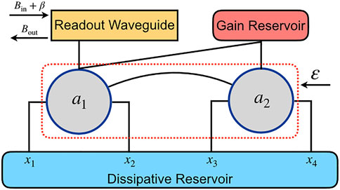
FIGURE 1. Schematic of the two giant-cavity quantum sensor. Both cavities couple to a dissipative reservoir at multiple points, i.e., x₁ and x₂ for cavity 1 (denoted by annihilation operator a₁), x₃ and x₄ for cavity 2 (denoted by operator a₂). The distance between the two points for one cavity is sufficiently large, which induces non-negligible time delays, such that it forms two giant cavities. As a result, the couplings between cavities and dissipative reservoir are position-dependent. On the contrary, both cavities couple to the gain reservoir at the same point. Also, a classical pump with an amplitude β and a noise input B_in is injected into the readout waveguide which only couples to the cavity 1. Its reflected field B_out is measured by homodyne detection. Initially, both reservoirs and the waveguide are prepared in the vacuum state. This sensor can reflect the external perturbation ɛ from the variations of the output B_out.

Equation 2a describes the free Hamiltonian of the two cavities, the readout waveguide, the gain and dissipative reservoirs with bosonic annihilation operators a_i, b_k, c_k, and d_k, respectively. Here, we have assumed that the perturbation ɛ is small enough such that H_ij [ɛ] has a linear form¹ [14, 51] $H_{\text{ij}}[\epsilon ]=H_{\text{ij}}^f+\epsilon V_{\text{ij}}$, where $H_{\text{ij}}^f$ is the unperturbed part of the coupled cavities and V_ij denotes the coupling of perturbation ɛ on the cavities. The first term in Eq. 2b represents a classical pump β with a driving frequency ω_L and a coupling strength κ that enters cavity 1 through the readout waveguide. The second term denotes the interaction between cavity 1 and the readout waveguide, which yields a noise input B_in to the cavity, as shown later. Eq. 2c describes couplings between the cavities and the reservoirs with strengths Y_i and Z_i, respectively. Notably, the position-dependent phase $e^{ik{x}_m},$ (m = 1, 2, 3, 4) with a wave vector k is introduced by the multi-point couplings.

2.2 Langevin Equations

For the sake of sensing, we analyze how the output varies when the perturbation ɛ acts on the sensor, which can be done with the quantum Langevin equation. Before we proceed, we assume that the coupling points are equally spaced, i.e., d = x₂ − x₁ = x₃ − x₂ = x₄ − x₃. For simplicity, we let x₁ = 0. Also, the linear dispersion relation holds in the dissipative reservoir, i.e., ω_d,k = v_gk with v_g being the group velocity [48, 52, 53]. With the abovementioned assumptions, the equations of motion for two cavities take the form

${\dot{\stackrel{̃}{a}}}_1\left[t\right]=F_{11}\left[\epsilon \right]{\tilde{a}}_1\left[t\right]-2\pi |Z_1{|}^2{\tilde{a}}_1\left[t-\tau \right]e^{i{\omega }_L\tau }+F_{12}\left[\epsilon \right]{\tilde{a}}_2\left[t\right]-{\tilde{M}}_1^{\text{in}}\left[t\right],(\mathrm{3a})$

${\dot{\stackrel{̃}{a}}}_2\left[t\right]=F_{22}\left[\epsilon \right]{\tilde{a}}_2\left[t\right]-2\pi |Z_2{|}^2{\tilde{a}}_2\left[t-\tau \right]e^{i{\omega }_L\tau }+F_{21}\left[\epsilon \right]{\tilde{a}}_1\left[t\right]-F_{21}^{\text{dir}}\left[t\right]-{\tilde{M}}_2^{\text{in}}\left[t\right],(\mathrm{3b})$

where

$F_{11}\left[\epsilon \right]=i{\omega }_L-i{H}_{11}\left[\epsilon \right]+\pi |Y_1{|}^2-2\pi |Z_1{|}^2-\frac{\kappa }{2},(\mathrm{4a})$

$F_{22}\left[\epsilon \right]=i{\omega }_L-i{H}_{22}\left[\epsilon \right]+\pi |Y_2{|}^2-2\pi |Z_2{|}^2,(\mathrm{4b})$

$F_{12}\left[\epsilon \right]=-i{H}_{12}\left[\epsilon \right]+\pi Y_1{Y}_2^{\ast },(\mathrm{4c})$

$F_{21}\left[\epsilon \right]=-i{H}_{21}\left[\epsilon \right]+\pi Y_2{Y}_1^{\ast },(\mathrm{4d})$

$F_{21}^{\text{dir}}\left[t\right]=2\pi Z_2{Z}_1^{\ast }{e}^{i{\omega }_L\tau }\left({\tilde{a}}_1\left[t-\tau \right]+2{\tilde{a}}_1\left[t-2\tau \right]e^{i{\omega }_L\tau }+{\tilde{a}}_1\left[t-3\tau \right]e^{2i{\omega }_L\tau }\right),(4e)$

${\tilde{M}}_1^{\text{in}}\left[t\right]=i\sqrt{\kappa }\left(\beta +{\tilde{B}}_{\text{in}}\left[t\right]\right)-i\sqrt{2\pi }{Y}_1{\tilde{C}}_{\text{in}}^{†}\left[t\right]-i\sqrt{2\pi }{Z}_1\left({\tilde{D}}_{\text{in}}\left[t\right]+{\tilde{D}}_{\text{in}}\left[t-\tau \right]e^{i{\omega }_L\tau }\right),(\mathrm{4f})$

${\tilde{M}}_2^{\text{in}}\left[t\right]=i\sqrt{2\pi }{Y}_2{\tilde{C}}_{\text{in}}^{†}\left[t\right]-i\sqrt{2\pi }{Z}_2{e}^{2i{\omega }_L\tau }\left({\tilde{D}}_{\text{in}}\left[t-2\tau \right]+{\tilde{D}}_{\text{in}}\left[t-3\tau \right]e^{i{\omega }_L\tau }\right),(\mathrm{4g})$

with τ = d/v_g being the time delay between the two neighboring points. Here, ${\tilde{a}}_{\mathrm{i}}[t]=a_{\mathrm{i}}[t]e^{i{\omega }_{L}t}$ denotes the slowly-varying operator. Also,

${\tilde{B}}_{\text{in}}\left[t\right]=B_{\text{in}}\left[t\right]e^{i{\omega }_{L}t}=\frac{1}{\sqrt{2\pi }}\int \mathrm{d}k{b}_k\left[0\right]e^{-i\left({\omega }_{b,k}-{\omega }_L\right)t},(\mathrm{5a})$

${\tilde{C}}_{\text{in}}^{†}\left[t\right]=C_{\text{in}}^{†}\left[t\right]e^{i{\omega }_{L}t}=\frac{1}{\sqrt{2\pi }}\int \mathrm{d}k{c}_k^{†}\left[0\right]e^{i\left({\omega }_{c,k}+{\omega }_L\right)t},(\mathrm{5b})$

${\tilde{D}}_{\text{in}}\left[t\right]=D_{\text{in}}\left[t\right]e^{i{\omega }_{L}t}=\frac{1}{\sqrt{2\pi }}\int \mathrm{d}k{d}_k\left[0\right]e^{-i\left({\omega }_{d,k}-{\omega }_L\right)t}(\mathrm{5c})$

are the inputs for the readout waveguide, gain, and dissipative reservoirs, respectively. In addition, the input-output relation for the field in the readout waveguide is given by

${\tilde{B}}_{\text{out}}\left[t\right]=\left({\tilde{B}}_{\text{in}}\left[t\right]+\beta \right)-i\sqrt{\kappa }{\tilde{a}}_1\left[t\right],(6)$

where

${\tilde{B}}_{\text{out}}\left[t\right]=B_{\text{out}}\left[t\right]e^{i{\omega }_{L}t}=\frac{1}{\sqrt{2\pi }}\int \mathrm{d}k{b}_k\left[t_1\right]e^{-i{\omega }_{b,k}\left(t-t_1\right)}{e}^{i{\omega }_{L}t}(7)$

is the output field in the waveguide at a final time t₁.

Using Fourier transformation, the delayed differential Eqs. 3a, 3b can be solved as

$\left(\begin{array}{c}\hfill {\bar{a}}_1\left[\omega ;\epsilon \right]\hfill \\ \hfill {\bar{a}}_2\left[\omega ;\epsilon \right]\hfill \end{array}\right)={\left(\left({\omega }_L+\omega \right)I-H\left[\epsilon \right]-\pi i{G}_Y+2\pi i{D}_Z+\frac{i\tilde{\kappa }}{2}\right)}^{-1}{\bar{M}}_{\text{in}}\left[\omega \right]=\frac{\chi \left[\omega ;\epsilon \right]}{i\kappa }{\bar{M}}_{\text{in}}\left[\omega \right],(8)$

with $\tilde{\kappa }=\kappa \left(\begin{array}{cc}\hfill 1\hfill & \hfill 0\hfill \\ \hfill 0\hfill & \hfill 0\hfill \end{array}\right)$,

$G_Y=\left(\begin{array}{cc}\hfill |Y_1{|}^2\hfill & \hfill Y_1{Y}_2^{\ast }\hfill \\ \hfill Y_1^{\ast }{Y}_2\hfill & \hfill |Y_2{|}^2\hfill \end{array}\right)=\left(\begin{array}{c}\hfill Y_1\hfill \\ \hfill Y_2\hfill \end{array}\right)\left(\begin{array}{cc}\hfill Y_1^{\ast }\hfill & \hfill Y_2^{\ast }\hfill \end{array}\right)=Y{Y}^{†},(9)$

$D_Z=\left(\begin{array}{cc}\hfill |Z_1{|}^2\left(1+e^{i\left({\omega }_L-\omega \right)\tau }\right)\hfill & \hfill 0\hfill \\ \hfill Z_2{Z}_1^{\ast }\left(e^{i\left({\omega }_L-\omega \right)\tau }+2e^{i\left(2{\omega }_L-\omega \right)\tau }+e^{i\left(3{\omega }_L-\omega \right)\tau }\right)\hfill & \hfill |Z_2{|}^2\left(1+e^{i\left({\omega }_L-\omega \right)\tau }\right)\hfill \end{array}\right),(10)$

and

${\bar{M}}_{\text{in}}\left[\omega \right]=(\sqrt{\kappa }\left(\begin{array}{c}\hfill 2\pi \beta \delta \left[\omega \right]+{\bar{B}}_{\text{in}}\left[\omega \right]\hfill \\ \hfill 0\hfill \end{array}\right)+\sqrt{2\pi }\left(\begin{array}{c}\hfill Y_1\hfill \\ \hfill Y_2\hfill \end{array}\right){\bar{C}}_{\text{in}}^{†}\left[\omega \right]+\sqrt{2\pi }\left(\begin{array}{c}\hfill Z_1\left(1+e^{i\left({\omega }_L-\omega \right)\tau }\right)\hfill \\ \hfill Z_2\left(e^{i\left(2{\omega }_L-\omega \right)\tau }+e^{i\left(3{\omega }_L-\omega \right)\tau }\right)\hfill \end{array}\right){\bar{D}}_{\text{in}}\left[\omega \right]).(11)$

Here, I denotes a 2 × 2 identity matrix and χ[ω; ɛ] is the dimensionless state transfer matrix. Operators with a bar $\bar{\cdot }$ denote the Fourier transformation of the corresponding operators in the frequency domain. The diagonal terms in the gain matrix (9) and dissipative matrix (10) describe decays to the reservoirs, while the off-diagonal terms represent indirect couplings between the two cavities induced by the shared reservoir. Different from Eq. 9, the non-Hermitianity of Eq. 10 shows that the arrangement of the giant cavities can induce a non-reciprocal coupling a₁ → a₂ which results from the delayed coupling term $F_{21}^{\text{dir}}[t]$(4e). This non-reciprocal coupling means that the cavity 2 can affect the excitation of the cavity 1, but not vice-versa. The reasons lie in that: for the cavity 1, the interaction provided by the cavity 2 occurs at a later time, such that the dynamics of the cavity 1 does not include this interaction at the current time. However, for the cavity 2, the interaction provided by the cavity 1 comes from a previous moment, such that the dynamics of the cavity 2 preserves this interaction at the current moment. Or equivalently from a steady-state viewpoint, the time-delay property makes the exchange of photons between two cavities via the shared reservoir unidirectional, i.e., the a₁ → a₂ exchange is allowed but the a₂ → a₁ exchange is forbidden. It should be noticed that this directional coupling is an inherent delay effect and thus it does not involve interferences between cavities. Therefore, our proposal requires no other non-linear elements in acquiring non-reciprocity, e.g., Faraday rotators [20, 21] and Josephson parametric converters [26, 28]. In addition, the delayed differential Eqs. 3a, 3b indicate a non-Markovian effect, i.e., the dynamics of the system depends on a moment in the past. In the frequency domain, the non-Markovian effect behaves as the dependence of the matrix D_Z on the driving frequency ω_L. These two forms of non-Markovian effect are connected with the spatial non-locality resulting from the multiple-point couplings [48]. Another change induced by the arrangement lies in the last term of the input matrix (11), where exponents describe delayed inputs. Similarly, the input-output relation (6) in the frequency domain reads

$\begin{array}{ll}\hfill {\bar{B}}_{\text{out}}\left[\omega \right]& =\left(1-{\chi }_{11}\left[\omega ;\epsilon \right]\right)\left({\bar{B}}_{\text{in}}\left[\omega \right]+2\pi \beta \delta \left[\omega \right]\right)-\sqrt{\frac{2\pi }{\kappa }}{\bar{C}}_{\text{in}}^{†}\left[\omega \right]\left({\chi }_{11}\left[\omega ;\epsilon \right]Y_1+{\chi }_{12}\left[\omega ;\epsilon \right]Y_2\right)\hfill \\ \hfill & -\sqrt{\frac{2\pi }{\kappa }}{\bar{D}}_{\text{in}}\left[\omega \right]\left({\chi }_{11}\left[\omega ;\epsilon \right]Z_1\left(1+e^{i\left({\omega }_L-\omega \right)\tau }\right)+{\chi }_{12}\left[\omega ;\epsilon \right]Z_2\left(e^{i\left(2{\omega }_L-\omega \right)\tau }+e^{i\left(3{\omega }_L-\omega \right)\tau }\right)\right).\hfill \end{array}(12)$

We have provided a description of our sensor in the Heisenberg picture. From the above derivation, we can investigate how the unknown parameter affects the output of the detecting field. Different from the existing sensors, the dynamics of our sensor involve non-reciprocity induced by time-delayed terms which would improve the performance of the sensor.

3 Performance Evaluation of the Sensor

3.1 Homodyne Detection

As we have introduced, our sensor employs homodyne detection to extract the perturbation, where the photon current of the output field

$I\left(t\right)=\sqrt{\frac{\kappa }{2}}\left(e^{i\phi }{B}_{\text{out}}\left(t\right)+H.c.\right)(13)$

is measured. All the information of ɛ is contained in the real part of e^iφB_out [t]. Note that the current is measured in a steady-state of the system such that we can evaluate the response of the system to the perturbation at the zero frequency; i.e., ω = 0. Also, for small ɛ, the expectation value of the output is assumed to be in a linear response to ɛ [14], i.e.,

$\langle {\bar{B}}_{\text{out}}{\left[0\right]\rangle }_{\epsilon }=\langle {\bar{B}}_{\text{out}}{\left[0\right]\rangle }_0+\mathrm{\lambda }\epsilon ,(14)$

where ⟨⋅⟩_z denotes taking expectations at ɛ = z. Using this relation, the response coefficient λ reads

$\mathrm{\lambda }={\lim }_{\epsilon \to 0}\frac{\langle {\bar{B}}_{\text{out}}{\left[0\right]\rangle }_{\epsilon }-\langle {\bar{B}}_{\text{out}}{\left[0\right]\rangle }_0}{\epsilon }=-2\pi \beta \delta \left[0\right]\frac{\mathrm{d}{\chi }_{11}\left[0;\epsilon \right]}{\mathrm{d}\epsilon }{|}_{\epsilon =0}=\frac{2\pi i\beta \delta \left[0\right]}{\kappa }{\left(\tilde{\chi }V\tilde{\chi }\right)}_{11},(15)$

whose phase φ = − arg  λ determines the angle in Eq. 13.

3.2 Signal, Noise, and Signal-to-Noise Ratio per Photon

To estimate the performance of the sensor, we further define a measurement operator m[ω] as the windowed Fourier transformation of current I [t], i.e.,

$m\left[\omega \right]=\frac{1}{\sqrt{T}}{\int }_{-T/2}^{T/2}\mathrm{d}tI\left[t\right]e^{-i\omega t},(16)$

where the segment T should be much greater than 1/κ such that the sensor can reach the steady states during the measurement window. Under this condition, the integral limits can be extended to ±∞. Notably, this definition of m[ω] makes it have a unit of $A/\sqrt{\mathrm{H}\mathrm{z}}$ [54].

The power associated with the signal can be defined as the square of the difference of measurement operator m [0] between the perturbed and unperturbed cases, i.e.,

$S={\left(\langle m{\left[0\right]\rangle }_{\epsilon }-\langle m{\left[0\right]\rangle }_0\right)}^2=\frac{2\kappa {\epsilon }^2}{T}|\mathrm{\lambda }{|}^2.(17)$

In addition, the total average photon number induced by the classical input can be calculated as

$n_{\text{tot}}=\sum _{\mathrm{i}=1}^2\langle {\bar{a}}_{\mathrm{i}}^{†}{\left[0;\epsilon \right]\rangle }_0\langle {\bar{a}}_{\mathrm{i}}{\left[0;\epsilon \right]\rangle }_0=\frac{|2\pi \delta \left[0\right]\beta {|}^2}{\kappa }{\left({\tilde{\chi }}^{†}\tilde{\chi }\right)}_{11},(18)$

where the mean-field approximation [55, 56] has been used. With this definitaion, the signal per photon can be expressed as

$\frac{S}{n_{\text{tot}}}=\frac{2{\epsilon }^2}{T}\frac{|{\left(\tilde{\chi }V\tilde{\chi }\right)}_{11}{|}^2}{{\left({\tilde{\chi }}^{†}\tilde{\chi }\right)}_{11}},(19)$

where we let $\tilde{\chi }=\chi [0;0]$ for brevity.

Similarly, the power of the output noise is defined as the fluctuation of the measurement operator m [0] in the unperturbed case; i.e.,

$\begin{array}{ll}\hfill N& =\langle m^2{\left[0\right]\rangle }_0-\langle m{\left[0\right]\rangle }_0^2=\frac{\kappa }{2T}(1+|{\tilde{\chi }}_{11}{|}^2-\left({\tilde{\chi }}_{11}+{\tilde{\chi }}_{11}^{\ast }\right)+\frac{2\pi }{\kappa }{\left(\tilde{\chi }{G}_Y{\tilde{\chi }}^{†}\right)}_{11}+\frac{2\pi }{\kappa }{\left(1+e^{i{\omega }_L\tau }\right)}^2{\left(\tilde{\chi }\tilde{Z}{\tilde{Z}}^{†}{\tilde{\chi }}^{†}\right)}_{11})\hfill \\ \hfill & =\frac{\kappa }{2T}(1+2\mathrm{\Xi }\cdot \theta \left[\mathrm{\Xi }\right]+\frac{4\pi }{\kappa }\left(1+\cos \left({\omega }_L\tau \right)\right)\left(1+e^{i{\omega }_L\tau }\right)|Z_1{\tilde{\chi }}_{11}+Z_2{\tilde{\chi }}_{12}{e}^{2i{\omega }_L\tau }{|}^2),\hfill \end{array}(20)$

where $\tilde{Z}={\left(\begin{array}{cc}\hfill Z_1\hfill & \hfill Z_2{e}^{2i{\omega }_L\tau }\hfill \end{array}\right)}^T$, $\mathrm{\Xi }=|{\tilde{\chi }}_{11}-1{|}^2-1$, and θ[⋅] is the Heaviside step function introduced by the semi-defined positivity of the matrix $\tilde{\chi }{G}_Y{\tilde{\chi }}^{†}$. In the derivation, we have assumed that both reservoirs and the waveguide are initially prepared in the vacuum states. Note that the output noise (20) is complex due to the exponent $e^{i{\omega }_L\tau }$, which is in contrast to Refs. [14, 51]. However, one can define its real part Re(N) as the measured noise. The constant part is the so-called shot noise [14], which describes the minimum noise of the sensor. The second term denotes the reflective gain resulting from the gain reservoir. When the sensor has a reflective gain, i.e., $|{\tilde{\chi }}_{11}-1|>1$, the output noise must be greater than the simple shot noise. Or equivalently speaking, a linear amplification for signal also amplifies the noise. And the third term results from the dissipative noise of the dissipative reservoir.

Combining Eqs. 19, 20, one can obtain the signal-to-noise ratio (SNR) per photon

$\frac{S}{N{n}_{\text{tot}}}=\frac{4{\epsilon }^2}{\kappa }\frac{|{\left(\tilde{\chi }V\tilde{\chi }\right)}_{11}{|}^2}{\left(1+2\mathrm{\Xi }\cdot \theta \left(\mathrm{\Xi }\right)+\frac{4\pi }{\kappa }\left(1+\cos \left({\omega }_L\tau \right)\right)\left(1+e^{i{\omega }_L\tau }\right)|Z_1{\tilde{\chi }}_{11}+Z_2{\tilde{\chi }}_{12}{e}^{2i{\omega }_L\tau }{|}^2\right){\left({\tilde{\chi }}^{†}\tilde{\chi }\right)}_{11}},(21)$

which is the sensitivity of the sensor. Notably, the state transfer matrix $\tilde{\chi }$ is now independent in the perturbation ɛ, which means that the SNR has a purely parabolic response to the changes of ɛ for a determined $\tilde{\chi }$.

3.3 Corresponding Results for the Sensor Composed of Two Small Cavities

For comparison, we also consider the sensor made up of two small cavities that couple to the dissipative reservoir in a single-point way. This is a standard model of two-mode quantum sensors [14, 51], which is used as a benchmark. In this case, the second line in interaction Hamiltonian Eq. 2c is rewritten as

$H_{I-D}^S=\sum _{\mathrm{i}=1}^2\int \mathrm{d}k\left(Z_{\mathrm{i}}{a}_{\mathrm{i}}^{†}{d}_k+H.c.\right).(22)$

This induces a modification on Eq. 10

$D_Z^S=\frac{1}{2}\left(\begin{array}{cc}\hfill |Z_1{|}^2\hfill & \hfill Z_1{Z}_2^{\ast }\hfill \\ \hfill Z_2{Z}_1^{\ast }\hfill & \hfill |Z_2{|}^2\hfill \end{array}\right)=\frac{1}{2}\left(\begin{array}{c}\hfill Z_1\hfill \\ \hfill Z_2\hfill \end{array}\right)\left(\begin{array}{cc}\hfill Z_1^{\ast }\hfill & \hfill Z_2^{\ast }\hfill \end{array}\right)=\frac{1}{2}Z{Z}^{†}(23)$

and Eq. 11

${\bar{M}}_{\text{in}}^S\left[0\right]=(\sqrt{\kappa }\left(\begin{array}{c}\hfill 2\pi \beta \delta \left[0\right]+{\bar{B}}_{\text{in}}\left[0\right]\hfill \\ \hfill 0\hfill \end{array}\right)+\sqrt{2\pi }\left(\begin{array}{c}\hfill Y_1\hfill \\ \hfill Y_2\hfill \end{array}\right){\bar{C}}_{\text{in}}^{†}\left[0\right]+\sqrt{2\pi }\left(\begin{array}{c}\hfill Z_1\hfill \\ \hfill Z_2\hfill \end{array}\right){\bar{D}}_{\text{in}}\left[0\right]),(24)$

and the gain matrix G_Y (9) remains the same. Hereafter, we use superscript S to label the corresponding quantities of the sensor composed of small cavities.

An interesting fact is that, the third term in Eq. 20 then reduces to $\frac{4\pi }{\kappa }|Z_1{\tilde{\chi }}_{11}^S+Z_2{\tilde{\chi }}_{12}^S{|}^2$ in this case, which is an unavoidable and untunable noise. However, in our proposal, one can adjust ω_L or τ to eliminate the dissipative noise such that the output noise N can remain at a lower level.

4 Numerical Comparison of Giant vs. Small Sensors

To numerically estimate the performance of the sensor, we set the Hamiltonians H^f [0] and V as

$H^f=\left(\begin{array}{cc}\hfill {\omega }_1\hfill & \hfill J\hfill \\ \hfill J\hfill & \hfill {\omega }_2\hfill \end{array}\right)\mathrm{a}\mathrm{n}\mathrm{d}V=\left(\begin{array}{cc}\hfill 1\hfill & \hfill 1\hfill \\ \hfill 1\hfill & \hfill 1\hfill \end{array}\right),(25)$

which describes a common linear coupled-cavity system. For simplicity, we consider that both Y_i and Z_i are real. With these specific matrices, one can easily rewrite the state transfer matrix as

$\tilde{\chi }=i\kappa {(\left(\begin{array}{cc}\hfill \mathrm{\Delta }-\frac{i\mathrm{\Gamma }}{2}+\frac{i\kappa }{2}\hfill & \hfill -J-\frac{i\mathrm{\Gamma }}{2}\hfill \\ \hfill -J-\frac{i\mathrm{\Gamma }}{2}\hfill & \hfill \mathrm{\Delta }+{\mathrm{\Delta }}_{12}-\frac{i\mathrm{\Gamma }}{2}\hfill \end{array}\right)+i\gamma \left(1+e^{i\left(\mathrm{\Delta }\tau +\varphi \right)}\right)\left(\begin{array}{cc}\hfill 1\hfill & \hfill 0\hfill \\ \hfill e^{i\left(\mathrm{\Delta }\tau +\varphi \right)}+e^{2i\left(\mathrm{\Delta }\tau +\varphi \right)}\hfill & \hfill 1\hfill \end{array}\right))}^{-1},(26)$

${\tilde{\chi }}^S=i\kappa {\left(\left(\begin{array}{cc}\hfill \mathrm{\Delta }-\frac{i\mathrm{\Gamma }}{2}+\frac{i\kappa }{2}\hfill & \hfill -J-\frac{i\mathrm{\Gamma }}{2}\hfill \\ \hfill -J-\frac{i\mathrm{\Gamma }}{2}\hfill & \hfill \mathrm{\Delta }+{\mathrm{\Delta }}_{12}-\frac{i\mathrm{\Gamma }}{2}\hfill \end{array}\right)+i\frac{\gamma }{2}\left(\begin{array}{cc}\hfill 1\hfill & \hfill 1\hfill \\ \hfill 1\hfill & \hfill 1\hfill \end{array}\right)\right)}^{-1},(27)$

where Δ = ω_L − ω₁ and Δ₁₂ = ω₁ − ω₂ are detunings, $\mathrm{\Gamma }=2\pi Y_1^2=2\pi Y_2^2$ and $\gamma =2\pi Z_1^2=2\pi Z_2^2$ denote the decay rates of the cavities to the reservoirs, and ϕ = ω₁τ is a fixed phase. For numerical simulations, we set Δ₁₂ = 0 and J = Γ = 0.1κ, which describes a good cavity in the weak coupling regime [57].

We first plot the frequency responses of the relative signal per photon, noise, and SNR per photon of the sensor made up of two small cavities, as shown in Figure 2. We find that both the signal per photon and the noise reach the maximum value at the resonant point, as shown in Figure 2A,B, but does not the SNR per photon, as shown in Figure 2C. To characterize the influences of the loss γ, we replot the above quantities as the functions of γ at the resonant point Δ = 0, as shown in Figure 3. Hereafter, we only consider the responses at the resonant point. As the loss γ increases, both the signal per photon and the noise gradually increase until reaching their maximum values at γ ≃ 0.65Γ and then decrease, shown as the blue and red lines in Figure 3A. Especially, one can find that the output noise N^S is always greater than the shot noise in the whole intervals of γ, which means that the shot noise is a fundamental limit of the output noise. Notably, this result also applies to the sensor made up of giant cavities, and we will discuss it later. Indeed, by rewriting Eq. 20 with the replacements $\tilde{\chi }\to {\tilde{\chi }}^S$ and $\tilde{Z}\to Z$, it becomes $N^S=\frac{\kappa }{2T}\left(1+2\mathrm{\Xi }\cdot \theta [\mathrm{\Xi }]+\frac{2\gamma }{\kappa }|{\tilde{\chi }}_{11}^S+{\tilde{\chi }}_{12}^S{|}^2\right)$, where $\mathrm{\Xi }=|{\tilde{\chi }}_{11}^S-1{|}^2-1$. One can find that the last two terms respectively representing the reflective gain and the dissipative loss are always greater than or equal to zero, as shown in Figure 3B. Another point that need to be noticed is a sudden change of SNR per photon occurs when γ = Γ, as shown in the inset of Figure 3A. The reason behind this can be found in the inset of Figure 3B, where the reflective gain becomes zero at this point. This is because $|{\tilde{\chi }}_{11}^S-1{|}^2<1$ when γ > Γ, such that the reflective gain is cut off by the Heaviside function, and thus the output noise includes a non-zero dissipative loss only. This result indicates that the dissipative loss is an inevitable and unadjustable noise in a small-cavity-based proposal.

FIGURE 2

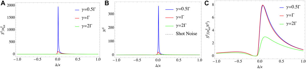
FIGURE 2. (Color online) Frequency responses of the relative signal per photon, noise, and SNR per photon. Parameters in plotting are Δ₁₂ = 0 and J = Γ = 0.1κ. (A) Spectra of the relative signal per photon. The signal reaches the maximum at the resonant point and decreases as the loss γ increases. (B) Spectra of the relative noise. Similar to (A), the noise reaches the maximum at the resonant point and decreases as the loss γ increases. (C) Spectra of SNR per photon. SNR per photon does not reach its maximum value at the resonant point.

FIGURE 3

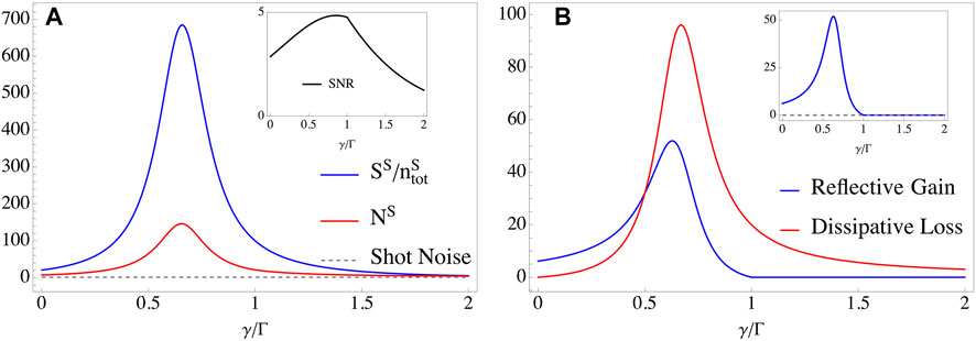
FIGURE 3. (Color online) Relative signal per photon and noise as functions of γ at the resonant point. Parameters in plotting are: Δ = Δ₁₂ = 0, J = Γ = 0.1κ. (A) Both signal (blue line) and noise (red line) experience a process of first increase and then decrease, and reach their maximum value at γ ≃ 0.65Γ, but SNR (black line in inset) reaches the maximum value at γ ≃ 0.85Γ. In addition, the noise N^S is always greater than the shot noise (Gray dotted line). (B) The reflective gain (Blue line, the second term in Eq. 20) and the dissipative loss (Red line, the third term in Eq. 20) as functions of γ with the replacement of matrix $D_Z^S$. Inset: the amplified curves of reflective gain. One can clearly see that it is zero when γ > Γ, because the Heaviside function in Eq. 20 cutoff the parts $|{\tilde{\chi }}_{11}^S-1{|}^2-1<0$.

With the previous results, we now turn to the sensor made up of two giant cavities. In contrast to the case we discussed in the last section, the dissipative matrix D_Z additionally introduces a degree of freedom of the fixed phase ϕ (Δτ is zero at the resonant point), such that the relative signal per photon, noise, and SNR per photon have a response to ϕ, as shown Figure 4 where we also use the same parameters in plotting. Both the signal per photon and the noise experience a process of first increasing and then decreasing as the phase ϕ increases, as shown in Figure 4A,B. An interesting point is that, thanks to the phase ϕ, the output noise can remain at the shot noise level, e.g., N ≃ 1.12 at ϕ = 0.76π when γ = 0.5Γ (Blue line), N ≃ 1.03 at ϕ = 0.84π when γ = Γ (Red line) and N ≃ 1.00 at ϕ = 0.89π when γ = 2Γ (Green line), which are about one order of magnitude smaller than N^S, as shown as the inset in Figure 4B. In Figure 4C, it shows that SNR per photon increases as the loss γ increases when ϕ ∈ [π, 2π], but indeed, SNR per photon reaches its maximum value at γ ≃ 2Γ. ²As we mentioned in the last section, the shot noise is the fundamental limit of the output noise for any sensor. This result also applies to our giant-cavity-based proposal, as shown in Figure 5. The reflective gain and dissipative loss cannot simultaneously be zero although they can be zero by adjusting the phase ϕ, which also explains why the noise is always greater than the shot noise in Figure 4B.

FIGURE 4

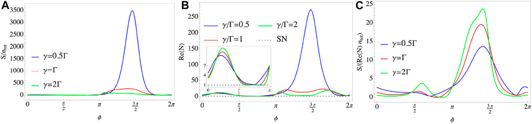
FIGURE 4. (Color online) Relative signal per photon, noise, and SNR per photon as the functions of ϕ at the resonant point. Parameters in plotting are: Δ = Δ₁₂ = 0, J = Γ = 0.1κ. (A) The relative signal as the function of ϕ. As the loss γ increases, the maximum value of the signal decreases; (B) The relative noise as the function of ϕ. The term “SN” is the abbreviation for Shot Noise. Similar to (A), the noise also increases as the loss γ increases, and it is always greater than the shot noise. However, at some certain ϕ, the noise can remain at the shot noise level, e.g., N ≃ 1.12 at ϕ = 0.76π when γ = 0.5Γ, N ≃ 1.03 at ϕ = 0.84π when γ = Γ and N ≃ 1.00 at ϕ = 0.89π when γ = 2Γ. (C) The relative SNR per photon as the function of ϕ. Similar to (A) and (B), SNR per photon also increases as the loss γ increases.

FIGURE 5

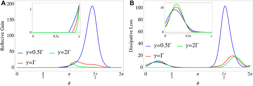
FIGURE 5. (Color online) Reflective gain (A) and dissipative loss (B) as the functions of ϕ. Parameters in plotting are: Δ = Δ₁₂ = 0, J = Γ = 0.1κ. Both reflective gain and dissipative loss can be zero at some certain ϕ but they cannon be zero simultaneously, which is the reason why the noise is always greater than the shot noise in Figure 4B.

A clear comparison with the sensor made up of the small cavities is plotted in Figure 6. As Figure 6A shows, the signal per photon of giant-cavity proposal S/n_tot can be about one order of magnitude greater than that of small-cavity proposal $S^S/n_{\text{tot}}^S$, especially when γ = 2Γ (green line). An interesting point is that Re(N) is almost always smaller than N^S in the entire interval [0, 2π] when γ = Γ, as shown as the red line in Figure 6B. This means that our proposal can effectively decrease the output noise by adjusting the parameter ϕ, compared to Ref. [14]. In addition, from the green and blue lines in Figure 6A,B, one can find that both the ratio of signal per photon $\frac{S}{n_{\text{tot}}}/\frac{S^S}{n_{\text{tot}}^S}$ and the ratio of noise Re(N)/N^S are greater than 1 at some certain values of ϕ, which means both the signal per photon and the noise of the giant-cavity proposal are enhanced compared to the small-cavity proposal. Indeed, this enhancement is led by the non-reciprocal coupling. As we mentioned in Section 2.2, the non-reciprocal coupling means that the cavity 1 can affect the excitation of the cavity 2 via the shared reservoir but not vice-versa, and thus both the signal per photon and the output noise are amplified by this non-reciprocity since the readout waveguide is coupled to the cavity 1. The mathematical reason lies in that the non-reciprocal state transfer matrix $\tilde{\chi }$ effectively amplifies the element ${\tilde{\chi }}_{12}$ but decrease the element ${\tilde{\chi }}_{21}$ when ϕ ≠ (2k + 1)π. Physically, such the amplification and decrease means that the incident photons are transmitted back to cavity 1 rather than stored in cavity 2, with the help of the directional interaction a₂ → a₁. For the signal per photon, this process is equivalent to amplifying the signal S but decreasing the total photon number n_tot; For the output noise Re(N), this process amplifies the dissipative loss. One can examine the above results by substituting Eqs. 25-27 into Eqs. 19, 20. Furthermore, although both the signal S per photon and the output noise Re(N) are enhanced in the interval [π, 1.5π] when γ = 2Γ (green lines in Figure 6A,B, respectively), the SNR per photon is much greater than those with other γ, as shown as the green line in Figure 6C. These results show that the giant-cavity structure is a powerful resource in designing quantum sensors.

FIGURE 6

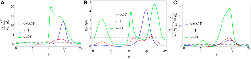
FIGURE 6. (Color online) The ratios of signal per photon (A), output noise (B) and SNR per photon (C) between sensors made up of giant and small cavities. Parameters in plotting are: Δ = Δ₁₂ = 0 and J = Γ = 0.1κ. (A) For some certain intervals, e.g [π, 1.5π], the signals S/n_tot are greater than $S^S/n_{\text{tot}}^S$. Especially, when γ = 2Γ, S/n_tot is about one order of magnitude enhanced compared to $S^S/n_{\text{tot}}^S$. (B) By properly adjusting phase ϕ, Re(N) can be lower than N^S. In particularly, when γ = Γ, Re(N) can be almost smaller than N^S globally. (C) With proper gain and loss, e.g., γ = 2Γ, S/(Re(N)n_tot) is about one order magnitude greater than $S^S/(N^S{n}_{\text{tot}}^S)$. These results show that the giant-cavity structure is a powerful resource in designing quantum sensors.

5 Conclusion and Future Works

In conclusion, we proposed a quantum sensor consisting of two giant cavities. By coupling cavities to a dissipative reservoir at multiple points, a non-reciprocal interaction can be engineered between the cavities and the common reservoir, which requires no non-linear elements. Compared to the standard two-mode quantum sensor [14], the output noise can remain at the shot noise level, which is reduced by about one order of magnitudes. And the signal-to-noise ratio per photon is also enhanced by about one order of magnitude. These results show that the giant-cavity-based sensor can effectively improve sensing precision.

A future direction is to consider how the non-Markovian effect affects the sensing performance. Since we only consider the cases at the resonant point, such that the non-Markovian effect depending on Δτ is neglected. However, this degree of freedom plays important roles in the deep non-Markovian regime τ ≫ 1/κ [35], e.g., it induces a non-exponential decay [37] and a multi-peak excitation spectrum [48]. Therefore, how these non-Markovian effects affect the sensing performance is an open question to be explored in the future, especially when a coherent feedback is applied to control the system [58–62]. A possible method to investigate the influences of the non-Markovian effect is utilizing the quantum simulation platform [63].

Data Availability Statement

The raw data supporting the conclusion of this article will be made available by the authors, without undue reservation.

Author Contributions

YZ and SX conceived the work. SX supervised the project. RW and ZP provided critical comments, suggestions, and text. YZ wrote the first draft of the manuscript. All authors contributed to manuscript revision, read, and approved the submitted version.

Funding

This work was supported by the National Natural Science Foundation of China (NSFC) under Grants 61873162, 61973317, 61833010, 62173201, 12074117 and 12061131011. This work was also supported by the Open Research Project of the State Key Laboratory of Industrial Control Technology, Zhejiang University, China (No. ICT2022B47).

Conflict of Interest

The authors declare that the research was conducted in the absence of any commercial or financial relationships that could be construed as a potential conflict of interest.

Publisher’s Note

All claims expressed in this article are solely those of the authors and do not necessarily represent those of their affiliated organizations, or those of the publisher, the editors, and the reviewers. Any product that may be evaluated in this article, or claim that may be made by its manufacturer, is not guaranteed or endorsed by the publisher.

Acknowledgments

The authors thank Lei Du, Wenlong Li, Qiuyuan Cai, and Sulin Feng for the fruitful discussion.

Footnotes

¹Since the perturbation is small enough, such that it can be expanded as a small quantity and kept to the first order.

²We have simulated SNR with γ ∈ {0.25Γ, 0.5Γ, Γ, 2Γ, 4Γ, 8Γ, 16Γ} and found SNR per photon is maximum at γ = 2Γ. For the sake of keeping the picture simple and clear, we do not show other curves in Figure 4C.

References

1. Schnabel R, Mavalvala N, McClelland DE, Lam PK. Quantum Metrology for Gravitational Wave Astronomy. Nat Commun (2010) 1:121. doi:10.1038/ncomms1122

PubMed Abstract | CrossRef Full Text | Google Scholar

2. Stray B, Lamb A, Kaushik A, Vovrosh J, Rodgers A, Winch J, et al. Quantum Sensing for Gravity Cartography. Nature (2022) 602:590–4. doi:10.1038/s41586-021-04315-3

PubMed Abstract | CrossRef Full Text | Google Scholar

3. Vollmer F, Arnold S, Keng D. Single Virus Detection from the Reactive Shift of a Whispering-Gallery Mode. Proc Natl Acad Sci U.S.A (2008) 105:20701–4. doi:10.1073/pnas.0808988106

PubMed Abstract | CrossRef Full Text | Google Scholar

4. Zhu J, Ozdemir SK, Xiao Y-F, Li L, He L, Chen D-R, et al. On-chip Single Nanoparticle Detection and Sizing by Mode Splitting in an Ultrahigh-Q Microresonator. Nat Photon (2010) 4:46–9. doi:10.1038/nphoton.2009.237

CrossRef Full Text | Google Scholar

5. Zhao N, Hu J-L, Ho S-W, Wan JTK, Liu RB. Atomic-scale Magnetometry of Distant Nuclear Spin Clusters via Nitrogen-Vacancy Spin in diamond. Nat Nanotech (2011) 6:242–6. doi:10.1038/nnano.2011.22

PubMed Abstract | CrossRef Full Text | Google Scholar

6. Shi F, Kong X, Wang P, Kong F, Zhao N, Liu R-B, et al. Sensing and Atomic-Scale Structure Analysis of Single Nuclear-Spin Clusters in diamond. Nat Phys (2014) 10:21–5. doi:10.1038/nphys2814

CrossRef Full Text | Google Scholar

7. Xu X, Chen W, Zhao G, Li Y, Lu C, Yang L. Wireless Whispering-Gallery-Mode Sensor for thermal Sensing and Aerial Mapping. Light Sci Appl (2018) 7:62. doi:10.1038/s41377-018-0063-4

PubMed Abstract | CrossRef Full Text | Google Scholar

8. Sánchez-Burillo E, Duch J, Gómez-Gardeñes J, Zueco D. Quantum Navigation and Ranking in Complex Networks. Sci Rep (2012) 2:605. doi:10.1038/srep00605

PubMed Abstract | CrossRef Full Text | Google Scholar

9. Marks P. Quantum Positioning System Steps in when Gps Fails. New Scientist (2014) 222:19. doi:10.1016/S0262-4079(14)60955-6

CrossRef Full Text | Google Scholar

10. Li B-B, Bulla D, Prakash V, Forstner S, Dehghan-Manshadi A, Rubinsztein-Dunlop H, et al. Invited Article: Scalable High-Sensitivity Optomechanical Magnetometers on a Chip. APL Photon (2018) 3:120806. doi:10.1063/1.5055029

CrossRef Full Text | Google Scholar

11. Li B-B, Bílek J, Hoff UB, Madsen LS, Forstner S, Prakash V, et al. Quantum Enhanced Optomechanical Magnetometry. Optica (2018) 5:850–6. doi:10.1364/OPTICA.5.000850

CrossRef Full Text | Google Scholar

12. Yu C, Janousek J, Sheridan E, McAuslan DL, Rubinsztein-Dunlop H, Lam PK, et al. Optomechanical Magnetometry with a Macroscopic Resonator. Phys Rev Appl (2016) 5:044007. doi:10.1103/PhysRevApplied.5.044007

CrossRef Full Text | Google Scholar

13. Sounas DL, Alù A. Non-reciprocal Photonics Based on Time Modulation. Nat Photon (2017) 11:774–83. doi:10.1038/s41566-017-0051-x

CrossRef Full Text | Google Scholar

14. Lau H-K, Clerk AA. Fundamental Limits and Non-reciprocal Approaches in Non-Hermitian Quantum Sensing. Nat Commun (2018) 9:4320. doi:10.1038/s41467-018-06477-7

PubMed Abstract | CrossRef Full Text | Google Scholar

15. Potton RJ. Reciprocity in Optics. Rep Prog Phys (2004) 67:717–54. doi:10.1088/0034-4885/67/5/r03

CrossRef Full Text | Google Scholar

16. Casimir HBG. On Onsager's Principle of Microscopic Reversibility. Rev Mod Phys (1945) 17:343–50. doi:10.1103/RevModPhys.17.343

CrossRef Full Text | Google Scholar

17. Peng B, Özdemir ŞK, Lei F, Monifi F, Gianfreda M, Long GL, et al. Parity-time-symmetric Whispering-Gallery Microcavities. Nat Phys (2014) 10:394–8. doi:10.1038/nphys432310.1038/nphys2927

CrossRef Full Text | Google Scholar

18. Peng B, Özdemir ŞK, Liertzer M, Chen W, Kramer J, Yılmaz H, et al. Chiral Modes and Directional Lasing at Exceptional Points. Proc Natl Acad Sci U.S.A (2016) 113:6845–50. doi:10.1073/pnas.1603318113

PubMed Abstract | CrossRef Full Text | Google Scholar

19. McDonald A, Clerk AA. Exponentially-enhanced Quantum Sensing with Non-Hermitian Lattice Dynamics. Nat Commun (2020) 11:5382. doi:10.1038/s41467-020-19090-4

PubMed Abstract | CrossRef Full Text | Google Scholar

20. Allen PJ. The Turnstile Circulator. IEEE Trans Microwave Theor Techn. (1956) 4:223–7. doi:10.1109/TMTT.1956.1125066

PubMed Abstract | CrossRef Full Text | Google Scholar

21. Auld BA. The Synthesis of Symmetrical Waveguide Circulators. IEEE Trans Microwave Theor Techn. (1959) 7:238–46. doi:10.1109/TMTT.1959.1124688

CrossRef Full Text | Google Scholar

22. Scalora M, Dowling JP, Bowden CM, Bloemer MJ. The Photonic Band Edge Optical Diode. J Appl Phys (1994) 76:2023–6. doi:10.1063/1.358512

CrossRef Full Text | Google Scholar

23. Tocci MD, Bloemer MJ, Scalora M, Dowling JP, Bowden CM. Thin‐film Nonlinear Optical Diode. Appl Phys Lett (1995) 66:2324–6. doi:10.1063/1.113970

CrossRef Full Text | Google Scholar

24. Konotop VV, Kuzmiak V. Nonreciprocal Frequency Doubler of Electromagnetic Waves Based on a Photonic Crystal. Phys Rev B (2002) 66:235208. doi:10.1103/PhysRevB.66.235208

CrossRef Full Text | Google Scholar

25. Zhukovsky SV, Smirnov AG. All-optical Diode Action in Asymmetric Nonlinear Photonic Multilayers with Perfect Transmission Resonances. Phys Rev A (2011) 83:023818. doi:10.1103/PhysRevA.83.023818

CrossRef Full Text | Google Scholar

26. Abdo B, Sliwa K, Frunzio L, Devoret M. Directional Amplification with a Josephson Circuit. Phys Rev X (2013) 3:031001. doi:10.1103/PhysRevX.3.031001

CrossRef Full Text | Google Scholar

27. Wang D-W, Zhou H-T, Guo M-J, Zhang J-X, Evers J, Zhu S-Y. Optical Diode Made from a Moving Photonic Crystal. Phys Rev Lett (2013) 110:093901. doi:10.1103/PhysRevLett.110.093901

PubMed Abstract | CrossRef Full Text | Google Scholar

28. Abdo B, Sliwa K, Shankar S, Hatridge M, Frunzio L, Schoelkopf R, et al. Josephson Directional Amplifier for Quantum Measurement of Superconducting Circuits. Phys Rev Lett (2014) 112:167701. doi:10.1103/PhysRevLett.112.167701

PubMed Abstract | CrossRef Full Text | Google Scholar

29. Fang K, Luo J, Metelmann A, Matheny MH, Marquardt F, Clerk AA, et al. Generalized Non-reciprocity in an Optomechanical Circuit via Synthetic Magnetism and Reservoir Engineering. Nat Phys (2017) 13:465–71. doi:10.1038/nphys4009

CrossRef Full Text | Google Scholar

30. Xu Q, Schmidt B, Pradhan S, Lipson M. Micrometre-scale Silicon Electro-Optic Modulator. Nature (2005) 435:325–7. doi:10.1038/nature03569

PubMed Abstract | CrossRef Full Text | Google Scholar

31. Phare CT, Daniel Lee Y-H, Cardenas J, Lipson M. Graphene Electro-Optic Modulator with 30 GHz Bandwidth. Nat Photon (2015) 9:511–4. doi:10.1038/nphoton.2015.122

CrossRef Full Text | Google Scholar

32. Kockum AF, Delsing P, Johansson G. Designing Frequency-dependent Relaxation Rates and Lamb Shifts for a Giant Artificial Atom. Phys Rev A (2014) 90:013837. doi:10.1103/PhysRevA.90.013837

CrossRef Full Text | Google Scholar

33. Schuetz MJA, Kessler EM, Giedke G, Vandersypen LMK, Lukin MD, Cirac JI. Universal Quantum Transducers Based on Surface Acoustic Waves. Phys Rev X (2015) 5:031031. doi:10.1103/PhysRevX.5.031031

CrossRef Full Text | Google Scholar

34. Manenti R, Kockum AF, Patterson A, Behrle T, Rahamim J, Tancredi G, et al. Circuit Quantum Acoustodynamics with Surface Acoustic Waves. Nat Commun (2017) 8:975. doi:10.1038/s41467-017-01063-9

PubMed Abstract | CrossRef Full Text | Google Scholar

35. Guo L, Grimsmo A, Kockum AF, Pletyukhov M, Johansson G. Giant Acoustic Atom: A Single Quantum System with a Deterministic Time Delay. Phys Rev A (2017) 95:053821. doi:10.1103/PhysRevA.95.053821

CrossRef Full Text | Google Scholar

36. Kockum AF, Johansson G, Nori F. Decoherence-free Interaction between Giant Atoms in Waveguide Quantum Electrodynamics. Phys Rev Lett (2018) 120:140404. doi:10.1103/physrevlett.120.140404

PubMed Abstract | CrossRef Full Text | Google Scholar

37. Andersson G, Suri B, Guo L, Aref T, Delsing P. Non-exponential Decay of a Giant Artificial Atom. Nat Phys (2019) 15:1123–7. doi:10.1038/s41567-019-0605-6

CrossRef Full Text | Google Scholar

38. Ekström MK, Aref T, Ask A, Andersson G, Suri B, Sanada H, et al. Towards Phonon Routing: Controlling Propagating Acoustic Waves in the Quantum Regime. New J Phys (2019) 21:123013. doi:10.1088/1367-2630/ab5ca5

CrossRef Full Text | Google Scholar

39. Delsing P, Cleland AN, Schuetz MJA, Knörzer J, Giedke G, Cirac JI, et al. The 2019 Surface Acoustic Waves Roadmap. J Phys D: Appl Phys (2019) 52:353001. doi:10.1088/1361-6463/ab1b04

CrossRef Full Text | Google Scholar

40. Kannan B, Ruckriegel MJ, Campbell DL, Kockum AF, Braumüller J, Kim DK, et al. Waveguide Quantum Electrodynamics with Superconducting Artificial Giant Atoms. Nature (2020) 583:775–9. doi:10.1038/s41586-020-2529-9

PubMed Abstract | CrossRef Full Text | Google Scholar

41. Kockum AF. Quantum Optics with Giant Atoms-The First Five Years. In: International Symposium on Mathematics, Quantum Theory, and Cryptography. Singapore: Springer (2021). p. 125–46. doi:10.1007/978-981-15-5191-8_12

CrossRef Full Text | Google Scholar

42. Guo L, Kockum AF, Marquardt F, Johansson G. Oscillating Bound States for a Giant Atom. Phys Rev Res (2020) 2:043014. doi:10.1103/PhysRevResearch.2.043014

CrossRef Full Text | Google Scholar

43. Vadiraj AM, Ask A, McConkey TG, Nsanzineza I, Chang CWS, Kockum AF, et al. Engineering the Level Structure of a Giant Artificial Atom in Waveguide Quantum Electrodynamics. Phys Rev A (2021) 103:023710. doi:10.1103/PhysRevA.103.023710

CrossRef Full Text | Google Scholar

44. Du L, Cai M-R, Wu J-H, Wang Z, Li Y. Single-photon Nonreciprocal Excitation Transfer with Non-Markovian Retarded Effects. Phys Rev A (2021) 103:053701. doi:10.1103/PhysRevA.103.053701

CrossRef Full Text | Google Scholar

45. Du L, Li Y. Single-photon Frequency Conversion via a Giant Λ -type Atom. Phys Rev A (2021) 104:023712. doi:10.1103/PhysRevA.104.023712

CrossRef Full Text | Google Scholar

46. Du L, Zhang Y, Wu J-H, Kockum AF, Li Y. Giant Atoms in Synthetic Frequency Dimensions. arXiv: 2111.05584 (2021).

Google Scholar

47. Cai QY, Jia WZ. Coherent Single-Photon Scattering Spectra for a Giant-Atom Waveguide-QED System beyond the Dipole Approximation. Phys Rev A (2021) 104:033710. doi:10.1103/PhysRevA.104.033710

CrossRef Full Text | Google Scholar

48. Zhu Y, Wu R, Xue S. Spatial Non-Locality Induced Non-Markovian EIT in a Single Giant Atom. arXiv: 2106.05020 (2021).

Google Scholar

49. Pezzè L, Smerzi A, Oberthaler MK, Schmied R, Treutlein P. Quantum Metrology with Nonclassical States of Atomic Ensembles. Rev Mod Phys (2018) 90:035005. doi:10.1103/RevModPhys.90.035005

CrossRef Full Text | Google Scholar

50. Degen CL, Reinhard F, Cappellaro P. Quantum Sensing. Rev Mod Phys (2017) 89:035002. doi:10.1103/RevModPhys.89.035002

CrossRef Full Text | Google Scholar

51. Bao L, Qi B, Dong D, Nori F. Fundamental Limits for Reciprocal and Nonreciprocal Non-Hermitian Quantum Sensing. Phys Rev A (2021) 103:042418. doi:10.1103/PhysRevA.103.042418

CrossRef Full Text | Google Scholar

52. Shen J-T, Fan S. Theory of Single-Photon Transport in a Single-Mode Waveguide. I. Coupling to a Cavity Containing a Two-Level Atom. Phys Rev A (2009) 79:023837. doi:10.1103/PhysRevA.79.023837

CrossRef Full Text | Google Scholar

53. Zhu YT, Jia WZ. Single-photon Quantum Router in the Microwave Regime Utilizing Double Superconducting Resonators with Tunable Coupling. Phys Rev A (2019) 99:063815. doi:10.1103/PhysRevA.99.063815

CrossRef Full Text | Google Scholar

54. Clerk AA, Devoret MH, Girvin SM, Marquardt F, Schoelkopf RJ. Introduction to Quantum Noise, Measurement, and Amplification. Rev Mod Phys (2010) 82:1155–208. doi:10.1103/RevModPhys.82.1155

CrossRef Full Text | Google Scholar

55. Huang S, Agarwal GS. Reactive-coupling-induced normal Mode Splittings in Microdisk Resonators Coupled to Waveguides. Phys Rev A (2010) 81:053810. doi:10.1103/PhysRevA.81.053810

CrossRef Full Text | Google Scholar

56. Qu K, Agarwal GS. Phonon-mediated Electromagnetically Induced Absorption in Hybrid Opto-Electromechanical Systems. Phys Rev A (2013) 87:031802. doi:10.1103/PhysRevA.87.031802

CrossRef Full Text | Google Scholar

57. Weis S, Rivière R, Deléglise S, Gavartin E, Arcizet O, Schliesser A, et al. Optomechanically Induced Transparency. Science (2010) 330:1520–3. doi:10.1126/science.1195596

PubMed Abstract | CrossRef Full Text | Google Scholar

58. Xue S-B, Wu R-B, Zhang W-M, Zhang J, Li C-W, Tarn T-J. Decoherence Suppression via Non-Markovian Coherent Feedback Control. Phys Rev A (2012) 86:052304. doi:10.1103/PhysRevA.86.052304

CrossRef Full Text | Google Scholar

59. Xue S, Petersen IR. Realizing the Dynamics of a Non-Markovian Quantum System by Markovian Coupled Oscillators: a Green's Function-Based Root Locus Approach. Quan Inf Process (2016) 15:1001–18. doi:10.1007/s11128-015-1196-5

CrossRef Full Text | Google Scholar

60. Xue S, Wu R, Hush MR, Tarn T-J. Non-Markovian Coherent Feedback Control of Quantum Dot Systems. Quan Sci. Technol. (2017) 2:014002. doi:10.1088/2058-9565/aa6125

CrossRef Full Text | Google Scholar

61. Xue S, Hush MR, Petersen IR. Feedback Tracking Control of Non-Markovian Quantum Systems. IEEE Trans Contr Syst Technol (2017) 25:1552–63. doi:10.1109/TCST.2016.2614834

CrossRef Full Text | Google Scholar

62. Xue S, Nguyen T, James MR, Shabani A, Ugrinovskii V, Petersen IR. Modeling for Non-Markovian Quantum Systems. IEEE Trans Contr Syst Technol (2020) 28:2564–71. doi:10.1109/TCST.2019.2935421

CrossRef Full Text | Google Scholar

63. Chen X-Y, Zhang N-N, He W-T, Kong X-Y, Tao M-J, Deng F-G, et al. Global Correlation and Local Information Flows in Controllable Non-Markovian Open Quantum Dynamics. Npj Quan Inf (2022) 8:22. doi:10.1038/s41534-022-00537-z

CrossRef Full Text | Google Scholar