
95% of researchers rate our articles as excellent or good
Learn more about the work of our research integrity team to safeguard the quality of each article we publish.
Find out more
ORIGINAL RESEARCH article
Front. Phys. , 16 June 2022
Sec. Quantum Engineering and Technology
Volume 10 - 2022 | https://doi.org/10.3389/fphy.2022.896174
This article is part of the Research Topic Quantum Light for Imaging, Sensing and Spectroscopy View all 11 articles
 R. Gutiérrez-Jáuregui1*
 R. Jáuregui2*
Atomic gases tightly trapped near the focus of an electromagnetic wave interact with photons that exhibit a complex structure, displaying strong gradients of field amplitude and local polarization that can lead to topological phase singularities. We illustrate the consequences of this structure on a paradigmatic nonlinear optical process: three-wave mixing. The process begins by proper selection of the pump field, whose spatial structure is tailored to present huge gradients of the EM field that enhance atomic excitations through forbidden transitions. Atoms can then be depopulated via two electric dipole decays in a cascade configuration, thus providing the three necessary waves. The properties of the down-converted photons are conditioned to those of the pump field through phase matching conditions. It is emphasized that the expression of the photons must incorporate both the structure of the vectorial EM modes and the spatial configuration of the atomic trap. Due to the three-dimensional focusing, the slowly varying envelope approximation becomes inadequate when describing the scattered EM field. We discuss an alternative using a Green function formalism valid for any configuration of the field that also allows to identify the phase matching conditions. Spherical vectorial waves exemplify most concepts here discussed, including the possibility of observing nonlinear quantum phenomena at the single photon level.
It is now 60 years from publication of the emblematic work: Interaction between light waves in a nonlinear dielectric where Bloembergen and collaborators set out to connect the radiative response of electrons in atomic gases to the nonlinear optical properties of macroscopic dielectrics [1]. The connection was based on the collective, coherent scattering of light from atoms inside the gas and its relation to the incident electromagnetic field. The authors showed that the coherence between scattered and incident fields induces electric moments on the atoms that can yield nonlinear terms in the field strength, thus coupling waves of different frequencies. To unearth these effects a quasimonochromatic light source of high-brightness, directionality, and stable intensity as that given by the laser was required [1]. As modern technologies delve deeper into miniaturization, we need to look back at this connection but now placing emphasis on an efficient transfer of light at low intensities. An efficiency that can be reached by tailoring spatial and temporal profiles of light and matter through light-shaping techniques [2] and versatile atomic traps [3, 4].
Considered most broadly, the nonlinear process arises from the underlying interaction between light and matter. An illuminated atom probes and modifies the surrounding electromagnetic (EM) field, acquiring information on field intensities, gradients, and temporal correlations as it scatters photons between populated and vacuum modes. When the illuminating field is tailored to match the spatial and temporal profiles of the atomic radiation pattern, it can create a strong nonlinear response. Three-wave mixing represents the most simple response where fields of different frequencies couple and the potential of structured light is made apparent. Its implementation requires for three waves to induce a cycling transition in an atomic medium: moving up via, for instance, an electric quadrupole transition and cascading down via two electric dipole transitions through an intermediate level. Under adequate phase matching conditions an incident beam inducing the quadrupole transition gives rise to lower frequency waves, thus acting as a parametric amplifier. This example was chosen in Ref. [1] to show how symmetry constraints affect the nonlinear coupling. The experimental challenges to induce this process in atomic gases at the time were, however, formidable, with the conditions for observing quadrupole transitions being found in astrophysical or laboratory plasmas mostly [5]. Experiments searching to create correlated photons whose frequencies matched the atomic transition moved towards next order [1]. The first sources of correlated photon pairs were based on a cascade decay in a four-wave mixing process [6, 7] and led to enabling technologies in lithography [8], tomography [9], cryptography [10] and imaging [11, 12] with multiple physics [13] and transdisciplinary [14, 15] applications.
Atomic electric quadrupole transitions require large gradients in the amplitude of the incoming field. It is now possible to meet the experimental challenges to induce these transitions and explore three-wave mixing in atomic gases. On the one hand, further development of high-intensity lasers allows for the observation of quadrupole transitions even using thermal atomic samples and paraxial pump beams [16–18]. On the other hand, a quadrupole transition can be induced by large gradients in the amplitude of the incident EM field down to the limit of weak intensities. For this, spatial gradients are generated by shaping light using either phase singularities [19, 20] or evanescent waves [21] for which even micro-Watt intensity lasers can suffice [22].
In this manuscript we look back at the three-wave mixing process following ideas of light shaping and monitoring mechanisms that have been developed since the early days of nonlinear optics. Deep down this work is driven by the following thought: transitions with a single photon can trigger strong nonlinear optical processes when the spatial profile of the photon is tailored. The ideal scenario involves spherical vectorial waves, whose implementation remains challenging as they require control of the full 4π angle surrounding the atom. There are, however, experimental platforms where this control is achieved to a good approximation. In particular a single ion trapped at the focus of a parabolic mirror [23, 24] is a feasible set-up for achieving nonlinear strong coupling between few photons associated to vectorial modes. It has already been shown that a single photon can induce an electric dipole transition with high-probability in this set-up due to the similarities between parabolic and spherical waves [25]. Here, we study a three-wave mixing process based on ideal spherical vectorial modes [26]. We consider tightly trapped atoms in the Lamb-Dicke regime where the spatial confinement approaches the typical transition wavelengths. Through this ideal scenario we identify the theoretical tools necessary to understand the nonlinear process in detail, and establish a route to perform theoretical and experimental realizations of nonlinear optics events with a minimum number of photons.
The manuscript is organized as follow. In Section 1 we introduce our model where a tightly trapped atom is coupled to a structured EM field. Emphasis is placed on the vectorial structure of the field and effects related to the spatial extent of the trap on the atom-light coupling. We show that the trap strength can alter the atomic multipole decay rates through a form factor. At the end of this Section we revisit spherical vectorial waves and their relevance for the system under study. Section 2 concerns the connection between atomic transitions and nonlinear optics. We consider the specific example of an atom in a cascade configuration driven via an electric quadrupole transition by an incoming spherical wave. The nonlinear susceptibilities and collective responses of atomic systems are worked out for tightly trapped atoms. The mesoscopic densities of electric dipole and quadrupole polarization as sources of scattered photons are discussed. In Section 3 we introduce a dyadic Green function formalism that can be used to overcome the theoretical challenges that rise for deeply focused modes, such as, non-applicability of the slowly varying envelope approximation and the identification of the phase matching conditions. We conclude in Section 4 with a recapitulation of our results and the scope of our analyses.
We consider an atomic gas coupled to a free electromagnetic field. The dynamics of this composite system are given by the Hamiltonian
where
The gas is assumed to be tightly trapped and formed by atoms with three relevant electronic states |s⟩(s = a, b, c) in a cascade configuration sketched in Figure 1. It is described by the Hamiltonian
where the operator
with
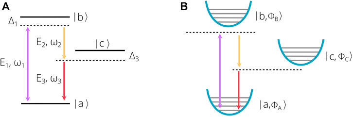
FIGURE 1. (A) A three-level atom mediates the interaction between different waves. It is considered to be excited via a quadrupole transition connecting levels |a⟩ and |b⟩ and decays through cascade dipole transitions along level |c⟩. (B) Since the atomic system is trapped in a region comparable to the involved radiative wavelengths, vibrational motion effects must be included.
It is convenient to write the mode amplitudes Eγ inside a restricted Fourier space where the free-space dispersion relation |k|2 = ω2/c2 has been imposed. In this space the amplitudes are
with dΩk a solid angle element and fγ the angular spectrum of the mode. Equation 6 gives a direct connection between plane waves and general structured modes.
The interaction between atom and field supports a multipole description due to the small size of the atom as compared to the wavelengths involved in most radiative transitions [27]. For extremely 3D-focused structured light, large gradients of the field amplitude and spatial-dependent polarization are found [28]. If the atom is trapped nearby the focus of the light mode it is necessary to move beyond the dipole approximation, done here through an interaction Hamiltonian
written in terms of the atomic electric dipole
Equation 7 illustrates how an atom probes an electromagnetic field by correlating its internal states to the state of the field. Through the electric and magnetic dipole moments it probes local field amplitudes and quadratures, through the quadrupole moment it gains information of spatial gradients of the field. By moving past the dipole moment it is possible to acquire a better landscape of the EM field. Furthermore, the theoretical tools used to describe this extended landscape resemble those commonly used under the dipole approximation. The similarity is made transparent by inserting Eq. 4 into Eq. 7 and applying the rotating-wave approximation, such that—in a reference frame oscillating with
where
The contributions read explicitly as
Here, the matrix elements
From Eq. 7 it is possible to obtain Rabi oscillations, decay rates, and radiative shifts caused by higher multipole terms following standard techniques used in quantum optics. There is, however, a difference that has to be emphasized. The coupling depends on the trapping strength through the operator
plus two analogue terms for the magnetic dipole and electric quadrupole moments. With vibrational states defining the strength at which EM field an atom interact, a natural question is raised: Is it possible to alter the decay rate of an atom in an structured environment by changing the location and strength of the trap? While the effect of the location has been studied at length in the past, where tests of the Purcell enhancement factor depend on the location of an atom with respect to a boundary that alters the field distribution [29], the effect of trap strength is less explored. We answer this question in the affirmative below, where we show that for localized environments the spontaneous decay rate can be reduced (enhanced) for weaker (tighter) traps. The change is attributed to the extension of the atomic trap, which leads to an average over regions where field intensity and gradient change.
To describe the spontaneous emission of an atomic gas inside a structured environment, we consider the probability that an excited atom emits a photon into a free mode during a time interval τ. From Eq. 8 the probability for this process to occur, regardless of the final vibrational state, is given by the integral
thus posing frequency missmatch conditions on the modes the atom interacts most strongly with. In general these conditions depend on a vibrational shift ωAB, but, when the electronic transition frequency is much larger than the relevant CM transition frequencies ωss′ ≫ ωAB, this shift can be neglected [30]. By removing these shifts from the equation the states |ΦB⟩ can be averaged out using the completeness of the vibrational states, leading to
with
Equation 13 should be read as a probability distribution that weights the decay process. The atom interacts with many modes of the environment such that the spontaneous decay rates is obtained from the sum
consistent with the Born and Markov approximations. By removing the correlations that build-up between field and atom we have made the Born approximation, and by extending the time integral without accounting for selfconsistent exchanges we have performed the Markov approximation. In this sense, the spread ωss + ωAB introduced by vibrational states has to be much smaller than the free mode density in order to be neglected. This is usually achieved in free space, and is a good approximation to half cavities where modes acquire a linewidth.
It is now possible to identify the decay rate of an atom inside an structured environment. The transition rates between electronic states incorporate information about the spatial region explored by the atom and the vectorial nature of the radiated field. By using the angular spectrum of the field defined in Eq. 6 the spontaneous rates are found to be [25].
where we have used square brackets [x]σ to denote the σ component of vectors and tensors and adopted the circular polarization basis {eσ} = {e± = ex ± iey, e0 = ez}. The contribution of each mode becomes
The effect of the vibrational states for all multiple moments is given entirely by a form factor
The form factor shows that the center-of-mass motion performs an average over the field distributions. The average depends on the atomic center of mass initial state. For an atom prepared in the ground state of an harmonic trap with angular frequency components Λx,y,z centered at the position X0—which does not need to coincide with the origin used to describe the EM field—the form factor is
The average carries information on the trap through the Lamb-Dicke parameters
Through Eqs 15a, 15b, 15c, 16a, 16b, 16c, Eq. 17 we have shown that decay rates depend on the EM mode density evaluated at the atomic resonance frequency and also on the average value determined by the vibrational states. The electromagnetic modes γ that participate in Eqs 15a, 15b, 15c can be constrained by imposing physical boundaries, as done in experiments with optical cavities. Then, the enhancement [29] or inhibition [35, 36] of the spontaneous emission rate depends on the electromagnetic structure of the environment and the location and trapping strength of the atom. Notice that this control is expected not only for electric dipole transitions, but for any multipole transition as we have just illustrated for electric quadrupole and magnetic dipole cases.
It is worth mentioning that for atoms in free-space the EM field is homogeneous and the dipolar and quadrupolar spontaneous emission decay rates are
This can be shown by evaluating the
for each polarization, and using the completeness relation of polarizations ϵk,λ and wavevectors k. For a systematic approach beyond the quadrupolar interaction, however, it is more convenient to use the spherical modes.
The structure of the radiated field incorporates the atomic symmetries that arise from the central field model. In the mean field scheme, individual radiative electronic transitions involve a single electron that changes its orbital and yields a non-null electromagnetic multipole for the atom as a whole. An EM multipole transition of an atom can be either described as the emission or absorption of a single photon in an appropriate spherical vectorial mode, or as divided along multiple photon channels with wavevectors k and specific angular distribution probabilities. Spherical vectorial modes then lead to a more efficient transfer than their wavevector counterparts.
This efficient transfer is already suggested by the form of the spherical vectorial modes. In free space a monochromatic spherical wave of frequency ω and amplitude
The spectrum describes the coupling of orbital and polarization angular momenta of photons to yield a total angular momentum {jm} as described by the functions
The radiative transitions that connect two-atomic states are ruled by strict conservation laws for energy, linear momentum, and angular momentum of the atom-radiation system as a whole. These conservation laws are naturally satisfied by spherical modes where electric and magnetic multipole transitions involve a single
with jj(kr) the spherical Bessel functions with k = ω/c and the position r = {r, θ, ϕ}. This form was used to obtain the radiative decay of Eqs 19a, 19b, 19c, but, by portraying the wave as a single vectorial mode, there is no need to account for the contribution of each wavevector and polarization. Similar descriptions are found for the spherical electric modes. Relevant, well-known mathematical properties of spherical vectorial modes are summarized in Supplementary Appendix SAI including a connection to vectorial plane waves. We show explicitly the simple structure of the modes in k-space that is used to define a scalar product from which the EM field can be quantized. These properties emphasize that the mode structure results from the direct coupling of orbital and polarization angular momenta of the field.
Figures 2–4 are used to illustrate the rich spatial patterns of vectorial modes. In an effort to show the symmetries involved, isointensity surfaces are drawn for each polarization e±,0, and for the total intensity of the spherical waves. As anticipated in the Introduction, the polarization and configuration structure in this subwavelength region is complex. High gradients of the intensity and vortices along a dislocation line for certain polarizations can be found as shown by the phase structure in the XY plane.
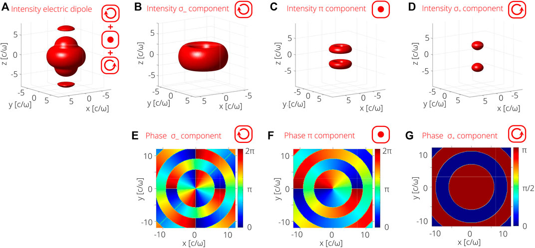
FIGURE 2. Isosurfaces of an electric dipole
We begin with Figure 2 where each polarization component of the electric dipole spherical wave is described by a combination of spherical functions Yℓm with ℓ = 0 and 2, as we now discuss. Figure 2 shows the
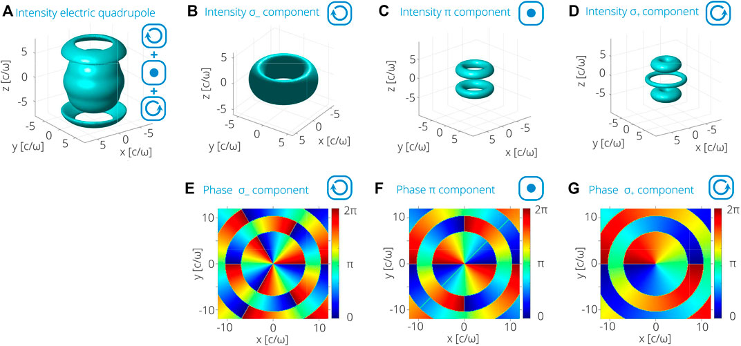
FIGURE 3. Isosurfaces of an electric quadrupole
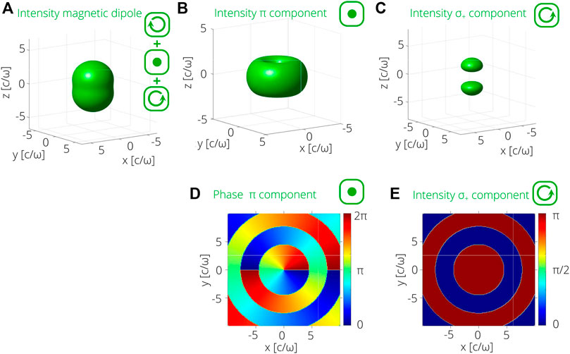
FIGURE 4. Isosurfaces of an magnetic dipole
The results are to be compared with standard paraxial optics. For paraxial optics, light polarization is approximately a global concept. There is a main direction of propagation and the polarization vectors are approximately perpendicular to it. This facilitates the identification of processes where only either σ+, σ− or π transitions occur; π-transitions require a main direction of propagation perpendicular to a quantization-axis defined by the environment as mentioned in the beginning of this Subsection. For each type of transition the atomic internal states experience a change of the internal magnetic number Δm = 1, −1, 0 respectively. If a realization of a few atomic levels model is desired, a search of an atomic- EM field configuration is performed to maximize the relevance of predetermined internal atomic sublevels that participate in the nonlinear optical process.
Having described how light can be tailored to induce particular transitions with high probability, we now move to the nonlinear response of an atomic gas. For this we are going to consider the case drawn in Figure 1 where a three-level atomic gas is driven by a structured EM mode. States |a⟩ and |b⟩ are connected through two paths: one via a quadrupole transition with moment qab; and the other via two electric dipole transitions through an intermediate level |c⟩ with moments dac and dbc. All other moments are considered negligible. The incident mode
Three-wave mixing relies on the coherent scattering from mode
where we separated the three EM modes
naturally divides into free and scattered components. The electromagnetic
where ρCM describes the vibrational motion of the atom and ρ describes its electronic state. This form requires that center of mass and internal states are not correlated at an initial time, and remain so throughout the nonlinear process. This condition could be valid in the Lamb-Dicke regime. From Eqs 23, 24 dipole and quadrupole moment densities P and Q of the three-level atomic gas can be defined as
where the total number of trapped atoms N is first introduced.
Non-linearities enter the picture through the internal state of the atom. They result from the participation of photons inside γ modes at different orders in the coupling strength κ
The series converges for κ lower than the detunings Δ and decay rates Γ(mult). Three-wave mixing appears at second order in the series, the details are described in the Supplementary Appendix SAII following a semiclassical approach equivalent to an adiabatic elimination of the atomic variables in the fully quantum regime [39]. The final expression for the atomic polarization at a position X is
where the leading terms are shown to be
Meanwhile, the quadrupole densities oscillate as
Once the electronic states are adiabatically eliminated, the field evolution of Eq. 23 is equivalent to an effective Hamiltonian density of the atomic gas interacting with the EM field
Here, the summation is performed over free modes γi whose frequency ωi close to the transition frequency ωss′ and their polarization and angular momentum jimi are adequate to induce the atomic transition with the corresponding multipole moment. That is, rapidly oscillating terms derived from far from resonance conditions or an spatial configuration out of the expected spherical vector mode one have been discarded.
Having revisited the connection between electronic processes and nonlinear optical processes, we can now exploit the connection to Maxwell equations. For localized sources which admit an efficient multipole expansion, the radiated field operator
where the sources
divide into electric dipole
It is possible to extend the formalism to include magnetic dipole transitions through a magnetization term
In our case, Eq. 32 stems from the interaction Hamiltonian beyond the dipole approximation written in Eq. 7 and the decomposition of the electric fields [4]. The form of the interaction led naturally to the vectorial spherical waves associated to each atomic radiative transition and then to source terms of this form. The particular atomic evolution follows from a master equation evolution (as defined in Supplementary Appendix SAII), but the form is universal.
Note that radiation can also be generated by so-called “free” sources. An example is radiation scattered by structureless ideal charges such as electrons, i.e., the Compton effect, which has frequently been described using a plane wave expansion of the quantized EM field [31]. Recent theoretical studies concern the Compton effect with photons associated to structured beams [41], and the implementation of the inverse Compton effect for twisted electron beams is an active area of research [42].
For the three-wave mixing process considered here, the induced moments oscillate at frequencies ω1, ω2 and ω3. As such, the evolution of the field amplitudes can be decomposed into a Fourier series that leads to
whenever the temporal phase matching condition is imposed ω1 = ω2 + ω3. From them, conditions yielding a high efficiency of parametric processes based on atomic coherence can be obtained [43]. Note that the full quantum treatment implicit in Eq. 32 allows to study correlations of the quadrature equations of the EM modes, including squeezing conditions [44].
Most implementations of nonlinear optics processes consider input paraxial beams driving the atomic gas. The set of paraxial modes
Schwinger [46] introduced an elegant formalism to evaluate the response function between the electromagnetic field and a polarization source using the Green function dyadic. As Maxwell equation, Eq. 32, can be worked out using this formalism for generalized multipole sources we now revisit this formalism.
The Green dyadic Γ is a tensor with r, s components
with
Where the free field
For a retarded scheme and a vectorial spherical expansion of the electric field operators in free space, the tensor is decomposed as
with jℓ and
We can now use this formalism to describe the phase matching conditions that rule the underlying nonlinear processes. For plane waves phase matching conditions establish the relations between the wave vectors of the involved EM modes that guarantee the highest efficiency of an optical nonlinear process. In the quantum realm, these equations are interpreted as the conservation of linear momentum of the participating photons. For a homogeneous atomic gas, the three-wave mixing phase matching conditions are
For beams exhibiting a common dislocation line—and correspondingly a non-trivial local orbital momentum along that line—the phase matching conditions correlate the topological charge of the vortices so that the angular momentum of the photons is conserved [47, 48]. For an isotropic atomic sample and for modes exhibiting optical vortices of topological charge mi along a common axes, for our process
In this Section we show how they naturally emerge from the dyadic treatment of the scattered field. To that end it is just necessary the integrate the Maxwell Equation Eqs 38a, 38b over the spatial variables of the localized source
If the 3D sample is in an isotropic trap, the angular integration acquires an analytic expression (some formulae useful for the calculation of the spatial derivatives of the spherical waves can be found in the Supplementary Appendix SAI). The integrals are, in general, a linear combination of the Wigner 3-j symbols
available in most numerical platforms. The phase matching conditions result from the identification of non-null Wigner 3-j symbols,
These phase matching conditions can be interpreted as a conservation of the total angular momentum and not just its z-component for the photons involved in the three-wave mixing process.
Since just a constrained set of γpm modes satifies the phase matching conditions, the scattered field is given by
An advantage of working with spherical vectorial modes is that any set of three modes γab, γbc and γca with ω1 = ω2 + ω3 must be considered as usual, but the phase angular matching conditions select a discrete set of few modes specified by the polarization P and the jss′ and mss′ values that satisfy the angular phase matching conditions. This is a basic difference with standard studies where the spatial phase matching is satisfied by a continuous set of spatial modes.
Once few of these modes are identified one could now apply, e.g., the semiclassical approximation or other standard techniques [49–51] to work out the behavior of the quantum quadratures of the field and their correlation to the atomic degrees of freedom. The modes, of course, depend on the experimental conditions.
We have presented a description of three-wave mixing inside an atomic cloud. We began by showing how this process could be efficiently induced by properly shaping the light field and then moved to the description of the free and scattered field that are ultimately measured in an experiment. For this, we went beyond the dipole approximation and showed that the system is naturally described by multipole spherical waves. Multipole spherical waves yield the optimal description of the basic radiative atomic processes. As such, they are paradigmatic structured light fields. Yet, their use in the description of nonlinear systems is scarse. The reason is that most implementations of nonlinear processes employ laser beams and assume a paraxial regime. Nowadays technological developments go in a different direction. Optimal coupling to minimize energy costs in, e.g., quantum information protocols require the realization of nonlinear processes triggered by single photons [52]. A natural scheme to achieve such a coupling is by trapping atoms nearby the focus of spherical vectorial waves.
The main task in this work was to emphasize both the effects of trapping on the radiative responses of an atom and present a way to surmount the difficulties that arise. These included moving beyond dipolar approximation, and the breakdown of commonly used approximations as the slowly varying envelope one. We showed how the dyadic Green function formalism is easily implemented and allows for the identification of a discrete set of modes that would participate in the nonlinear process once the relevant atomic states are identified.
The calculations were described by a paradigmatic process that can now be reached in experiments with atomic gases: three-wave mixing. Notice, however, that the general concepts introduced in our work can be extended to any nonlinear process. In addition the dyadic formalism can be directly applied for other symmetries; yielding a direct route for the identication of the phase matching condition. While standard techniques were developed with dipolar transitions and plane waves in mind, the extension to structured light can be readily done with the appropriate basis in mind.
The original contributions presented in the study are included in the article/Supplementary Material, further inquiries can be directed to the corresponding authors.
RG-J and RJ contributed with conceptual ideas, methodology strategies and writing of the manuscript.
This work was partially supported by PAPIIT-DGAPA-UNAM IN-103020. RG-J acknowledges financial support by the National Science Foundation QII-TAQS (Award No. 1936359).
The authors declare that the research was conducted in the absence of any commercial or financial relationships that could be construed as a potential conflict of interest.
All claims expressed in this article are solely those of the authors and do not necessarily represent those of their affiliated organizations, or those of the publisher, the editors and the reviewers. Any product that may be evaluated in this article, or claim that may be made by its manufacturer, is not guaranteed or endorsed by the publisher.
The Supplementary Material for this article can be found online at: https://www.frontiersin.org/articles/10.3389/fphy.2022.896174/full#supplementary-material
1. Armstrong JA, Bloembergen N, Ducuing J, Pershan PS. Interactions Between Light Waves in a Nonlinear Dielectric. Phys Rev (1962) 127:1918–39. doi:10.1103/physrev.127.1918
2. Rubinsztein-Dunlop H, Forbes A, Berry MV, Dennis MR, Andrews DL, Mansuripur M, et al. Roadmap on Structured Light. J Opt (2016) 19:013001. doi:10.1088/2040-8978/19/1/013001
3. Monroe C, Campbell WC, Duan LM, Gong ZX, Gorshkov AV, Hess PW, et al. Programmable Quantum Simulations of Spin Systems with Trapped Ions. Rev Mod Phys (2021) 93:025001. doi:10.1103/revmodphys.93.025001
4. Navon N, Smith RP, Hadzibabic Z. Quantum Gases in Optical Boxes. Nat Phys (2021) 17:1334–41. doi:10.1038/s41567-021-01403-z
5. Biémont E, Zeippen CJ. Probabilities for Forbidden Transitions in Atoms and Ions: 1989-1995. A Commented Bibliography. Phys Scr (1996) T65:192–7. doi:10.1088/0031-8949/1996/t65/029
6. Fry ES. Two-Photon Correlations in Atomic Transitions. Phys Rev A (1973) 8:1219–32. doi:10.1103/physreva.8.1219
7. Aspect A, Grangier P, Roger G. Experimental Realization of Einstein-Podolsky-Rosen-Bohm Gedankenexperiment: A New Violation of Bell's Inequalities. Phys Rev Lett (1982) 49:91–4. doi:10.1103/physrevlett.49.91
8. D’Angelo M, Chekhova MV, Shih Y. Two-Photon Diffraction and Quantum Lithography. Phys Rev Lett (2001) 87:013602.
9. Nasr MB, Saleh BE, Sergienko AV, Teich MC. Demonstration of Dispersion-Canceled Quantum-Optical Coherence Tomography. Phys Rev Lett (2003) 91:083601. doi:10.1103/PhysRevLett.91.083601
10. Gisin N, Ribordy G, Tittel W, Zbinden H. Quantum Cryptography. Rev Mod Phys (2002) 74:145–95. doi:10.1103/revmodphys.74.145
11. Pittman TB, Shih YH, Strekalov DV, Sergienko AV. Optical Imaging by Means of Two-Photon Quantum Entanglement. Phys Rev A (1995) 52:R3429–R3432. doi:10.1103/physreva.52.r3429
12. Pepe FV, Di Lena F, Mazzilli A, Edrei E, Garuccio A, Scarcelli G, et al. Diffraction-Limited Plenoptic Imaging with Correlated Light. Phys Rev Lett (2017) 119:243602. doi:10.1103/physrevlett.119.243602
14. Zipfel WR, Williams RM, Webb WW. Nonlinear Magic: Multiphoton Microscopy in the Biosciences. Nat Biotechnol (2003) 21:1369–77. doi:10.1038/nbt899
16. Weber K-H, Sansonetti CJ. Accurate Energies of nS, nP, nD, nF, and nG levels of Neutral Cesium. Phys Rev A (1987) 35:4650–60. doi:10.1103/physreva.35.4650
17. Vadla C, Horvatic V, Niemax K. Oscillator Strength of the Strongly “forbidden” Pb 6 P2 3P0↦6 P2 3P1 Transition at 1278.9 Nm. Eur Phys J D (2001) 14:23–5. doi:10.1007/s100530170229
18. Ponciano-Ojeda F, Hernández-Gómez S, López-Hernández O, Mojica-Casique C, Colín-Rodríguez R, Ramírez-Martínez F, et al. Observation of the 5P3/2 → 6P3/2 Electric-Dipole-Forbidden Transition in Atomic Rubidium Using Optical-Optical Double-Resonance Spectroscopy. Phys Rev A (2015) 92:042511. doi:10.1103/physreva.92.042511
19. Jáuregui R. Rotational Effects of Twisted Light on Atoms Beyond the Paraxial Approximation. Phys Rev A (2004) 70:033415. doi:10.1103/physreva.70.033415
20. Schmiegelow CT, Schulz J, Kaufmann H, Ruster T, Poschinger UG, Schmidt-Kaler F. Transfer of Optical Orbital Angular Momentum to a Bound Electron. Nat Commun (2016) 7:12998. doi:10.1038/ncomms12998
21. Tojo S, Hasuo M, Fujimoto T. Absorption Enhancement of an Electric Quadrupole Transition of Cesium Atoms in an Evanescent Field. Phys Rev Lett (2004) 92:053001. doi:10.1103/PhysRevLett.92.053001
22. Ray T, Gupta RK, Gokhroo V, Everett JL, Nieddu T, Rajasree KS, et al. Observation of the 87Rb 5S1/2 to 4D3/2 Electric Quadrupole Transition at 516.6 Nm Mediated via an Optical Nanofibre. New J Phys (2020) 22:062001. doi:10.1088/1367-2630/ab8265
23. Alber G, Bernád JZ, Stobińska M, Sánchez-Soto LL, Leuchs G. QED with a Parabolic Mirror. Phys Rev A (2013) 88:023825. doi:10.1103/physreva.88.023825
24. Wang Z, Wang BR, Ma QL, Guo JY, Li MS, Wang Y, et al. Design of a Novel Monolithic Parabolic-Mirror Ion-Trap to Precisely Align the RF Null Point with the Optical Focus. ArXiv:quant-ph/0408845 (2020).
25. Gutiérrez-Jáuregui R, Jáuregui R. Spontaneous Transition Rates Near the Focus of a Parabolic Mirror with Identification of the Vectorial Modes Involved. Sci Rep (2020) 10:17383. doi:10.1038/s41598-020-74377-2
26. Gutiérrez-Jáuregui R, Jáuregui R. Photons in the Presence of Parabolic Mirrors. Phys Rev A (2018) 98:043808. doi:10.1103/physreva.98.043808
27. Anderson SE, Raithel G. Ionization of Rydberg Atoms by Standing-Wave Light Fields. Nat Commun (2013) 4:2967. doi:10.1038/ncomms3967
28. Smirnova D, Smirnov AI, Kivshar YS. Multipolar Second-Harmonic Generation by Mie‐Resonant Dielectric Nanoparticles. Phys Rev A (2018) 97:013807. doi:10.1103/physreva.97.013807
29. Purcell EM. Proceedings of the American Physical Society: Spontaneous Emission Probabilities at Ratio Frequencies. Phys Rev (1946) 69:681.
30. Cohen-Tannoudji C, Dupont-Roc J, Grynberg G. Atom-Photon Interactions: Basic Processes and Applications. Hoboken: Wiley (1989). p. 518.
32. Dicke RH. The Effect of Collisions Upon the Doppler Width of Spectral Lines. Phys Rev (1953) 89:472–3. doi:10.1103/physrev.89.472
33. Itano WM, Bergquist JC, Bollinger JJ, Gilligan JM, Heinzen DJ, Moore FL, et al. Quantum Projection Noise: Population Fluctuations in Two-Level Systems. Phys Rev A (1993) 47:3554–70. doi:10.1103/physreva.47.3554
34. Ido T, Katori H. Recoil-Free Spectroscopy of Neutral Sr Atoms in the Lamb-Dicke Regime. Phys Rev Lett (2003) 91:053001. doi:10.1103/PhysRevLett.91.053001
35. Kleppner D. Inhibited Spontaneous Emission. Phys Rev Lett (1981) 47:233–6. doi:10.1103/physrevlett.47.233
36. Haroche S, Kleppner D. Cavity Quantum Electrodynamics. Phys Today (1989) 42:24–30. doi:10.1063/1.881201
37. Berestetvkii VB, Lifshhitz EM, Pitaevskii LP. Relativistic Quantum Theory I. Oxford: Pergamonn Press Ltd. (1971).
38. Yoo H, Eberly JH. Dynamical Theory of an Atom with Two or Three Levels Interacting with Quantized Cavity Fields. Phys Rep (1985) 118:239–337. doi:10.1016/0370-1573(85)90015-8
39. Reid MD, Walls DF. Generation of Squeezed States via Degenerate Four-Wave Mixing. Phys Rev A (1985) 31:1622–35. doi:10.1103/physreva.31.1622
41. Jentschura UD, Serbo VG. Generation of High-Energy Photons with Large Orbital Angular Momentum by Compton Backscattering. Phys Rev Lett (2011) 106:013001. doi:10.1103/PhysRevLett.106.013001
42. Seipt D, Surzhykov A, Fritzsche S. Structured X-Ray Beams From Twisted Electrons by Inverse Compton Scattering of Laser Light. Phys Rev A (2014) 90:012118. doi:10.1103/physreva.90.012118
43. Zibrov AS, Lukin MD, Hollberg L, Scully MO. Efficient Frequency Up-Conversion in Resonant Coherent Media. Phys Rev A (2002) 65:051801(R). doi:10.1103/physreva.65.051801
44. Kumar P, Shapiro JH. Squeezed-State Generation via Forward Degenerate Four-Wave Mixing. Phys Rev A (1984) 30:1568(R). doi:10.1103/physreva.30.1568
45. Nieminen TA, Rubinsztein-Dunlop H, Heckenberg NR. Vector Spherical Wavefunction Expansion of a Strongly Focussed Laser Beam. In: B. Gustafson, L. Kolokolova, and G. Videen, editors. Electromagnetic and Light Scattering by Nonspherical Particles. Adelphi, Maryland: Army Research Laboratory (2002). p. 243–6.
46. Schwinger J, DeRaad LL, Milton KA. Casimir Effect in Dielectrics. Ann Phys (1978) 115:1–23. doi:10.1016/0003-4916(78)90172-0
47. Mair A, Vaziri A, Weihs G, Zeilinger A. Entanglement of the Orbital Angular Momentum States of Photons. Nature (2001) 412:313–6. doi:10.1038/35085529
48. Walker G, Arnold AS, Franke-Arnold S. Trans-spectral Orbital Angular Momentum Transfer via Four-Wave Mixing in Rb Vapor. Phys Rev Lett (2012) 108:243601. doi:10.1103/physrevlett.108.243601
50. Agarwal GS, Adam G. Photon-Number Distributions for Quantum Fields Generated in Nonlinear Optical Processes. Phys Rev A (1988) 38:750–3. doi:10.1103/physreva.38.750
51. Bloemberger N. Nonlinear Optics : A Lecture Note and Reprint Volume. New York: W. A. Benjamin Inc. (1965).
52. Chang DE, Vuletić V, Lukin MD. Quantum Nonlinear Optics — Photon by Photon. Nat Phot (2014) 8:635. doi:10.1038/nphoton.2014.192
Keywords: quantum optics and applications, nonlinear optics and laser properties, structured light (SL), three-wave mixing (TWM), forbidden transition
Citation: Gutiérrez-Jáuregui R and Jáuregui R (2022) Nonlinear Quantum Optics With Structured Light: Tightly Trapped Atoms in the 3D Focus of Vectorial Waves. Front. Phys. 10:896174. doi: 10.3389/fphy.2022.896174
Received: 14 March 2022; Accepted: 19 April 2022;
Published: 16 June 2022.
Edited by:
Omar Magana-Loaiza, Louisiana State University, United StatesReviewed by:
Blas Manuel Rodriguez Lara, Instituto de Tecnología y Educación Superior de Monterrey (ITESM), MexicoCopyright © 2022 Gutiérrez-Jáuregui and Jáuregui. This is an open-access article distributed under the terms of the Creative Commons Attribution License (CC BY). The use, distribution or reproduction in other forums is permitted, provided the original author(s) and the copyright owner(s) are credited and that the original publication in this journal is cited, in accordance with accepted academic practice. No use, distribution or reproduction is permitted which does not comply with these terms.
*Correspondence: R. Jáuregui, cm9jaW9AZmlzaWNhLnVuYW0ubXg=; R. Gutiérrez-Jáuregui, ci5ndXRpZXJyZXouamF1cmVndWlAZ21haWwuY29t
Disclaimer: All claims expressed in this article are solely those of the authors and do not necessarily represent those of their affiliated organizations, or those of the publisher, the editors and the reviewers. Any product that may be evaluated in this article or claim that may be made by its manufacturer is not guaranteed or endorsed by the publisher.
Research integrity at Frontiers
Learn more about the work of our research integrity team to safeguard the quality of each article we publish.