Multi-Dimensional Factor Correlation, Multiple Interbank Network Contagion, and Conditional VaR of Banks

The systemic risk of banks is a multi-dimensional factor correlation and multi-interbank contagion, forming a multi-dimensional multi-correlation (MDMC) contagion risk. After superposition, the multiplier effect magnifies the destructive power of a single impact. In this study, the weighted average method is used to integrate the four interbank contagion paths of jump-diffusion, interbank lending, stock price information, and common assets, establish the multi-level interbank contagion matrix, apply the quantile estimation of the spatial Dubin panel model, estimate the MDMC infectious bank conditional risk value, and decompose and identify the systemically important risk factors, systemically important banks, and systemically vulnerable banks. The following conclusions were drawn. First, the superposition contagion effect of MDMC networks is significant. Second, the systemic importance of default risk, interest rate risk, liquidity risk, and the GDP growth rate of the banking industry is high, followed by changes in stock market returns and investor sentiment. Third, the four major state-owned banks have an MDMC network contagion effect, which has the characteristics of systemic importance and vulnerability.

1 Introduction

The core feature of systemic risk is infectivity. The infectious characteristics of systemic risk events are prominent after 2008. In particular, the contagion path is more complex and diversified, which significantly multiplies the superposition effect [1]. Most theoretical and empirical studies focus on the single related contagion path. However, the single contagion analysis is not systematic. Recently, some studies began to explore the problem of financial crisis contagion under the coexistence of two contagion paths. It is necessary to introduce asset price-related contagion channels into an interbank lending-associated contagion [2]. The impact of price on the net asset value and collateral value affects the default loss rate [3], which leads to the acceleration of risk contagion and the jump increase in risk contagion loss [4]. The results of matching simulation experiments show that [5] the two paths of interbank debt credit risk contagion and liquidity risk contagion caused by asset impairment sale will have a superposition effect, and the destructive power of this accelerated amplification mechanism is much greater than that of the two independent contagion paths. Caccioli et al. [6], Shen et al. [7], and Yao et al. [8] construct a model of the joint action of the two contagion paths of interbank lending and asset price reduction sale. They simulate and analyze the impact of different combinations of asset diversification and initial shock on the probability, scope, and loss of financial risk contagion.

The limitations of the current literature research are prominent. The correlation between bank risks is complex and multiple. These studies only consider some main contagion paths, ignoring the superposition effect of multiple contagions under the action of multi-dimensional factors [9], jump-related [10], and risk spillover effect [11,12]. Nor do they consider the market risk-related caused by the linkage between stock price jumps and fluctuations. Ignoring these important transmission paths may seriously underestimate the risk of the spillover transmission effect. Furthermore, the research methods used in the theoretical research literature are still simulation analyses, and the research conclusions cannot provide the actual estimation results. The accuracy and effectiveness of model conclusions depend on the rationality of the model algorithm and accuracy of the model parameters [13]. The empirical research literature only uses related measurement techniques or inference estimation methods, such as the VAR, VECM, and multivariate GARCH models, which make it difficult to consider more superimposed contagion paths. Multilayer information spillover networks provide synthetic information on the connectedness among financial institutions [14]. Therefore, this study integrates four associated contagion networks, establishes a spatial Dubin panel data model, and uses the quantile estimation method to estimate the conditional VaR of banks in the MDMC contagion.

This study expands the existing research in the following three aspects. First, we use spatial-related analysis to integrate the jump-diffusion related to bank stock price, asset-liability correlation of interbank lending, equity information correlation of stock price market risk, and asset-related holding joint loans into a unified risk contagion measurement and analysis framework. Second, we constructed a panel data Spatial Dubin Model (SDM) to estimate the total risk value, including individual and contagion risks. Third, we use the results of four risk-related contagion effects to further decompose the total effect of the risk contagion; summarize the total effect of risk contagion factors, total spillover effect, and total feedback effect of banks; and identify systemically important factors, systemically important banks, and systemically vulnerable banks.

2 Theoretical Analysis and Hypothesis of Multi-Dimensional Multi-Correlation Contagion of Bank Risk

2.1 The KMV Model

We analyze the MDMC contagion of bank risk. It is assumed that the banking industry consists of two representative banks: bank-1 and bank-2 (they are affiliated banks). The KMV model is the primary method used for bank credit risk evaluation. It can evaluate the bank risk by integrating bank financial information and market information. The default distance estimated by the KMV model can better measure bank credit risk.

The KMV model regards the equity value as a European option with asset value as the target, book value of liability as the execution price, and maturity t of liability as the holding period. Under the definition of insolvency default, the default distance equals the value of assets minus liabilities. It measures the size of bank risk. The smaller the default distance, the greater the bank risk. The default distance is calculated as follows:

$D{D}_i=\frac{\ln \left(V_{Ai}/D_i\right)+\left(r_f-0.5{\sigma }_{Ai}^2\right)t}{{\sigma }_{Ai}t},i=\mathrm{1,2},(1)$

where $DD$ is the bank default distance, $V_A$ is the revaluation of the bank assets, $D$ is the bank liabilities (default threshold), ${\sigma }_A$ is the implied volatility of the bank asset value, $r_f$ is the risk-free rate, $t$ is the residual maturity, and $i=\mathrm{1,2}$ denotes bank-1 and bank-2.

From the sensitivity analysis of the BS option pricing formula for European options, the sensitivity equation of the implied volatility ${\sigma }_A$ of bank assets concerning the volatility ${\sigma }_E$ of bank stock prices is

${\sigma }_{Ai}=\frac{E_i}{V_{Ai}N\left(d_{1i}\right)}{\sigma }_{Ei},(2)$

where $E$ is the bank equity and $N\left(d_1\right)$ is the cumulative probability of the standard normal distribution corresponding to quantile $d_1$,

$d_{1i}=\frac{\ln \left(V_{Ai}/D_i\right)+\left(r_f+0.5{\sigma }_{Ai}^2\right)t}{{\sigma }_{Ai}t},i=\mathrm{1,2.}(3)$

The estimation effect of the jump-diffusion GARCH model is better than that of the continuous-diffusion GARCH model [15]. The jump-diffusion GARCH model divides the stock price volatility into two parts: continuous volatility ${\sigma }_h$ and jump volatility ${\sigma }_{\lambda }$,

${\sigma }_{Ei}={\sigma }_{hi}+{\sigma }_{\lambda i}.(4)$

We assume that bank assets are interbank assets $V_T$, common assets held $V_G$, and other assets held $V_{Q_i}$. Bank liabilities are composed of interbank liabilities $D_T$ and other liabilities $D_Q$,

$V_{Ai}=V_{Ti}+V_{Gi}+V_{Qi},(5)$

$D_i=D_{Ti}+D_{Qi}.(6)$

2.2 The Multi-Dimensional Multi-Correlation Model

2.2.1 Jump Fluctuation Correlation

The jump and fluctuation in bank stock prices are interrelated [16–18]. We assume that the jump fluctuations of these two banks are interrelated. The bank’s jump fluctuation $\left({\sigma }_{\lambda 1}\right)$ equals the bank’s jump fluctuation $\left({\sigma }_{\lambda 0}\right)$ and the related jump fluctuation $\left({\sigma }_{\lambda 2}\right)$,

${\sigma }_{\lambda 1}={\sigma }_{\lambda 0}+{\beta }_1{\sigma }_{\lambda 2}.(7)$

2.2.2 Stock Price Information Correlation

The diffusion of macroeconomic information, industry market information, and company characteristic information leads to the coordinated linkage change in stock price. This correlation in stock price information leads to continuous fluctuations in stock prices [19,20]. We assume that the continued volatility of stock price of bank-1 is equal to market linkage fluctuation $\left({\sigma }_{s1}\right)$, self-continuous fluctuation $\left({\sigma }_{h0}\right)$, and related continuous fluctuation $\left({\sigma }_{h2}\right)$,

${\sigma }_{h1}={\sigma }_{h0}+{\sigma }_{s1}+{\beta }_2{\sigma }_{h2}.(8)$

By substituting Eqs 7, 8 into Eq. 4, we can obtain the stock price volatility of bank-1,

${\sigma }_{E1}=\left({\sigma }_{h0}+{\sigma }_{\lambda 0}\right)+{\sigma }_{s1}+\left({\beta }_1{\sigma }_{\lambda 2}+{\beta }_2{\sigma }_{h2}\right).(9)$

It can be seen from Eq. 8 that the stock price volatility of bank-1 consists of volatility, market factor volatility, and related volatility of adjacent banks.

Then substitute Eq. 9 into Eq. 2 to obtain the implied volatility of bank-1 assets as follows:

${\sigma }_{A1}=\frac{E_1}{V_{A1}N\left(d_{11}\right)}\left[\left({\sigma }_{h0}+{\sigma }_{\lambda 0}\right)+{\sigma }_{s1}+\left({\beta }_1{\sigma }_{\lambda 2}+{\beta }_2{\sigma }_{h2}\right)\right].(10)$

2.2.3 Interbank Lending Correlation

Interbank lending satisfies short-term liquidity needs. Interbank short-term loans lead to the correlation of interbank assets [21–25]. In a banking system composed of two banks, interbank assets and interbank liabilities are equal,

$V_{T1}=D_{T2},(11)$

$D_{T1}=V_{T2},(12)$

where T refers to the interbank asset-liability business.

2.2.4 Common Asset Correlation

Banks’ assets are diversified, and banks with similar risk appetites hold more common assets. When the banking system suffers a negative impact, asset price reduction and selling lead to the simultaneous decline in asset prices, which leads to the risk resonance covariance of the sequential fluctuation of the revaluation value of the common assets held by the two banks (e.g., real estate loans). Thus, an indirectly related party holding common assets, mediated by a change in the revaluation price in the asset market, is formed [26–28]. The asset trading market is perfectly competitive under the control of asset concentration. The revaluation value of common assets depends mainly on the quantity sold by both parties and the asset market price. The revaluation value of the common assets of bank-1 depends on the book value of the jointly held assets of the bank itself and the revaluation value of the common assets of another bank,

$V_{G1}=V_{g1}+{\beta }_3{V}_{G2}.(13)$

Substituting Eqs 11–13 into Eqs 5, 6, and then into Eq. 1, we obtain the asset value, liability value, and default distance of bank-1,

$V_{A1}=D_{T2}+\left(V_{g1}+{\beta }_3{V}_{G2}\right)+V_{Q1},(14)$

$D_1=V_{T2}+D_{Q1},(15)$

$D{D}_1=\frac{\ln \left(\frac{D_{T2}+\left(V_{g1}+{\beta }_3{V}_{G2}\right)+V_{Q1}}{V_{T2}+D_{Q1}}\right)+\left(r_f-0.5{\sigma }_{A1}^2\right)t}{{\sigma }_{A1}t}.(16)$

Eqs 10, 13–16 constitute the theoretical analysis framework for bank risk.

2.3 Multi-Dimensional Risk Factor Correlation Analysis

First, bank risk is directly determined by the bank’s assets, liabilities, and other financial factors, including the book value of jointly held assets, equity value, value of other assets, and value of other liabilities. The increase in the book value of assets and other assets jointly held by the bank and the decrease in other bank liabilities will reduce the bank’s financial leverage, increase the default distance, and reduce its credit risk. An increase in the bank equity value reduces the default distance and increases the sensitivity coefficient of the implied volatility of bank assets to the volatility of bank stock prices. The increased probability that the revaluation value of bank assets falls below the default threshold increases bank credit risk.

Second, bank risk is also determined by the revaluation value of interbank liabilities, interbank assets, and common assets of related banks. The increase in interbank liabilities and decrease in interbank assets of related banks will reduce the bank’s financial leverage through the interbank borrowing business. Increasing the bank default distance can reduce bank credit risk. The increased revaluation value of the common assets of affiliated banks reduces the bank default distance.

Third, bank risk is determined by the bank stock prices and market factors. The bank volatility and common market volatility increase the implied volatility of bank assets and then reduce the bank default distance.

Finally, bank risk is also directly determined by the equilibrium interest rate of the money market, that is, the risk-free interest rate. The macroeconomic factors affecting the relationship between the money supply and demand determine the equilibrium interest rate. The increase in money demand factors and the decrease in money supply regulated by monetary policy will push up the equilibrium interest rate of the money market, increase the default distance, and reduce bank credit risk.

Therefore, according to the theoretical model analysis, we propose the following.

Hypothesis 1. Bank risk factors are multi-dimensional. The sources of bank risk mainly include the bank’s assets and liabilities, assets and liabilities of related banks, financial factors, stock market factors, and macroeconomic factors.

Hypothesis 2. The sources of bank risk are multi-dimensional, and these multi-dimensional risk factors impact-related spillovers.

2.4 Multiple Interbank Related Contagion Analysis

From the perspective of the related path, the jump-related degree between banks and other banks, related degree of stock price information, scale of interbank assets and liabilities, and related degree of common assets are also important bank risk factors. The jump fluctuation of other related banks in the same industry affects the jump fluctuation of banks through the jump-related path. The continuous fluctuation of other related banks in the same industry affects the continuous fluctuation of banks through the contagion of stock price information. These two factors form a correlation that increases the volatility of bank stock prices. The implied volatility of bank assets reduces the default distance and increases bank risk.

The interbank lending business of related banks in the same industry has formed the interbank assets and liabilities of the bank. Interbank banks with similar risk appetites hold common assets. Under asset price reduction and selling and valuation trampling, the value of the common assets held fluctuates. Through interbank lending and holding common assets, the asset-liability business of related banks in the same industry jointly affects the bank’s financial leverage and acts on bank risk, measured by the default distance. The increase in the value of interbank liabilities and jointly held assets of related banks will increase the value of interbank assets and jointly held assets of the bank, reducing financial leverage, increasing the default distance, and reducing bank risk through the connection between the interbank lending business and the price of jointly held assets. The increase in the interbank liabilities of affiliated banks increases the financial leverage ratio, reduces the default distance, and increases bank risk through the association of the interbank lending business.

It can be seen that the risk-related contagion of different banks is also interrelated and interactive, forming multiple interbank-related contagions. Therefore, we propose the following hypothesis:

Hypothesis 3. Multiple interbank-related contagions are formed through the interaction of different bank risk-related contagions.

2.5 The Multi-Dimensional Multi-Correlation Contagion Analysis

The foregoing analysis shows that multi-dimensional bank risk factors are interrelated and interactive, with a related spillover effect. The multiple interbank correlations of bank risk transmit bank risk factors and their feedback effect of bank risk factors. After being impacted by risk events, the frequency and amplitude of bank jump fluctuations increase. The related effect causes the jump fluctuation of related banks to increase. Under the interaction, an increase in the jump fluctuation of related banks will cause an increase in the impulse response of the bank jump fluctuation. If the bank risk factors cause the continuous fluctuation of the bank to increase, the continuous fluctuation of the related bank will increase through information correlation, and the continuous fluctuation of the related bank will increase further. Similarly, bank risk factors also pass through the interbank asset-related path and the value-related path of holding common assets, leading to a high-order-related contagion.

Through the joint action of four paths: jump-related, stock price information correlation, common asset-related, and interbank lending correlation, the risk formed by multi-dimensional factors will be aggregated into MDMC contagion risk through multiple paths. These multi-dimensional factor-related contagions and multiple interbank-related contagions include MDMC risk-related networks. Therefore, the following can be proposed:

Hypothesis 4. Bank risk is a MDMC contagion.

The technical roadmap of the study is shown in Figure 1.

FIGURE 1

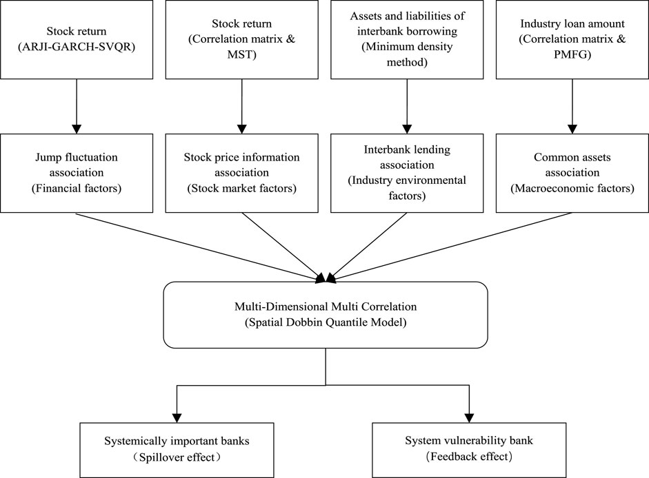
FIGURE 1. MDMC contagion of bank risk.

3 The Method of Multi-Dimensional Multi-Correlation Network Construction and Risk Contagion Measurement

3.1 Construction Method of Bank Risk-Related Contagion Network

We comprehensively characterize the risk-related contagion among commercial banks in four dimensions: jump risk spillover correlation, internal-related banking system, role of the financial market, and role of the capital market. A jump risk spillover-related network is an extreme risk-associated network in which the market affects the bank’s yield. Under normal conditions, the stock price information network forms a continuous fluctuation-related network of bank returns. The two methods describe the relevance of returns from different dimensions.

3.1.1 Constructing Jump Fluctuation-Associated Network With ARJI-GARCH-SVQR

Owing to extreme financial events, bank share price jumps are common [29]. Under the influence of financial market mechanisms, such as herding, investor sentiment, industry sector linkage, and common factors, a jump in the stock price of any bank leads to a sharp jump and fluctuation in the stock price of other banks in the same industry. Therefore, we use the ARJI-GARCH model to predict annual jump fluctuations. SVQR estimates the relative incremental conditional VaR to measure jump risk spillover, and the jump fluctuation-associated network is constructed using the overflow threshold method.

3.1.1.1 ARJI-GARCH Model

The ARJI-GARCH model consists of the conditional mean equation, jump setting, and conditional variance equation. The conditional mean equation is as follows:

$R_t=\mu +{\displaystyle \sum _{i=1}^l{\varphi }_i{R}_{t-i}}+\sqrt{h_t}{z}_t+{\displaystyle \sum _{k=1}^{n_t}{Y}_{t,k}},(17)$

where $\sqrt{h_t}{z}_t$ represents the impact of general information on the yield, called the continuous fluctuation term; $z_t$ is independent and identically distributed in the standard normal distribution, that is, $z_t\sim NID\left(\mathrm{0,1}\right)$; ${\displaystyle \sum Y_{t,k}}$ represents the impact of jump behavior on $R_t$, which is called the jump fluctuation term; $n_t$ indicates the number of jumps in the yield series from period $t-1$ to period $t$; and $Y_{t,k}$ represents the jump amplitude, which follows the normal distribution, with mean ${\theta }_t$ and variance ${\delta }_t^2$, that is, $Y_{t,k}\sim N\left({\theta }_t,{\delta }_t^2\right)$ with ${\theta }_t$ and ${\delta }_t^2$ being constant.

The jumping behavior is a random event. The number of jumps $n_t$ is assumed to obey the Poisson distribution with intensity ${\lambda }_t$ $\left({\lambda }_t>0\right)$, and the probability density function is

$P\left(n_t=j|{\Phi }_{t-1}\right)=\frac{e^{-{\lambda }_i}{\lambda }_t^j}{j!},j=\mathrm{0,1,2},\cdot \cdot \cdot ,(18)$

where ${\Phi }_t=\left[R_t,\cdot \cdot \cdot ,R_1\right]$ is the time t information set.

The expectation and deviation of conditional jump strength are

${\lambda }_t\equiv E\left[n_t|{\Phi }_{t-1}\right],(19)$

${\xi }_{t-i}\equiv E\left[n_{t-i}|{\Phi }_{t-i}\right]-{\lambda }_{t-i}={\displaystyle \sum _{j=0}^{\infty }jP\left(n_{t-i}=j|{\Phi }_{t-i}\right)}-{\lambda }_{t-i}.(20)$

If ${\lambda }_t=\lambda$ (constant), the ARJI-GARCH model degenerates into the CJ-GARCH model.

The conditional variance equation is composed of the lag term of the disturbance term and the lag term of the conditional variance,

$h_t=\omega +{\displaystyle \sum _{i=1}^q{\alpha }_i{\epsilon }_{t-i}^2}+{\displaystyle \sum _{i=1}^p{\beta }_i{h}_{t-i}}.(21)$

3.1.1.2 SVQR Model

The VaR refers to the maximum loss faced by financial assets under a certain probability level and within a specific holding period. It is implicitly defined as the q quantile, i.e.,

$\mathrm{Pr}\left(R^i\le Va{R}_{\tau }^i\right)=q,(22)$

where $R^i$ is the variable of bank $i$ for which the $Va{R}_{\tau }^i$ is defined.

The expression of the SVQR model by Takeuchi [30] is

$Y_t=f\left(X_t\right)={\mathbf{w}}_{\tau }^{\prime }\phi \left(X_t\right)+b_{\tau }+{\epsilon }_t,(23)$

where ${\mathbf{w}}_{\tau }$ represents the parameter vector, $b_{\tau }$ represents the threshold, ${\epsilon }_t$ is the disturbance term, and $\phi (\cdot )$ represents nonlinear mapping. The low-dimensional nonlinear function is transformed into a high-dimensional linear function, and the optimal parameters $\left(w,b\right)$ are obtained by training the sample set $\left\{Y_t;X_t\right\}$. The VaR estimated by the SVQR model is

$Va{R}_{\tau ,t}={\widehat{Q}}_{Y_t}\left(\tau |X_t\right)={\widehat{\mathbf{w}}}_{\tau }^{\prime }\phi \left(X_t\right)+{\widehat{b}}_{\tau }.(24)$

In this paper, the input variables of the SVQR model still refer to the research idea of the QR-GARCH model proposed by Taylor [31]. The jump volatility estimated by the ARJI-GARCH model is used for quantile regression to estimate jump VaR.

Conditional VaR is the mainstream index to measure the systemic financial risk contagion, and it is a conditional quantile. We use the method proposed by Adrian and Brunnermeier [32] to calculate Covar.

3.1.2 Using the Minimum Density Method to Build the Interbank Lending Network

Mutual lending between banks satisfies short-term liquidity needs. However, the interbank business usually has the problems of term and amount mismatch. The fund lender bears the credit risk of the fund user, which makes it easy to produce a cross-risk contagion caused by counterparty default. Most scholars use the maximum entropy method to estimate the lending network between institutions [33], which assumes that the associated network is completely connected. However, considering transaction and management costs, banks do not have a lending relationship with each institution in the system [34], and the relationship between the degree of risk contagion and interbank lending is not monotonic, showing the characteristics of stability and fragility [13,35]. Therefore, the indirect inference associated with the network’s MDM can be used [24,36]. The most effective sparse matrix is obtained by reducing the transaction costs in the lending relationship as much as possible. Therefore, we use bilateral exposure data and the MDM to construct the interbank lending-associated network.

The objective function of the minimum density method is

$\begin{array}{cc}\underset{x_{ij}}{\min }& c{\displaystyle \sum _{i=1}^n{\displaystyle \sum _{j=1}^{n}I\left(x_{ij}>0\right)}}\end{array},(25)$

where $c$ is the fixed cost required for interbank borrowing on behalf of the bank. For the illustrative function $I\left(x_{ij}>0\right)$, the following conditions are satisfied:

$I\left(x_{ij}>0\right)=\{\begin{array}{cc}1,& x_{ij}>0,\\ 0,& x_{ij}=0.\end{array}(26)$

The constraints are

$\{\begin{array}{l}{a}_i={\displaystyle \sum _{j=1}^n{x}_{ij}},\\ l_j={\displaystyle \sum _{i=1}^n{x}_{ij}},\\ x_{ij}\ge 0,\\ x_{ii}=0.\end{array}(27)$

The MDM is a matrix method. Each year’s interbank lending-associated network is solved, and the matrix elements represent the path weights between the two nodes. Therefore, a directed weighted network matrix is obtained.

3.1.3 Using the Minimum Spanning Tree Algorithm to Construct the Stock Price-Associated Network

Stock price information-related contagion is one of the main ways to drive fluctuations in investment returns in financial markets. This is an important source of systemic risk [37]. According to the degree of openness, financial market information is divided into historical, public, private, and new information. Financial market effectiveness theory and news theory and their empirical results show that the fully effective financial market price reflects all historical and public information rather than using high-value private information and new information in a fully effective market. New information advantage investments can obtain excess returns. Therefore, through the exchange and disclosure of private information, the disclosure and acquisition of new information, and the strong connection of information-associated networks, the two parties continue to share information, complex information mining, interpretation, and rapid transmission, forming stock price information infection. Therefore, in this study, the stock price information association takes institutions as nodes and the related coefficient of institutional stock return as an edge to construct the association relationship, measure the information association fluctuation, and adopt the minimum spanning tree algorithm (MST) [38] to build a stock price-associated network.

The calculation expression of the Pearson correlation coefficient is

${\rho }_{ij}^P=\frac{E\left(R_{it}{R}_{jt}\right)-E\left(R_{it}\right)E\left(R_{jt}\right)}{\sqrt{E\left(R_{it}^2\right)-E{\left(R_{it}\right)}^2}\sqrt{E\left(R_{jt}^2\right)-E{\left(R_{jt}\right)}^2}},(28)$

where ${\rho }_{ij}^P\in \left[-\mathrm{1,1}\right]$ is the Pearson correlation coefficient, $R_{it}$ represents the rate of return of the bank in the period, and $E\left(x_i\right)=\frac{1}{N}{\displaystyle \sum _{i=1}^N{x}_i}$ represents the desired function.

The higher the correlation of the return rate, the closer the relationship between the two banks in the network. The correlation coefficient matrix is transformed into a distance matrix, and the calculation formula is as follows:

$D_{ij}=\sqrt{2\left(1-{\rho }_{ij}\right)}.(29)$

The association relationship in the network is obtained through the MST algorithm using the distance matrix, and the Pearson correlation coefficient is used as the weight to obtain the bidirectional weighted associated network.

The specific steps are as follows. First, we arrange the distance matrix data in ascending order and select the two important nodes with the shortest distances to connect. Second, we choose the smallest important nodes in the remaining distance to continue the connection, and the spanning tree cannot form a closed-loop structure in the process. Third, we repeat this process until the number of connected edges is 1 less than the number of nodes and form a connected graph.

The commonly used methods are the Kruskal and Prim algorithms. We use the Kruskal algorithm to obtain a two-way weighted associated network composed of important nodes and paths.

3.1.4 Constructing the Value-Associated Network of Common Assets by Using the Plane Maximum Filter Graph Algorithm

According to the optimal portfolio theory, credit asset risk is decentralized. Banks’ assets are distributed across several industries. The development status and trends of the industry determine the quality of banks’ assets and liabilities. Thus, many banks with similar risk preferences will invest some of their credit assets in the same industry to hold common assets. The operational status jointly determines the value and risk of the common assets of these banks, profitability and value appreciation of these entity industries, and the changes in asset prices in the entity industries, forming the value of assets in the entity industries, and price and liquidity change as a link to the common linkage of the risk contagion network. Therefore, based on Cacioli et al. [6] and Fang and Zheng [26], we use the Kendall rank correlation coefficient to measure relevant asset value changes and the plane maximum filter graph algorithm to construct the associated network of holding common assets.

The proportion of assets invested by the bank in each industry is recorded as $\left\{x_{i1},x_{i2},\cdot \cdot \cdot ,x_{im}\right\}$. The weighted average value of the price index of each industry $\left\{p_1,p_2,\cdot \cdot \cdot ,p_m\right\}$ is used to represent the characteristic price of the bank,

$p_{it}^{\ast }=x_{i1}{p}_1+x_{i2}{p}_2+\cdot \cdot \cdot +x_{im}{p}_m.(30)$

The calculation formula of the bank’s logarithmic characteristic rate of return series $r_{it}$ is

$r_{it}=\ln \left(p_{it}^{\ast }/p_{it-1}^{\ast }\right),$

where $p_{kt}$ represents the price index of $k$ the industry at $t$.

We use the Kendall rank correlation coefficient to describe the consistency of changes in characteristic returns among banks,

${\rho }_{ij}^K=Prob\left[\left(r_{it}-r_{it-1}\right)\left(r_{jt}-r_{jt-1}\right)>0\right]-Prob\left[\left(r_{it}-r_{it-1}\right)\left(r_{jt}-r_{jt-1}\right)<0\right],(31)$

where ${\rho }_{ij}^K\in \left[-\mathrm{1,1}\right]$ is the Kendall rank correlation coefficient, $Prob\left[\left(r_{it}-r_{it-1}\right)\left(r_{jt}-r_{jt-1}\right)>0\right]$ represents the probability that the change in direction of the expected returns of the two banks is the same, and $Prob\left[\left(r_{it}-r_{it-1}\right)\left(r_{jt}-r_{jt-1}\right)<0\right]$ describes the probability that the expected returns of the two banks change in opposite directions.

The Kendall rank correlation coefficient matrix of the characteristic rate of return between banks is constructed to obtain a complete correlation network. As each bank will not lend to all industries, it will not associate with all banks because of lending in the same industry. The plane maximum filtered graph (PMFG) algorithm screens the network path to obtain the final industry-common loan-associated network.

The specific steps of the PMFG algorithm are as follows. First, we arrange the distance matrix weights of each effective path in ascending order, and only the node positions are reserved in the network. Second, we remove the paths in sequence and add them to the network to ensure that the paths added in each step maintain the plane graphic structure. Third, a network is formed when the total number of added paths is reached. Based on these steps, we can build a two-way industry-associated network with rights each year.

3.2 Integration Method of Multi-Industry-Related Infectious Networks

The bank risk-related contagion is complex, diverse, and intertwined, forming the superposition effect of risk contagions. Single-channel estimation seriously underestimates the systemic risk. We use addition to integrate four networks—jump fluctuation-associated network, interbank lending network, stock price information-associated network, and value correlation of common assets—to construct a four-tier interbank correlation contagion network.

The four risk-related network matrices are recorded as ${\mathbf{W}}^1={\left(a_{ij}^1\right)}_{n\times n}$, ${\mathbf{W}}^2={\left(a_{ij}^2\right)}_{n\times n}$, ${\mathbf{W}}^3={\left(a_{ij}^3\right)}_{n\times n}$, and ${\mathbf{W}}^4={\left(a_{ij}^4\right)}_{n\times n}$. First, the elements in each associated network matrix are row standardized to obtain the standardized matrix. Second, the elements at the corresponding positions of each matrix are added as elements in the multi-industry-associated network matrix. Finally, according to the cumulative superposition effect of risk contagions, a single associated network is combined into the MDMC network as follows:

$w_{ij}={\displaystyle \sum _{k=1}^4\left(a_{ij}^k/{\displaystyle \sum _{j=1}^n{a}_{ij}^k}\right)}=\frac{a_{ij}^1}{{\displaystyle \sum _{j=1}^n{a}_{ij}^1}}+\frac{a_{ij}^2}{{\displaystyle \sum _{j=1}^n{a}_{ij}^2}}+\frac{a_{ij}^3}{{\displaystyle \sum _{j=1}^n{a}_{ij}^3}}+\frac{a_{ij}^4}{{\displaystyle \sum _{j=1}^n{a}_{ij}^4}}.(32)$

3.3 Model Setting and Variable Description of Bank Comprehensive VaR Estimation in Multi-Dimensional Multi-Correlation

3.3.1 Model Setting

To verify the hypotheses obtained from the theoretical model analysis, we need to build a model that includes multi-dimensional factor-related, industry-related, and MDMC items simultaneously. General nonspatial models can only describe multi-dimensional factors, not multiple industry associations, and multi-dimensional factor correlations in multiple industry associations. Therefore, it cannot be used to verify these two assumptions. The general spatial econometric model can include the spatial correlation of the explained variable, spatial correlation of the explanatory variable, and spatial correlation of the error term at the same time. SDM is a general spatial econometric model, simultaneously including dependent variable spatially related items, independent variable items, and independent variable spatially related items.

Thus, we can measure the individual risk of banks determined by their factors and consider the contagion risk of MDMC network overflows between different bank risks and the contagion risk affected by the risk factors of connected banks. Therefore, we use a spatial weight matrix to reflect multiple industry associations. Taking bank yield as the explanatory variable, we use SDM to verify the four hypotheses. We add nonspatial terms of multi-dimensional factors to the model. If the parameters of these non-spatially related factors are significant, the hypothesis that the relevant factors have an important explanatory effect on bank risk is tenable. The spatial correlation terms of the multi-dimensional factors are added to the model. If these spatially related factors are significant, the hypothesis of multi-dimensional factor correlation is tenable. The spatial correlation term of the explained variable is introduced into the verification model. If the spatial correlation parameters of the explained variable are significant, the hypothesis of multiple horizontal correlations is tenable. If hypotheses 2 and 3 are true simultaneously, hypothesis 4 of the MDMC infectious network is true.

The matrix expression of SDM is

${\mathbf{Y}}_{\tau }={\rho }_{\tau }\mathbf{W}{\mathbf{Y}}_{\tau }+{\alpha }_{\tau }{\mathbf{\iota }}_n+{\mathbf{X}}_{\tau }{\mathbf{\beta }}_{\tau }+\mathbf{W}{\mathbf{X}}_{\tau }{\mathbf{\theta }}_{\tau }+\mathbf{\epsilon },(33)$

where $\mathbf{Y}$ is the logarithmic yield vector of bank, $\tau$ is the significant level of quantile-estimated VaR, $\rho$ is the spatial autoregressive correlation coefficient, $\mathbf{W}={\left(w_{ij}\right)}_{n\times n}$ is the spatial weight matrix, and $\mathbf{\alpha }$ is the vector of intercept term. The diagonal elements of the ${\mathbf{\iota }}_n$ matrix are 1, and the other elements are 0. $\mathbf{X}$ is the explanatory variable vector. $\mathbf{\beta }$ and $\mathbf{\theta }$ are the coefficient matrix of each explanatory variable and the explanatory variable’s spatial lag term.

In the financial stock market, the impact of upward and downward risk spillover effects is different. The extreme returns of the left and right tail have other state characteristics. We use the standard deviation as the threshold to divide the bank yield series into three regions with normal fluctuation characteristics, namely, positive shock, negative shock, and wave, which represent the three characteristic states of high-value shock, medium-value shock, and low-value shock, respectively,

$R=\{\begin{array}{cc}{R}^P,& R\in \left(\sigma ,\infty \right),\\ R^W,& R\in \left[-\sigma ,\sigma \right],\\ R^N,& R\in \left(-\infty ,-\sigma \right).\end{array}(34)$

The direct, indirect, and total effects of spatial correlation can be obtained through the decomposition and summary calculation of the spatial correlation terms [39].

We construct an SDM and use the quantile estimation method to verify the research hypothesis, estimate banks’ conditional VaR, and decompose the systemic financial risk contagion effect.

3.3.2 Variable Selection

According to the theoretical analysis results of the second part, bank risk factors are multi-dimensional, mainly including the bank’s assets and liabilities, financial factors, bank stock market factors, industry-related environmental factors, and macroeconomic factors. To verify hypothesis 1 (multi-dimensional risk factors) and hypothesis 2 (multi-dimensional factor-related infection) proposed in Section 2, we select the factor indicators of these four dimensions as the model’s explanatory variables.

3.3.2.1 Bank Financial Factors

We use the non-performing loan ratio to measure the quality of bank credit assets [40]. The return on total assets reflects the bank’s operating performance [41]. The deposit loan ratio measures the matching degree of bank liquidity [42].

3.3.2.2 Bank Stock Market Factors

We use the conditional volatility calculated by the jump-GARCH model to reflect the risk of bank stock price fluctuation. The turnover rate is used to reflect the activity of bank stock trading, purchase intention, and liquidity. Combined with the optimism and pessimism reflected by the rise and fall in stock prices, we measure investor sentiment toward bank stocks [43]. The Herfindahl index in the banking industry reflects the concentration of bank lending risk [44]. The log return and volatility of the Shanghai composite index are selected to reflect the overall value level and change risk of the bank stock market [45].

3.3.2.3 Banking Business Environment Factors

The short-term liquidity spread is measured by the difference between the 6-month Shibor interest rate and the 6-month treasury bond spot yield, reflecting the risk of liquidity shortage in the banking industry. Using the change of 6-month treasury bond interest rate to measure the change in the short-term treasury bond yield reflects the interest rate risk of liquidity financing [46]. The difference between the spot yields of 10-year corporate bonds and 10-year treasury bonds is selected to reflect the change in enterprise credit spread in the real economy [47].

3.3.2.4 Macroeconomic Factors

We select the CPI to reflect the price level [48]. The GDP growth rate is selected to reflect the speed of economic development [49]. China’s real estate boom index is selected to reflect the national real estate industry [50].

The specific variable indicators, characterization variables, interpretation, and calculation methods are summarized in Table 1.

TABLE 1

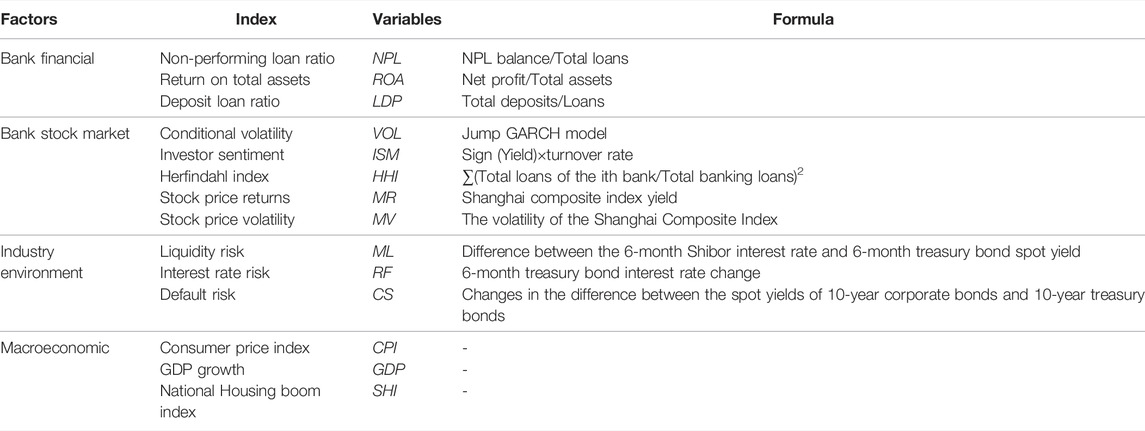
TABLE 1. Multi-dimensional factor variables of bank risk estimation.

4 Estimation Results and Analysis of Banking Systemic Risk in the Framework of Multi-Dimensional Multi-Correlation Contagion

We select 14 commercial banks listed before 2008, including 4 state-owned banks, namely, the Bank of Communications (BCM), Industrial and Commercial Bank of China (ICBC), China Construction Bank (CCB), and Bank of China (BOC); 7 joint-stock banks, namely, Ping An Bank (PAB), Shanghai Pudong Development Bank (SPDB), Huaxia Bank Co., Ltd. (HXBC), China Minsheng Banking Corp., Ltd. (CMBC), China Merchants Bank Co., Ltd. (CMB), China Industrial Bank Co., Ltd. (CIB), and China CITIC Bank (CITIC); and 3 other urban development banks, namely, Bank of Ningbo (BON), Bank of Nanjing Co., Ltd. (BNC), and Bank of Beijing (BOB). The total assets of 14 commercial banks account for approximately 80% of the total assets of China’s banking industry, accounting for 85% of the number of banks recognized by regulatory authorities as systemically important banks. Therefore, the number of commercial bankers we selected is sufficiently representative. Due to data availability, the period is selected as the weekly data from 2007 to 2019. The original daily data are transformed into weekly data, and the corresponding weekly data are directly selected. The quarterly macro-data are obtained by cubic spline interpolation, and the original data of all indicators are obtained from the Wind database. Descriptive information on the bank yield data is shown in Table 2.

TABLE 2

TABLE 2. Descriptive statistics and characteristic test of the yield.

4.1 Characteristic Description of Multi-Dimensional Multi-Correlation Network

4.1.1 Characteristic Description of Jump Risk Spillover Correlation Network

We use the ARJI-JUMP-SVQR model to calculate the conditional VaR, including jump fluctuation, and then use the overflow threshold method to construct the directed weighted jump fluctuation risk overflow network incidence matrix. The annual average network topology relationship is shown in Figure 2, and the first layer is shown in Figure 4.

FIGURE 2

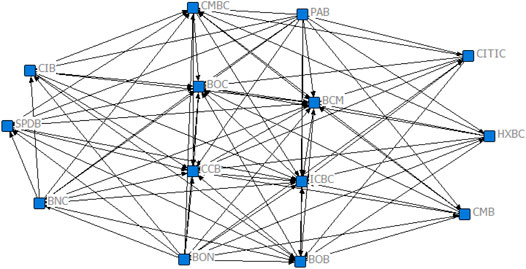
FIGURE 2. Jump risk correlation network of commercial banks.

Figure 2 shows that the network matrix contains both single- and two-way overflows. Individual banks act as risk spillovers and risk absorbers, reflecting the complexity of risk correlation networks. Large state-owned banks, such as the ICBC, BOC, CCB, and BCM, are located in the center of the network. Joint stock banks such as PAB, CMBC, and CIB are located at the edge of the network. State-owned banks have strong relevance and risk contagion at the core.

We draw a network association diagram every 4 years, as shown in Figure 3.

FIGURE 3

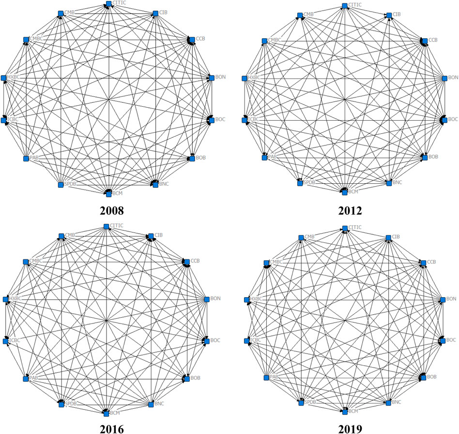
FIGURE 3. Jump risk network of commercial banks.

Figure 3 shows that the network relevance of each year is high. Some nodes are only connected with a few nodes, but some key nodes are connected with a considerable number of nodes (e.g., large state-owned bank nodes), which indicates that the associated network has the characteristics of scale-free. The banking system has the characteristics of robust and fragile, and the possibility of infectious default is low. However, if extreme risk events impact some high correlation nodes, they will be quickly transmitted to other related banks through network correlation, resulting in serious damage to the whole financial system.

4.1.2 Description and Analysis of the Characteristics of the Interbank Lending-Related Network

The annual interbank lending network data using the MDM are shown in Table 3. Figure 4 shows the interbank lending network diagram of the second layer.

TABLE 3

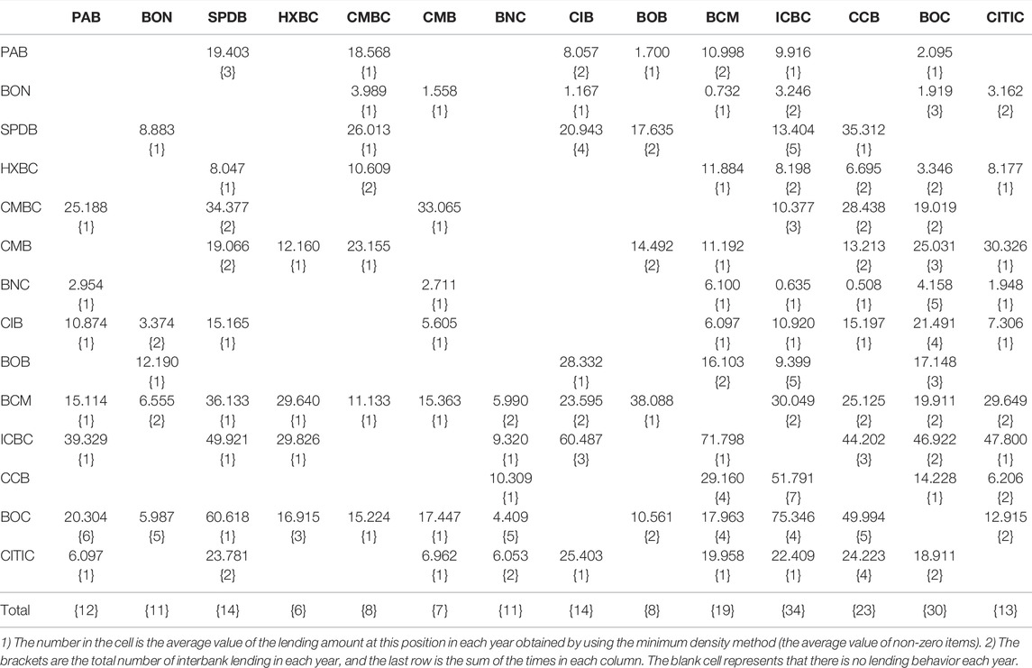
TABLE 3. Statistics of interbank lending networks from 2008 to 2018.

FIGURE 4

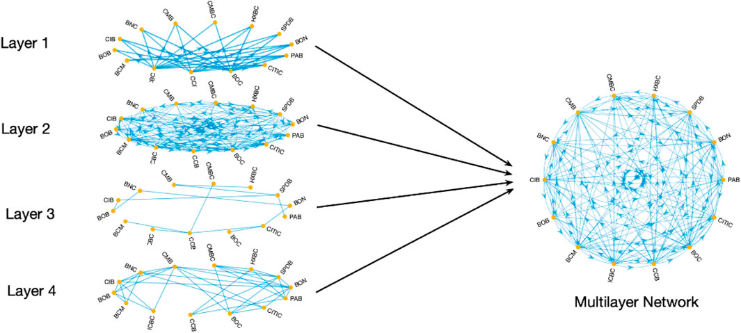
FIGURE 4. Four layers of the risk correlation network.

As shown in the second-layer diagram in Table 3 and Figure 4, the lending behavior of large state-owned banks involves a large range of banks and a large number of times, which indicates that asset liquidity is strong and accompanied by high liquidity risk. When holding many small bank assets, the occurrence of extreme risks will lead to a wide range of risk spillover and infectious events.

4.1.3 Description and Analysis of the Characteristics of Bank Stock Price-Associated Network

The Pearson correlation coefficient of continuous fluctuation is used to measure the correlation of stock price information. The MST algorithm is used to construct the associated network of stock price information. The undirected weighted stock price information-associated network matrix is obtained, as shown in Table 4. A diagram is drawn to obtain the layer three network diagram shown in Figure 4.

TABLE 4

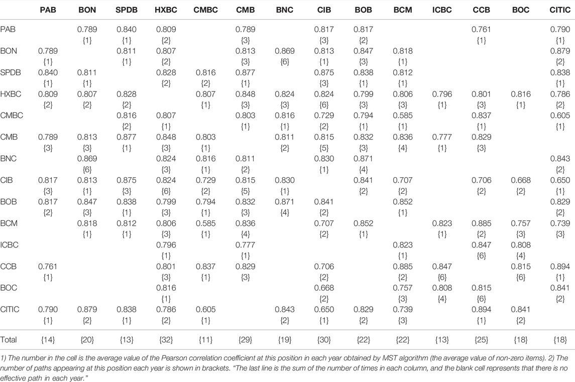
TABLE 4. Statistics of stock price-related networks of banks from 2008 to 2018.

According to the third-layer network diagram in Table 4 and Figure 4, HXBC, CIB, CMB, and CCB are often located on the core path. All banks’ cumulative number of connections exceeds 11, meaning that there will be connections with at least one bank every year, with a wide range of connections. The correlation coefficient on the effective node is roughly between 0.6 and 0.9, and the overall correlation is obvious.

4.1.4 Characteristic Description and Analysis of the Associated Network of Holding Common Assets

First, we select the loan balance of each banking industry in 16 industries from the end of 2008 to the end of 2018 and calculate the loan proportion of each industry of each commercial bank as the characteristic price weight. The top five industries in terms of the proportion of loans are manufacturing, real estate, transportation, wholesale and retail, and business services. We select the price indexes of various industries from 2008 to 2018, calculate the weighted average value, obtain the characteristic price of common assets held by commercial banks, and obtain the characteristic logarithmic rate of return. Finally, the Kendall rank correlation coefficient between characteristic log returns is calculated to measure the relevant changes in the asset value. The PMFG algorithm is used to construct the associated network of holding common assets, and the results are listed in Table 5. A diagram is drawn to obtain the associated network diagram of common assets held by the bank, as shown in the fourth layer diagram in Figure 4.

TABLE 5

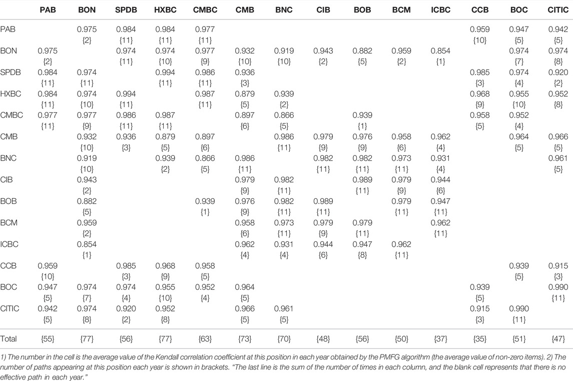
TABLE 5. Statistics of related networks in various banking industries from 2008 to 2018.

Table 5 and the fourth layer diagram in Figure 4 show that the number of connections of large state-owned banks such as ICBC and CCB is low, which indicates that their characteristic rate of return is not affected by market fluctuations and the situation is relatively stable. Joint-stock banks such as HXBC and CMB and urban development banks such as BON and BNC have many network connections, which shows that these banks’ characteristic rate of return evidently follows market changes and is vulnerable to fluctuations.

4.1.5 Feature Description and Analysis of Multi-Dimensional Multi-Correlation Networks

The four aforementioned bank risk correlation networks are superimposed. After calculating the average value of network node connections at each layer annually and screening the paths, a four-layer risk correlation network is formed. Then, according to Eq. 1, the weighted average is integrated into a four-layer directed weighted correlation network. The multilayer network is formed by the superposition of the jump-risk overflow network layer (layer 1), interbank lending-related network layer (layer 2), the bank stock price-related network layer (layer 3), and a common asset-related network layer (layer 4). The jump risk spillover and interbank lending-related layers are directed toward the weighted related network layers. The related bank stock prices and holding common assets are undirected related network layers. The results are shown in the multiple network diagram in Figure 4.

The average characteristic indexes of the nodes in each layer network and multilayer network are listed in Table 6.

TABLE 6

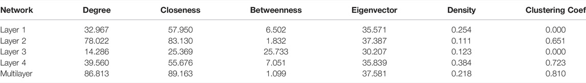
TABLE 6. Characteristic description of multilayer networks.

Table 6 shows that the MDMC network superimposes risk contagion effects in all directions and forms almost a fully connected network between bank nodes. Therefore, it has the highest degree of centrality and closeness centrality and reduces each bank’s betweenness centrality to 1.099%. Compared with the associated network for each layer. The MDMC network has a high feature vector centrality and clustering coefficient, which shows that after superposition, the connectivity between nodes is higher, and the centrality of nodes as a whole is higher, reflecting the universality and complexity of risk infection.

The MDMC network comprehensively considers the multi-channel characteristics of risk contagion and reasonably explains the possibility of changing overflow channels at nodes. High connectivity also better explains the feedback effect of risk in the contagion process, which is more in line with the characteristics of extreme risk transmission. Therefore, the time-varying MDMC network constructed by year describes the risk-contagion process. The characteristics of time-varying MDMC networks are listed in Table 7.

TABLE 7

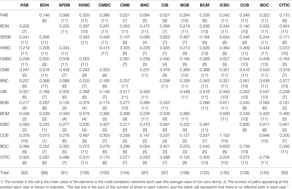
TABLE 7. Statistics of characteristics of time-varying MDMC networks from 2008 to 2018.

4.2 Results and Analysis of Comprehensive VaR Estimation of Banks Under Multi-Dimensional Multi-Correlation Networks

4.2.1 Descriptive Statistics

Table 8 shows the statistical characteristics of the weekly data description of the multiple jump VaR estimation indicators.

TABLE 8

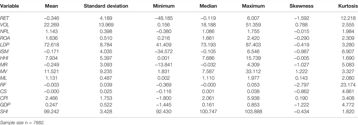
TABLE 8. Description and statistics of variable data.

The financial and macro-indicators in Table 8 are quarterly data. We use cubic spline interpolation to convert the quarterly data into weekly data, and the rest are converted through calculation or directly selected weekly data. The mean and variance of each index are within a reasonable range, and the return series and a small number of explanatory variables deviate from the normal distribution. Quantile regression can be used for robust and effective estimation.

4.2.2 Spatial Correlation Analysis and Model Identification Verification

The Moran index reflecting the degree of spatial correlation in all observations is significantly greater than zero, indicating a significant positive spatial correlation in the bank return series under the action of the MDMC network. The LM lag and LM error tests reject the original hypothesis, indicating interaction effects between the model’s explanatory variables and error terms. Robust LM error and LM lag tests also prove the rationality of the spatial lag relationship and spatial error correlation. The Wald a posteriori test shows that the SDM with a nested structure is more suitable for this study. These statistical test results show that hypotheses 2 and 3 proposed in the theoretical analysis are significantly valid. Therefore, we consider using the quantile estimation method of the SDM to estimate and analyze the VaR.

4.2.3 Estimation Results and Analysis of Spatial Dubin Panel Quantile Regression of Bank Comprehensive Financial Risk

First, the SDQR is conducted for the return series of the entire sample period. Then, the bank return series is divided into three regions with the standard deviation as the threshold, that is, the positive impact with an increase of more than one standard deviation, the negative impact with a decrease of more than one standard deviation, and the volatility within a positive and negative standard deviation. The SDQR is estimated for the three regions, and the results are listed in Table 9.

TABLE 9

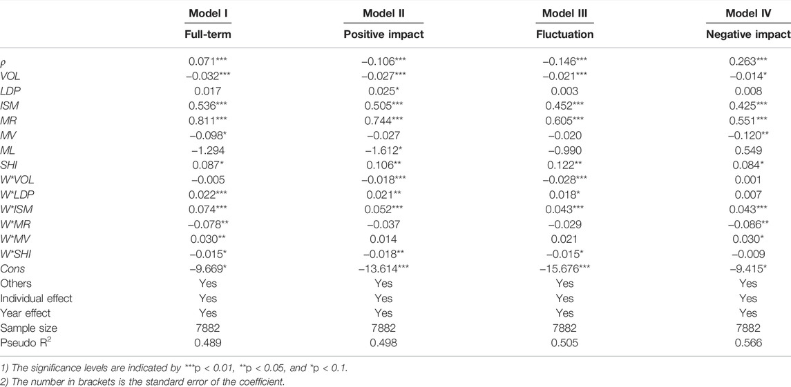
TABLE 9. Results of SDQR under the MDMC network.

As seen in Table 9, the spatial autoregressive correlation coefficient of the model in each stage is positively significant, which indicates that the four-channel contagions of jump spillover correlation, interbank lending correlation, and stock price information correlation, and holding common assets correlation are significant. The cumulative superposition effect of four-channel contagion is also significant. The change in the return rate of affiliated banks in a time-varying spatial multilayer network will have a significant positive impact on the VaR of target banks. Extreme risk events in affiliated banks are likely to overflow risk to the target bank through MDMC networks, resulting in local and systemic risks. Measuring the bank risk contagion requires an all-around integration of the important contagion effects. The single- and double-path contagion of banking systemic financial risk underestimates the contagion effect. This conclusion also provides a theoretical basis for the simulation and calculation of risk contagion evolution, which shows that hypothesis 3 proposed in Section 3 is significantly valid. The four bank risk-related infectious networks interact, forming multiple interbank-related contagious networks.

We use the SDQR to estimate the VaR of banks. As an explanatory variable, the risk factor parameter is significant, indicating that it includes the individual risk caused by risk factors. Spatial autocorrelation is significant, showing that different bank risks are transmitted through four paths. Five parameters in the spatial correlation terms of the six explanatory variables are significant, including the individual risk caused by the risk factors and the spillover risk caused by the risk factors of related banks. Therefore, the VaR estimated by the SDQR in this study is the bank’s comprehensive risk, including individual risk and two infectious risks. The simulation analysis literature cannot monitor the comprehensive risk degree of banks but can only provide simulation evolution results, which is not suitable for systematic financial risk monitoring. Therefore, we compensate for the deficiency of the existing research literature on risk contagion simulation calculation and provide a methodological basis for the entire process visualization of risk contagion path simulation.

From the results for the entire period, the conditional volatility of the bank has a significant direct negative effect on the VaR of the target bank. Investor sentiment, stock price returns, stock price volatility, and the national housing boom index have a significant direct positive impact on the VaR of the target bank. The deposit loan ratio of affiliated banks and market investor sentiment also affect the risk of affiliated banks, which has a significantly positive spillover effect on the risk of target banks. The market share price return and national housing boom index have a significant negative spillover effect on the target bank risk by affecting the related bank risk.

From the results of the zoning system, the conditional volatility of banks has a significant negative direct impact in the three zoning systems. Investor sentiment, stock price returns, and the national housing boom index have a significant positive direct impact. Investor sentiment also has a significant positive spillover effect on related bank risk. In addition, banks’ conditional volatility has a significant positive effect on the positive shock and shock fluctuation regime. The conditional volatility of affiliated banks also has a significant negative spillover effect. The deposit loan ratio of affiliated banks has a significant positive spillover effect. The national housing boom index has a significant negative spillover effect on the risk of target banks by affecting the risk of related banks. The deposit-to-loan ratio positively impacts bank liquidity and directly impacts bank liquidity risk. In the negative impact zone system, the market share price volatility has a significant negative direct impact on the risk of target banks.

The market stock price return has a significant negative spillover effect on the target bank risk by affecting the related bank risk, while the market stock price volatility has a significant positive spillover effect on the target bank risk by affecting the related bank risk. The significance of the estimated values of these parameters shows that hypotheses 1 and 2 proposed in the theoretical analysis part are significantly valid. Bank risk factors are both multi-dimensional and interactive. Hypotheses 2 and 3 are significantly valid in the unified verification framework, confirming that hypothesis 4 is valid. A multi factor-related contagion and a multi-industry-related contagion exist significantly at the same time and interact to form a MDMC contagion network.

By comparing the results of the whole period and different zoning systems, it can be seen that the symbols of the parameters of the risk factors and their spatial correlation items are the same, but the estimated values are quite different, which indicates that there is a jump impact on different market risks. The direct and spillover feedback effects of the risk factors are asymmetric, and the response to positive shocks is large.

5 Identification Results and Analysis of System Importance in Multi-Dimensional Multi-Correlation Networks

To understand the characteristics of MDMC networks further, we use the conclusions obtained from the above model verification to decompose the spillover contagion effect of bank risk and identify systemically important factors, systemically important banks, and systemically vulnerable banks.

5.1 Decomposition Method of Bank Risk Spillover Contagion Effect in Multi-Dimensional Multi-Correlation Networks

We use the LeSage and Pace [51] method to decompose the spatial econometric model. The partial differential of the SDM shown in Eq. 31 can be obtained, and the quantile partial effect matrix of the explained variable Y to the explanatory variable X is

$\begin{array}{l}{\mathbf{S}}_k\left(\mathbf{W}\right)={\left(\mathbf{I}-\rho \mathbf{W}\right)}^{-1}\left(\mathbf{I}{\beta }_k+\mathbf{W}{\theta }_k\right)\\ ={\left(I-\rho \mathbf{W}\right)}^{-1}\left[\begin{array}{cccc}{\beta }_k& w_{12}{\theta }_k& \cdots & w_{1N}{\theta }_k\\ w_{21}{\theta }_k& {\beta }_k& \cdots & w_{2N}{\theta }_k\\ ⋮& ⋮& \ddots & ⋮\\ w_{N1}{\theta }_k& w_{N2}{\theta }_k& \cdots & {\beta }_k\end{array}\right]\end{array}.(35)$

The influence of the change in a specific independent variable of an organization on a dependent variable is the direct effect $\overline{\mathbf{M}}{\left(k\right)}_D$, which is numerically expressed as the mean of the diagonal elements of the matrix ${\mathbf{S}}_k\left(\mathbf{W}\right)$,

$\overline{\mathbf{M}}{\left(k\right)}_D=n^{-1}tr\left({\mathbf{S}}_k\left(\mathbf{W}\right)\right).(36)$

The impact of changes in the independent variables of institutions on the dependent variables of affiliated institutions is an indirect (spillover) effect $\overline{\mathbf{M}}{\left(k\right)}_I$, which is numerically expressed as the mean of the sum of the non-diagonal element columns of the matrix ${\mathbf{S}}_k\left(\mathbf{W}\right)$,

$\overline{\mathbf{M}}{\left(k\right)}_I=n^{-1}{\iota }_n^{\prime }{\mathbf{S}}_k\left(\mathbf{W}\right){\iota }_n-\overline{\mathbf{M}}{\left(k\right)}_D.(37)$

The sum of the direct and indirect effects caused by the change in an institution’s specific independent variables is the total effect $\overline{\mathbf{M}}{\left(k\right)}_T$, which is expressed as

$\overline{\mathbf{M}}{\left(k\right)}_T=\overline{\mathbf{M}}{\left(k\right)}_D+\overline{\mathbf{M}}{\left(k\right)}_I.(38)$

5.2 System Importance Analysis Method in Multi-Dimensional Multi-Correlation Network

The analysis in this section mainly identifies important factors, systemically important financial institutions, and systemically vulnerable financial institutions. Systemically important factors refer to those whose changes will have a significant negative impact on the risk status of financial institutions and the entire financial system. They directly impact financial institutions and infect the system through their risk overflow of financial institutions, resulting in systemic risks. According to the characteristics of systemically important factors, the total effect of risk factors, including the direct impact on institutional risk (direct effect) and indirect impact on financial system risk (indirect effect), can be used to identify. The total effect of the risk factors is calculated as Eq. 35.

Systemically important financial institutions refer to financial institutions with a large scale and wide range of connections, which will significantly impact-related institutions or the whole financial system in case of risk events. It has a large scale, obvious correlation and a high spillover effect (i.e., indirect effect). The total spillover effect $\mathbf{IE}$ of banks can be used to identify systemically important banks,

$\mathbf{I}{\mathbf{E}}_{\tau }={\alpha }_{\tau }{\mathbf{\iota }}_n+{\displaystyle \sum {\mathbf{X}}_{it}\overline{\mathbf{M}}{\left(k\right)}_{I,\tau }}.(39)$

Systemic vulnerability refers to financial institutions that are vulnerable to risk events and have a high degree of absorption correlation. They are vulnerable to the greater negative impact of the risk spillover contagion of related banks, and the feedback effect of their risk spillover. Under this effect, they can easily go bankrupt or face difficulties. The feedback effect $\overline{\mathbf{M}}{\left(k\right)}_F$ describes the feedback transmission effect of the spatial spillover effect among related institutions, including the cumulative effect of feedback transmission to the institution, recorded as ${\mathbf{R}}_k\left(\mathbf{W}\right)=\left[{\left(\mathbf{I}-\rho \mathbf{W}\right)}^{-1}-\mathbf{I}-\rho \mathbf{W}\right]\left(\mathbf{I}{\beta }_k+\mathbf{W}{\theta }_k\right)$. The feedback effect is numerically expressed as the column and mean of the matrix ${\mathbf{R}}_k\left(\mathbf{W}\right)$,

$\overline{\mathbf{M}}{\left(k\right)}_F=n^{-1}{\iota }_n^{\prime }{\mathbf{R}}_k\left(\mathbf{W}\right){\iota }_n.(40)$

Therefore, the total feedback effect $\mathbf{FE}$ of a bank can be calculated by decomposition, and the system vulnerability bank can be identified as follows:

$\mathbf{F}{\mathbf{E}}_{\tau }={\alpha }_{\tau }+{\displaystyle \sum {\mathbf{X}}_{it}\overline{\mathbf{M}}{\left(k\right)}_{F,\tau }}+{\mathbf{v}}_t.(41)$

5.3 Identification Results and Analysis of Systemic Importance Risk Factors From the Perspective of the Total Effect

The total effect of the risk factor variables reflects the effects of this factor on the VaR of all banks. The total effect of each factor can be calculated using Eq. 35, and the specific results are listed in Table 10.

TABLE 10

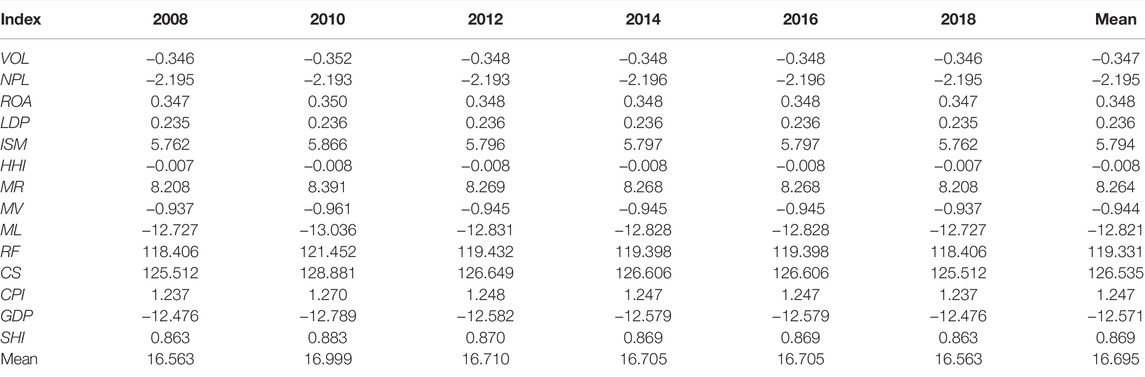
TABLE 10. Total effects of risk factors.

It can be seen from Table 10 that default risk, interest rate risk, liquidity risk, and the total effect of the GDP growth rate are the four most influential factors. The total effect of the factors includes the direct effect on the VaR of the explained institution and the multilayer spillover effect on the VaR of related institutions. The former forms the individual bank risk, the latter forms the bank contagion risk, and the sum of the two forms the comprehensive risk. The large effect of these factors shows that they play a significant role in the formation, outbreak, and spread of bank vulnerability and systemic financial risk. Therefore, these systemically important factors are the key operational objectives and indicators of micro-prudential supervision and macroprudential supervision and regulation. This conclusion enriches the literature on single- and dual-channel infections. The contagion simulation research literature mainly analyzes the sensitivity pressure of simulation algorithm parameters and identifies sensitive factors, such as the asset price sensitivity coefficient and interbank loan ratio [5]; Ccnnectivity, market density, lending ratio, and leverage ratio [52]; and price shock index and loss rate [2]. However, it is impossible to perform an ergodic scenario stress analysis of exogenous systemic risk factors.

5.4 Identification Results and Analysis of Systemically Important Institutions From the Perspective of Total Spillover Effect

The total effect of spatial spillover includes the direct effect of risk factors on the institution and the indirect effect of risk spillover on affiliated institutions. The total indirect effects of each institution in each year are calculated and ranked using Eq. 37. The results are presented in Table 11.

TABLE 11

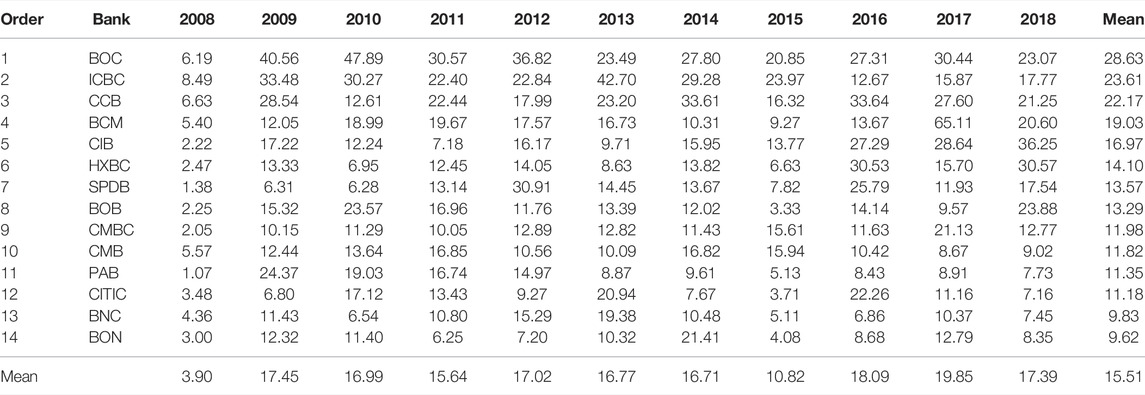
TABLE 11. Total spillover effects of banks.

It can be seen from the average annual total effect in Table 11 that the bank spillover risk was high in the following 3 years of the financial crisis and stock disaster in 2015. The overall spillover effect shows a decreasing annual trend, which shows that the degree of risk spillover is reduced annually, and systemic risk has been well controlled. BOC and ICBC are in the highest quartile range of the bank mean of the total effect. The total spillover effect of the four large state-owned banks is stable at the forefront of each year. They are large scale and highly related and should belong to systemically important institutions. Suppose that extreme risk events impact large state-owned banks. In this case, the risk will be transmitted to relevant institutions under the action of MDMC networks, which is likely to cause systemic risk and is the first tier of systemically important financial institutions.

The total spillover effects of the CIB and HXBC are in the third quartile range. The total effect of other banks is in the lowest quartile range. According to the results of the two-channel correlation contagion from asset and price, the ranking of systemic importance is considered to be based on the number of bank failures is ICBC, CCB, BOC, and the Agricultural Bank of China [2]. The main reason BOC surpasses ICBC under MDMC networks is that the number of effective paths associated with the BOC’s stock price information and holding common assets is greater than that of ICBC. The number of effective paths for the BOC’s jump association, the interbank lending association, the ICBC’s jump association, and the interbank lending association is 13, 30, 12, and 34, respectively. The number of quadruple association paths for BOC is 112, and the number of significant association paths for ICBC is 93.

5.5 Identification Results and Analysis of System Vulnerability Mechanism From the Perspective of Total Feedback Effect

The total feedback effect reflects the institution’s risk factors and extreme-risk events. After the negative impact infects affiliated institutions, it reacts to the institution, resulting in the secondary effect of the risk. The total feedback effect of each organization in each year is calculated using Eq. 38 and ranked. The results are shown in Table 12.

TABLE 12

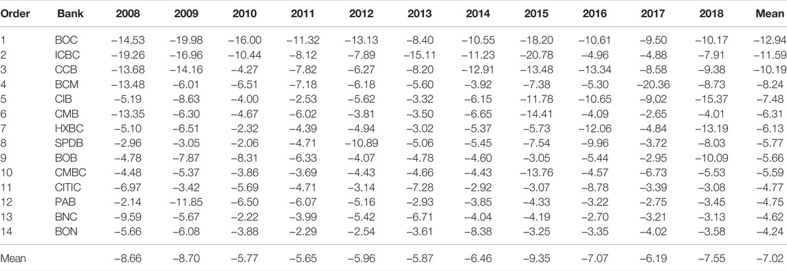
TABLE 12. Total feedback effect of banks.

It can be seen from Table 12 that the total feedback effect of the banking industry during the financial crisis in 2008 and the stock market disaster in 2015 is high and then shows a decreasing annual trend, which shows that under the action of crisis management measures, the feedback effect of risk spillover is declining annually. The acceleration momentum of the risk contagion is well controlled.

Large banks are still at the forefront of each year from the mean of banks, with a total feedback effect. BOC, ICBC, CCB, and BCM are among the top four banks with a total feedback effect, which shows that the total spillover effect and total feedback effect are also large. The four state-owned banks are the key nodes with high centrality in the four related networks. These are the contagion path of risk spillover and the feedback contagion path of risk spillover. Without considering the banks’ risk mitigation ability, the four state-owned banks have the characteristics of systemically important institutions and systemic vulnerability, which reflects the characteristics of “both the stability and vulnerability” of China’s financial institutions. This conclusion is similar to that of research on the dual-channel contagion [53]. The total feedback effect of the Industrial Bank, China Merchants Bank, and Huaxia Bank is large, and the total spillover and feedback effects of the Industrial Bank and Huaxia Bank are large, mainly due to the relatively large correlation paths of significant spillover and feedback absorption of the two banks. The total feedback effect of China Merchants Bank exceeds that of Shanghai Pudong Development Bank, which has a large total spillover effect. This is mainly because the number of significant paths of the China Merchants Bank’s MDMC networks is 104. The number of significant paths of Shanghai Pudong Development Bank’s MDMC network is 91, and its interbank lending correlation and jump correlation ratio are large.

6 Conclusion

The existing literature mainly uses the simulation experimental calculation method to study the evolution process of the bank risk double correlation contagion and performs parameter sensitivity analysis. The effectiveness of the results largely depends on the rationality of the parameter value selection and algorithm design, which can only describe the evolution mechanism of contagion diffusion and cannot accurately measure the effectiveness of risk infection. The existing literature rarely studies the problem of bank multi-channel contagion completely based on actual data. However, many studies have shown four correlation paths in the bank risk contagion mechanism. Multiple correlation paths coexist simultaneously, and the superposition effect produced by the interaction produces a stronger contagion destructive power. Therefore, this study integrates the contagion effects of four paths—jump correlation, interbank lending correlation, stock price information correlation, and holding common assets correlation—constructs a MDMC network matrix, and uses the quantile estimation of the spatial Dubin panel model to estimate the comprehensive risk value of banks, including individual risk and contagion risk. We decompose the spillover feedback contagion effect, summarize it according to factors, banks, and time, and analyze systemically important factors, systemically important financial institutions, and systemically vulnerable institutions.

The conclusions of this study are as follows. First, the cumulative superposition effect of the four channel-related infections is very significant. Second, the banks’ conditional volatility has a significant direct negative effect on the VaR of the target bank. Investor sentiment, stock price returns, stock price volatility, and the national housing boom index have a significant direct positive impact on the VaR of the target bank. The deposit loan ratio of affiliated banks and market investor sentiment also affect the risk of affiliated banks, which has a significant positive spillover effect on the risk of target banks. The market share price return and national housing boom index have a significant negative spillover effect on the target bank risk by affecting the related bank risk. The total effect of default risk, interest rate risk, and liquidity risk in industry factors and the GDP growth rate of macro-factors are the top four systemically important risk factors, followed by the change in stock price returns of market factors and investor sentiment. Third, the MDMC network of the four major state-owned banks is significantly higher than that of joint-stock banks and urban development banks. The four major state-owned banks have the characteristics of systemically important institutions and strong characteristics of system vulnerability. The total spillover effect of the CIB, HXBC, and SPDB is large, while the total feedback effect of the CIB, CMB, and HXBC is large.

Based on the aforementioned conclusions, we accurately prevent and control risks. First, we should design a market circuit breaker, market maker, and counter-cyclical dynamic adjustment of the margin ratio of credit financing transactions and other stock-market-related contagion suppression mechanisms. Improve the monitoring index system and information disclosure system for the interbank lending ratio and industry risk. We focus on the four paths of monitoring jump correlation, interbank lending correlation, stock price information correlation, and holding common assets correlation to resolve the superposition effect of MDMC network infections. Second, we focus on banks’ comprehensive risk, including individual and infectious risks. Build a counter-cyclical dynamic regulatory system to mitigate the common impact of macroeconomic factors, such as the GDP growth rate and the national housing boom index, on systemic financial risks. Finally, we set additional capital requirements for liquidity and residual risks. Then, we build the expected deficit (ES) model to improve attention to risk events with low frequency and high destructive power. We improve the supervision of additional capital of systemically important financial institutions. We refine the asset classification scheme to prevent regulatory arbitrage. We improve and optimize the exposure weight structure and credit conversion coefficient to improve risk sensitivity. We will optimize the implementation plan of the internal rating method and improve the microprudential supervision of financial institutions with systemic vulnerabilities.

In addition, our research focuses solely on the banking industry. We believe that the systemic importance of banks not only comes from their internal risks but also receives the extreme risk impact of other external banks, which has certain limitations. As an important part of the financial market, banking industry risk is not only caused by internal factors but also closely related to external industries and macroeconomic situations. Future research will further extend the linkage perspective of financial system risk, expand the industry network into the financial system network, investigate the extreme risk of banks again, and determine its systemic importance.

Data Availability Statement

The original contributions presented in the study are included in the article/supplementary material, further inquiries can be directed to the corresponding author.

Author Contributions

Conceptualization: ZW and QZ; study the literature, determine the research problems and objectives, and select the theme and methodology: ZW, QZ, and LQ; design the research content, method, and technical route and write the introduction and literature review software: ZW, QZ, and LQ; validation: QZ; formal analysis: ZW and QZ; investigation: ZW, QZ, and LQ; data curation and visualization: ZW and QZ; writing—original draft preparation: QZ; writing—review and editing: ZW, QZ, and LQ; supervision and project administration: ZW; funding acquisition: ZW and LQ. All authors have read and agreed to the published version of the manuscript.

Funding

This research was funded by the General project of NSFC: Research on multi-dimensional and multiple contagions of Banking Systemic Financial Risk in structural change, grant number (71973098) and Youth project of NSFC: Financial risk early-warning based on high dimensional supervised network (12105178).

Conflict of Interest

The authors declare that the research was conducted in the absence of any commercial or financial relationships that could be construed as a potential conflict of interest.

Publisher’s Note

All claims expressed in this article are solely those of the authors and do not necessarily represent those of their affiliated organizations, or those of the publisher, the editors, and the reviewers. Any product that may be evaluated in this article, or claim that may be made by its manufacturer, is not guaranteed or endorsed by the publisher.

References

1. Espinosa-Vega MA, Solé J. Cross-Border Financial Surveillance: A Network Perspective[J]. J Financial Econ Pol (2011) 3(3):1–27. doi:10.5089/9781462306244.001

CrossRef Full Text | Google Scholar

2. Wang Z, Guo J, Xue Y. Interbank Financial Contagion Based on Direct Relations of Balance Sheets and Assets Price [J]. J Manag Eng (2016) 30(02):202–9.

Google Scholar

3. Allen F, Babus A, Carletti E. Asset Commonality, Debt Maturity and Systemic Risk. J Financial Econ (2012) 104(3):519–34. doi:10.1016/j.jfineco.2011.07.003

CrossRef Full Text | Google Scholar

4. Benmelech E, Bergman NK. Bankruptcy and the Collateral Channel. J Finance (2011) 66(2):337–78. doi:10.1111/j.1540-6261.2010.01636.x

CrossRef Full Text | Google Scholar

5. Sui C, Yu J, Zong J. Fire Sales of Assets Triggered by Interbank Debt Default: Amplification of Risk Contagion Based on Debt and Asset Similarity [J]. Syst Eng Theor Pract (2017) 37(11):2753–64.

Google Scholar

6. Caccioli F, Shrestha M, Moore C, Farmer JD. Stability Analysis of Financial Contagion Due to Overlapping Portfolios. J Banking Finance (2014) 46(9):233–45. doi:10.1016/j.jbankfin.2014.05.021

CrossRef Full Text | Google Scholar

7. Shen P, Li Z, Wang X. A Study of Financial Risk Contagion Based on Inter-bank Network and Assets Overlap [J]. Financial forum (2019) 24(01):12–25.

Google Scholar

8. Yao H, Wang C, He J, Li L. Study on the Relationship between Investment Portfolio Diversification and Systemic Risk [J]. China Manag Sci (2019) 27(02):9–18.

Google Scholar

9. Diebold FX, Yılmaz K. On the Network Topology of Variance Decompositions: Measuring the Connectedness of Financial Firms. J Econom (2014) 182(1):119–34. doi:10.1016/j.jeconom.2014.04.012

CrossRef Full Text | Google Scholar

10. Hu G. Volatility Jump, Jump Dependence and Jump Risk of Financial Market: Based on High-Frequency Data of Stock Indexes [J]. Stat Inf Forum (2017) 32(11):34–41.

Google Scholar

11. Todorov V, Bollerslev T. Jumps and Betas: A New Framework for Disentangling and Estimating Systematic Risks. J Econom (2010) 157(2):220–35. doi:10.1016/j.jeconom.2009.11.010

CrossRef Full Text | Google Scholar

12. Liu Q, Zhang J. The Spillover of Jump Risk and Investment Value [J]. J Syst Eng (2018) 33(01):65–78.

Google Scholar

13. Acemoglu D, Ozdaglar A, Tahbaz-Salehi A. Systemic Risk and Stability in Financial Networks. Am Econ Rev (2015) 105(2):564–608. doi:10.1257/aer.20130456

PubMed Abstract | CrossRef Full Text | Google Scholar

14. Wang G-J, Chen Y-Y, Si H-B, Xie C, Chevallier J. Multilayer Information Spillover Networks Analysis of China's Financial Institutions Based on Variance Decompositions. Int Rev Econ Finance (2021) 73:325–47. doi:10.1016/j.iref.2021.01.005

CrossRef Full Text | Google Scholar

15. Wang Z, Zhao Q, Zhu M, Pang T. Jump Aggregation, Volatility Prediction, and Nonlinear Estimation of Banks' Sustainability Risk. Sustainability (2020) 12(21):8849. doi:10.3390/su12218849

CrossRef Full Text | Google Scholar

16. Liu Q, Xu Y. Jump Spillovers between Domestic and Overseas Non-synchronous Futures Markets: Based on the Perspective of Risk Events [J]. Syst Eng Theor Pract (2011) 31(04):679–90.

Google Scholar

17. Peng W. The Study of Time-Varying Return Correlations Based on Bivariate EARJI-EGARCH: An Analysis of the Jumps of East Asia Stock Market [J]. China Manag Sci (2015) 23(03):90–6.

Google Scholar

18. Wang M, Sun X, Chen Y. Jump Effects of Stock Index Futures on its Underlying Spot Index in China: A Perspective of Synchronous and Extended Trading [J]. J Manag Sci (2018) 21(08):64–82.

Google Scholar

19. Xu F, Hua F, Li Q. Investors' Rational Expectations, Liquidity Constraints, and Stock Price Crash Contagion [J]. Financial Res (2019) 2019(06):169–87.

Google Scholar

20. Li F, Wei W, Wang Z. A Comprehensive Recognition Research of Systematic Import Local Governments: A Perspective of Individual Risk and Information Infection [J]. Financial Theor Pract (2020) 41(01):78–85.

Google Scholar

21. Ma J, Fan X, Cao Y. Estimating Bilateral Exposures in the China Interbank Market: Is There a Systematic Contagion? [J]. Econ Res (2007) 2007(01):68–78.

Google Scholar

22. Gao G, Pan Y. Financial Interlinkages and Contagion Risk in the Interbank Market in China [J]. J Manag Eng (2012) 26(04):162–8.

Google Scholar

23. Lian Y. Risk Contagion in Interbank Networks: An Empirical Study Based on Banking Industry in China [J]. Financial Res (2016) 42(09):63–74.

Google Scholar

24. Huang W, Fan M, Zhuang X. Risk Contagion in China's Interbank Based on Interbank Lending Network [J]. J Syst Manag (2019) 28(05):899–906.

Google Scholar

25. Huang Y, Hu Z, Yu C. Systemic Important Institutions, Systemic Vulnerable Institutions Based on Revised DebtRank Algorithm [J]. Syst Eng Theor Pract (2019) 39(02):311–8.

Google Scholar

26. Fang Y, Zheng Z. Research on Contagion Paths of Systemic Risk in the Interbank System: Based on Network Model with Common Assets Holdings [J]. Int financial Res (2016) 2016(06):61–72.

Google Scholar

27. Wang C, He J, Ma J. Indirect Correlation Network between Banks Based on Common Assets [J]. China Manag Sci (2019) 27(11):23–30.

Google Scholar

28. Ge P, Huang X. Evolution of Systemic Risk in China's Banking Sector: From the Perspective of Sell-Off Spread [J]. Finance, trade and economy (2019) 40(02):66–83.

Google Scholar

29. Tang W, Su F. An Analysis of the Effects of Extreme Financial Events on Systemic Risk: Evidence from China's Banking Sector [J]. Econ Res (2017) 52(04):17–33.

Google Scholar

30. Takeuchi I, Furuhashi T. Non-crossing Quantile Regressions by SVM. In: 2004 IEEE International Joint Conference on Neural Networks (IEEE Cat. No. 04CH37541). Budapest, Hungary: IEEE (2004). p. 401–6. Vol. 1.

Google Scholar

31. Taylor JW. A Quantile Regression Approach to Estimating the Distribution of Multiperiod Returns. Jod (1999) 7(1):64–78. doi:10.3905/jod.1999.319106

CrossRef Full Text | Google Scholar

32. Adrian T, Brunnermeier MK. CoVaR. Am Econ Rev (2016) 106(7):1705–41. doi:10.1257/aer.20120555

CrossRef Full Text | Google Scholar

33. Upper C, Worms A. Estimating Bilateral Exposures in the German Interbank Market: Is There a Danger of Contagion? Eur Econ Rev (2004) 48(4):827–49. doi:10.1016/j.euroecorev.2003.12.009

CrossRef Full Text | Google Scholar

34. Craig B, Von Peter G. Interbank Tiering and Money center banks. J Financial Intermediation (2014) 23(3):322–47. doi:10.1016/j.jfi.2014.02.003

CrossRef Full Text | Google Scholar

35. May RM, Arinaminpathy N. Systemic Risk: the Dynamics of Model Banking Systems. J R Soc Interf (2010) 7(6):823–38. doi:10.1098/rsif.2009.0359

CrossRef Full Text | Google Scholar

36. Anand K, Craig B, von Peter G. Filling in the Blanks: Network Structure and Interbank Contagion. Quantitative Finance (2015) 15(4):625–36. doi:10.1080/14697688.2014.968195

CrossRef Full Text | Google Scholar

37. Gong X, Bian J. Quantifying Sector-Level Balance Sheet Contagion: China's Macro-Financial Risk Analysis [J]. Econ Res (2010) 45(07):79–90.

Google Scholar

38. Mantegna RN. Hierarchical Structure in Financial Markets. Eur Phys J B (1999) 11(1):193–7. doi:10.1007/s100510050929

CrossRef Full Text | Google Scholar

39. Wang Z, Zhao Q, Li F. Local Government Debt Value at Risk Estimation and Application of Spatial Effect Decomposition [J]. China soft Sci (2019) 2019(12):81–95.

Google Scholar

40. Liu C, Du T, Liu L, Li M. Reform of Capital Measurement Methods, Banks' Risk Preference and Credit Allocation [J]. Financial Res (2019) 469(07):38–56.

Google Scholar

41. Zhu J, Hu S, Lu Z. The Causes and Economic Consequences of Commercial Banks' Engagement in Shadow Banking: From the Perspective of Outflow of Capital in Shadow Banking [J]. Financial Res (2016) 2016(01):66–82.

Google Scholar

42. Liu H, Jiao W. An Empirical Study of the Impact of Financial Supervision on Bank Idiosyncratic Risk [J]. Res financial supervision (2019) 2019(10):39–52.

Google Scholar

43. Wang S. An Empirical Study on the Impact of Investor Sentiment on Risk-Taking of Commercial banks [J]. J Zhongnan Univ Econ L (2015) 2015(04):95–101.

Google Scholar

44. Zhu S, Lai S. An Analysis on Risk Taking of Inter-bank Business from Listed Commercial Banks: A Panel Instrumental Approach [J]. Stat Inf Forum (2019) 34(06):36–44.

Google Scholar

45. Li Z, Tu X, Bu L. Systemic Risks of Financial Institutions: Importance and Vulnerability [J]. Financial Res (2019) 45(02):100–12.

Google Scholar

46. Chen S, Wang Y. Measuring Systemic Financial Risk of China's Financial Institution——Applying Extremal Quantile Regression Technology and CoVaR Model [J]. Chin Manag Sci (2014) 22(07):10–7.

Google Scholar

47. Li S, Liu X. The Interconnected Network and Systemic Risk of China's Financial Institutions [J]. Financial Econ Res (2018) 33(05):34–48.

Google Scholar

48. Zhu C, Hua G. The Impact of Internet Banking on the Systemic Risk of the Banking Industry in China: An Empirical Study Based on SCCA Model and Stepwise Regression Analysis [J]. Financial Econ Res (2018) 33(02):50–9.

Google Scholar

49. Li M, Sun S, Liu L. The Effect of Monetary Policy on Bank's Liquidity Creation: An Empirical Analysis Based on Chinese Banks [J]. Finance and trade economy (2014) 2014(10):50–60.

Google Scholar

50. Hu L, Chen R, Ban R. Monetary Policy, Shadow Banking and Risk-Taking in China: the Survey of Asymmetric Effects [J]. Financial Res (2016) 2016(02):154–62.

Google Scholar

51. Lesage J, Pace RK. Introduction to Spatial Econometrics Statistics[M]. Boca Raton, Florida, USA: CRC Press (2009). p. 513–4.

Google Scholar

52. Fan H, Wang H, Liu C. The Research of the Systemic Risk Contagion in Complex Financial System with Dual Channels [J]. J Syst Sci (2020) 2020(03):90–5.

Google Scholar

53. Lu J, Wang C. Research on Contagion Risk Based on Interbank Loans and Common Loans [J]. Discussion Mod economy (2019) 2019(12):41–8.

Google Scholar