
95% of researchers rate our articles as excellent or good
Learn more about the work of our research integrity team to safeguard the quality of each article we publish.
Find out more
ORIGINAL RESEARCH article
Front. Phys. , 13 June 2022
Sec. Nuclear Physics
Volume 10 - 2022 | https://doi.org/10.3389/fphy.2022.888476
This article is part of the Research Topic Uncertainty Quantification in Nuclear Physics View all 16 articles
Phenomenological R-matrix has been a standard framework for the evaluation of resolved resonance cross section data in nuclear physics for many years. It is a powerful method for comparing different types of experimental nuclear data and combining the results of many different experimental measurements in order to gain a better estimation of the true underlying cross sections. Yet a practical challenge has always been the estimation of the uncertainty on both the cross sections at the energies of interest and the fit parameters, which can take the form of standard level parameters. Frequentist (χ2-based) estimation has been the norm. In this work, a Markov Chain Monte Carlo sampler, emcee, has been implemented for the R-matrix code AZURE2, creating the Bayesian R-matrix Inference Code Kit (BRICK). Bayesian uncertainty estimation has then been carried out for a simultaneous R-matrix fit of the 3He (α,γ)7Be and 3He (α,α)3He reactions in order to gain further insight into the fitting of capture and scattering data. Both data sets constrain the values of the bound state α-particle asymptotic normalization coefficients in 7Be. The analysis highlights the need for low-energy scattering data with well-documented uncertainty information and shows how misleading results can be obtained in its absence.
Phenomenological R-matrix has been the standard analysis tool for cross section data that exhibit overlapping yet resolved resonances for many years [1]. It is used extensively to evaluate data for applications (e.g., the ENDF/B-VIII.0 evaluation [2]), to perform extrapolations to low, unobserved energies in nuclear astrophysics (e.g., Azuma et al. [3]; Descouvemont et al. [4]), and to extract level parameters for nuclear structure [5]. In all cases, it provides a reaction framework in which experimental information of various different types can be combined to improve estimates of the true cross sections. One challenging aspect of this type of analysis has been reliable uncertainty propagation.
Traditionally, data have been fitted using χ2 minimization, with uncertainties being estimated using one of two methods. The first is using partial derivatives and the assumption that the quantity of interest is related linearly with the parameters of the model. The second is the assignment of confidence intervals based on some Δχ2 value. The assumption of linearity is often a poor one and the second method can become tedious or impossible to implement for a complicated model. Additional limitations are that one must assume Gaussian uncertainties on the input data and there is almost no ability to include prior information about the parameters. It is known that χ2 methods may lead to biased results and/or underestimated uncertainties in data evaluations [6]. The reason for these issues is understood to be incomplete documentation or modeling of systematic uncertainties. While systematic uncertainties are a difficult subject in any approach, they are much easier to model and implement using the Bayesian methods described below. Finally, we would like to point out that a mixed approach is possible, where χ2 minimization is combined with a Monte Carlo simulation of some uncertainties. This method was used by deBoer et al. [7] in a previous analysis of 3He (α,γ)7Be and 3He (α,α)3He.
Bayesian methods are increasingly becoming the standard for performing Uncertainty Quantification in physical sciences and engineering in general, and theoretical nuclear physics in particular [8–34]. In contrast to a traditional χ2-minimization they offer the opportunity to examine the entire probability distribution for parameters of interest, rather than focusing on the values that maximize the likelihood. Perhaps equally important, in a Bayesian approach it is straightforward—mandatory even—to declare and include prior information on the parameters of interest. Bayesian methods, combined with the possibility to use Markov Chain Monte Carlo sampling to explore a high-dimensional parameter space, allow one to introduce additional parameters without fear of computational instabilities caused by shallow χ2 minima. The use of MCMC sampling also makes uncertainty propagation straightforward, as we will demonstrate here. And a Bayesian framework is—to our knowledge—the only option if one wishes to incorporate a rigorous formulation of theory uncertainties into the statistical analysis. In this work, Bayesian uncertainty quantification is implemented by pairing the R-matrix code AZURE2 [3,35] with the MCMC Python package emcee [36]. The pairing is facilitated by a Python interface BRICK (Bayesian R-matrix Inference Code Kit), enabling Bayesian inference in the context of R-matrix analyses.
To benchmark this code, it has been applied to the analysis of the 3He (α,γ)7Be and 3He (α,α)3He reactions. The 3He (α,γ)7Be reaction is a key reaction in modeling the neutrino flux coming from our Sun [37]. It also plays a role in Big Bang Nucleosynthesis (BBN) [38]. The reaction cross section is dominated by the direct capture process, but also has significant contributions from broad resonances (see Figure 1). In recent years, high-precision measurements of this reaction have been performed, using direct γ-ray detection [39–41], the activation method [40–44], and a recoil separator [45]. Additional higher energy measurements have also been made recently by Szücs et al. [46], but are outside the energy range of the present analysis. Using these high precision measurements, several analyses have been made to combine these data sets and extrapolate the cross section to low energies using pure external capture [47], R-matrix [7], effective field theory [21,22], a modified potential model [48], and ab initio calculations [49–52]. These several recent analyses make this reaction an ideal case for benchmarking since they use both more traditional and Bayesian uncertainty estimation methods.
As the energies pertinent to solar fusion and BBN the 3He (α,γ)7Be cross section has a large contribution from external capture, 3He (α,α)3He data, through its constraints on the scattering phase shifts, should also provide an additional source of constraint on the low-energy extrapolation. This type of combined analysis has been reported in deBoer et al. [7], but there it was found that the available scattering data of Barnard et al. [53] was inconsistent with the capture data, perhaps because of incomplete uncertainty documentation in the former. With this in mind, new measurements of the 3He (α,α)3He cross section were recently reported by Paneru et al. [54].
In this work, a Bayesian uncertainty analysis is performed on an R-matrix fit to the low energy 3He (α,γ)7Be [39–42,44,45] and 3He (α,α)3He [53,54] data. The [54] data is a new measurement performed with the Scattering of Nuclei in Inverse Kinematics (SONIK) detector. The sensitivity of the fit to the scattering data is the main focus, examining the differences resulting from the two different scattering data sets considered. The mapping of the posterior distributions of the fit parameters, cross sections, phase shifts, and scattering lengths gives new insights into the dependence of these quantities to the input scattering data.
BRICK is a python package that acts as an interface between the AZURE2 [3,35] R-matrix code and an MCMC sampler. It is not a replacement for AZURE2 nor is it intended to be. The primary functionality that it provides is a user-friendly way to sample parameters that have already been set up with the AZURE2 graphical user interface (GUI) to be varied.
AZURE2 is a multilevel, multichannel, R-matrix code (open source) that was developed under the Joint Institute for Nuclear Astrophysics (JINA) [3,35]. While the code was created primarily to handle the added complexity of charged-particle induced capture reactions [55], also has capability for a wide range of other types of reaction calculations. The code is primarily designed to be used by way of a GUI, but can also be executed in a command line mode for batch processes [35]. The code stores all of its setup information in a simple text input file. While this file is usually edited by way of the GUI, it can also be modified directly. This may be desirable for batch type calculations, as are being used here.
AZURE2 primarily uses the alternative R-matrix parameterization of Brune [56]. It has two main advantages. The first is that it eliminates the need for the boundary conditions present in the classical formalism of Lane and Thomas [1]. The second is that the remaining fit parameters become the observed level parameters. The remaining model parameters are the channel radii which are fixed at 4.2 fm in this analysis.
A key advantage in using the parameterization of Brune [56] for the fitting of low energy capture reactions is that level parameters for bound or near threshold resonances can be more directly included in the R-matrix analysis [57,58]. The use of the Bayesian uncertainty estimation further facilitates the inclusion of uncertainty information for these parameters. This provides an improved method for communicating the level structure information gained from transfer reaction studies into an R-matrix analysis in a statistically rigorous way.
The role of BRICK in our R-matrix calculations is to act as a mediator. It maps proposed parameters—both R-matrix parameters and normalization factors—from an MCMC sampler to AZURE2 and R-matrix predictions from AZURE2 back to the sampler. First, it accepts proposed points in parameter space, θ, from the sampler—in this analysis we use emcee [36] —and packages them into a format that AZURE2 can read. Then it reads the output from AZURE2 and presents it as a list. Each item of the list contains the predictions, μ(θ), and data, y and σ, corresponding to a specific output channel configuration. The likelihood, represented in Figure 2 by
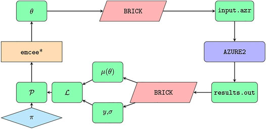
FIGURE 2. Representation of the different roles of emcee, BRICK, and AZURE2 in the Bayesian analysis presented below. The asterisk in the emcee rectangle indicates the starting point of the process.
BRICK is built such that different samplers can be used. The analysis presented in this paper uses emcee, so the details provided in this section will be somewhat specific to it.
When initializing an instance of an EnsembleSampler, the most relevant argument is log_prob_fn, the function that returns the logarithm of the probability. One of the advantages of emcee is that it allows the practitioner to perform arbitrary calculations inside that probability function. That function must meet only two requirements: (1) take an array of floating point numbers that represents the vector in parameter space and (2) return a floating point number that represents the logarithm of the probability associated with that array. In between those two steps, one is free to perform whatever calculations one needs. This can be seen on the left-hand side of Figure 2. The parameter-space vector, θ, is output from emcee. The logarithm of the probability at that point,
The primary tasks that BRICK accomplishes are (1) translating θ into a format that AZURE2 can read and (2) reading the output from AZURE2 such that a
BRICK accesses the AZURE2 CLI through the Python module subprocess. But prior to that, BRICK must map the values in θ to the proper locations in the input file. This is accomplished by reading the <levels> and <sectionsData> sections of the input file. BRICK reads the appropriate parameters and flags looking for varied parameters. As they are found, their locations are stored. When a new θ is proposed, BRICK creates a new input file and maps the values in θ to the varied parameter locations. Then AZURE2 is called with the newly generated input file. The output from AZURE2 is written to a sequence of files in the output directory by default. Those files are read and the predictions, μ, and experimental data, y, are extracted. A likelihood is then constructed. Under the assumption that the uncertainties associated with y are uncorrelated and normally distributed, this is a multivariate Gaussian distribution. Accompanied by a list of prior distributions corresponding to the preexisting knowledge of the sampled parameters, a posterior is finally constructed and passed back to emcee.
Initially, this process was built in a single-threaded manner. As emcee is a ensemble sampler, efficient exploration of the posterior relies heavily on many, simultaneous walkers. In order to scale this beyond the most basic calculations, we modified our implementation to allow each walker to write its own input file and read from its own output directory. Inside the log-probability function, there is no access to any kind of walker identifier, so each walker generates a file-space that is uniquely identified by an eight-character random string. This allows each walker to work independently, so on systems where many cores are available, each walker can have a dedicated core. Or at least the time spent waiting for CPU time is minimized. This also allows for an increased number of walkers, which is a common tactic used to decrease autocorrelation time.
The starting point for the R-matrix model used here was that of deBoer et al. [7]. In that work, ten levels were used with three particle pairs (3He+α, 7Be+γ0, and 7Be+γ1) for a total of 16 R-matrix fit parameters. Initial MCMC calculations showed that a 7/2− background level used in deBoer et al. [7] was not statistically significant, and was thus dropped from the calculation. This already demonstrated one of the powerful feature of this type of MCMC analysis, it provided a clear identification of redundant fit parameters. Likewise, we verified that the exact placement of many of the background levels did not effect the fit results, as long as they were placed at sufficiently high energies. The exception to this was the 5/2− background level, placed at 7 MeV. Because there are two real levels at Ex = 6.73 and 7.21 MeV in 7Be, this background level needed to be placed close to their energies. It was found that this single background level was sufficient to model both the contributions from these levels and additional higher energy 5/2− levels. The R-matrix model used here thus consisted of nine levels, three particle pairs, and 16 R-matrix fit parameters as summarized in Table 1.
Because this is a Bayesian analysis, we must choose priors for all R-matrix parameters. We have chosen to use uninformative, uniform priors. However, the signs of the reduced width amplitudes (that is the interference solution), which are implemented in AZURE2 by the signs of the partial widths, were determined by the initial best χ2 fit using AZURE2. In this case, a unique interference solution was found. This may not always be the case: sometimes other interference solutions may be possible. The emcee sampler may then not be able to easily find these other interference solutions in the parameter space. It seems to be likely that in cases where different interference solutions are possible, each one will require a separate emcee analysis.
One common circumstance where a Bayesian analysis will improve on previous uncertainty estimates is in the ability to give priors for bound state level parameters determined from transfer studies. Unfortunately, in the case of the 7Be system, there is limited information available for the bound state α-particle ANCs. A recent first measurement has been reported by Kiss et al. [59], but the ANCs are rather discrepant from those found from this and past R-matrix analyses of capture data. This inconsistency has not been investigated here, but needs to be addressed in future work. If reliable bound-state ANC determinations become available, that are independent of the capture and scattering data, it provides a path to further decrease the uncertainty in the low energy S-factor extrapolation. One could also adopt priors on the ANCs from ab initio calculations, although we have not done so.
It is also tempting to implement more constraining priors into the R-matrix analysis from a compilation like the National Nuclear Data Center or the TUNL Nuclear Data Project [60]. However, great care must be taken to understand the source of the values and uncertainties when weighted averages are used to determine adopted values for level parameters in these compilations. In particular, past analysis of the data being fit in the R-matrix analysis may be a contributor to the evaluation values. Thus blindly using evaluation level parameters and uncertainties can lead to double counting and an erroneous decrease of uncertainties. It is for this reason that uniform priors on parameters are adopted in the present analysis. The posterior shapes then clearly stem solely from the data sets considered in the R-matrix analysis.
The priors for the R-matrix parameters used in this work are listed in Table 1. In all but one case, level energies are fixed. The exception is the 7/2− level energy which corresponds to the lowest lying 7/2− resonance. The lowest 1/2− and 3/2− levels and the 7/2− level are the only levels inside or below the energy range covered by the analyzed data. All other levels are background levels. For more details of the choices made in formation of the R-matrix model, see Paneru [61]. The distribution formed by the product of these R-matrix priors and priors on the parameters introduced in the next section is the overall prior π shown in Figure 2.
AZURE2 provides a method for the inclusion of a common-mode error for each data set using a modified χ2 function
where cα is the normalization fit parameter, nα is the starting normalization which is set to 1 in the present analysis, f (xα,j) is the differential scattering cross section form the R-matrix, yα,j is the data point value, σα,j is the combined statistical and point-to-point uncertainty of a data point, and
Common-mode errors are implemented in the present analysis in BRICK, outside of AZURE2, i.e., the common-mode errors are applied to the AZURE2 output. In BRICK the R-matrix parameter set θR is augmented by a set of normalization factors fα and energy shifts, ΔE,α. (At present energy shifts are only implemented for scattering data.) The overall parameter set θ is then the union of the set θR and {fα, ΔE,α}. The likelihood
where we have omitted overall factors that do not affect the parameter estimation. Here xjα represents the kinematics of the jth data point in data set α. For scattering data sets, xjα defines the energy and angle at which the measurement was made. In those cases exclusively, ΔE,α is added to the energy. σjα is the combined statistical and point-to-point uncertainty of the corresponding datum, yjα. Nα is the number of points in data set α, and the product over α runs over all the sets that have independent common-mode errors.
The priors on the fα’s are specified by the BRICK user. If a Gaussian prior centered at 1 with a width equal to the common-mode error reported in the original experimental publication is employed for the fα’s, then the product of that prior on the normalization factors and the likelihood Eq. 2 has the same maximum value as the “extended likelihood” corresponding to Eq. 1, that is used to estimate the fα’s in the frequentist framework implemented in AZURE2.
In our analysis of the 3He(α,α)3He and 3He(α,γ)7Be reactions, we adopted such a Gaussian prior, truncated to exclude negative values of the cross section. We used a different fα for each energy bin in the SONIK data, detailed in Section 4.2, with the widths of the prior given by the common-mode errors stated in Table 2. The common-mode error associated with the Barnard data, described in Section 4.1, is taken to be 5%. The width of the priors for the fα’s to be applied to the capture data, discussed in Section 4.3, are specified by the common-mode errors listed in Table 3. All normalization-factor priors are of the form
where
and N (μ, σ2) represents a Gaussian distribution centered at μ with a variance of σ2.

TABLE 3. Details of the capture data considered in this work: number of data points, energy ranges, and common-mode errors (δcommon). Energies are given the laboratory frame.
BRICK also has the capability of estimating (overall) beam-energy shifts in a particular data set. This is implemented as another parameter to be estimated ΔE,α. This parameter affects all the AZURE2 evaluations for data set α. BRICK implements the energy shift by generating a different input and data files for each value of ΔE,α under consideration. The flowchart of Figure 2 is thus not strictly accurate when this feature is included. Gaussian priors were defined, centered at zero, on possible energy shifts for the SONIK data and the Barnard data. The widths of the priors are based on information in the original papers, as summarized in Sections 4.1, 4.2. For the SONIK data, the energy-shift parameter’s prior has a standard deviation of 3 keV, based on the energy uncertainty quoted in Paneru et al. [54]. Barnard et al. [53] cites a much larger uncertainty of 20–40 keV, depending upon the energy. The standard deviation of the prior on the ΔE parameter is taken to be 40 keV for this data set, a much larger value than for the SONIK data. It should be noted that the energy uncertainty for the Barnard data set is not a constant, but it is not possible to improve our modeling of this uncertainty due to the lack of documentation of its origin.
Measurements of the elastic scattering products resulting from a 3He beam incident on a 4He target were reported in 1964 by Barnard et al. [53], for 2.4 ≤ E [3He, lab] ≤ 5.7 MeV (1.4 ≤ Ec. m. ≤ 3.3 MeV). The experiment provides excitation functions of differential cross section at eight center-of-mass (c.m.) angles covering 31.55° ≤ θ[3He, lab] ≤ 91.94° (54.77° ≤ θc.m. ≤ 140.8°). The systematic uncertainty in the measurements is estimated to be 5%. Detailed point-to-point uncertainties are not given, but are stated to be about 3%. The measurements are subject to a significant energy uncertainty, estimated to be 20 keV below E [3He, lab] = 4 MeV and 40 keV above that energy. It was also noted by the authors that their beam energy was only reproducible to the level of 20 keV. In total, there are 646 data points collected at 577 unique energies. The data were obtained from EXFOR in the fall of 2021 and converted into the laboratory frame when necessary. All eight angles were included. The previous analysis by deBoer et al. [7] omitted the largest angle.
A new measurement of 3He+α elastic scattering was performed at TRIUMF using the SONIK [61,63] target and detector system. SONIK was filled with 4He gas maintained at a typical pressure of 5 Torr bombarded with 3He with a beam intensity of about 1012 pps. Elastic scattering cross sections were measured at nine different energies from Ec. m. = 0.38–3.13 MeV. SONIK covers an angular range of 30° < θc.m. < 139°—a markedly larger range than previous measurements. The detectors in SONIK were arranged such that they observed three different points, termed interaction regions, in the gas target along the beam direction. When the beam traversed the gas target it lost energy, so the bombarding energy, and therefore the scattering energy, was slightly different in each of the three interaction regions.
As we will explore further below, the results for the differential scattering cross section from this measurement are consistent with previous determinations but have better precision. The data also extend to markedly lower energies. The uncertainties with this measurement are well quantified and are presented in Paneru et al. [54]. A separate normalization uncertainty is determined for each beam energy. These normalization uncertainties range from 4.1 to 9.8%.
The data selection [39–42,44,45] for the 3He (α,γ)7Be reaction for this work follows that of previous recent works [7,22,47,64]. Note that the LUNA measurements of Gyürky et al. [65] and Confortola et al. [66] are collected in Costantini et al. [41]. The combined data sets cover a wide energy range from Ec. m. = 94–3130 keV, but still remain below the proton decay threshold. Older data are not included due to a long history of discrepancies, which manifested as differences between experiments that used either direct detection of γ-rays or the activation technique. More recent measurements have achieved consistency resulting from improved experimental techniques by performing consistency check measurements using both direct detection of γ-rays and the activation technique [47]. Details about the capture data sets, including common-mode errors for cross sections, are listed in Table 3.
Two distinct data models are analyzed here,
The results of our analysis are presented here in two subsections. The first discusses results in the energy regime of the data that was analyzed. The second computes extrapolated quantities—observables that lie in energy regimes outside those covered by the analyzed data.
First we examine the extent to which our results match experimental data. We do this by comparing predicted and measured observables.
Figure 3 shows the total capture S-factor data alongside bands representing 68% intervals from the analyses of both data models,
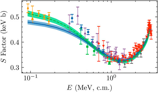
FIGURE 3. Total capture S factor from Seattle [2] (blue circles) Weizmann [42] (green squares), LUNA [41] (orange diamonds), ERNA [45] (red, downward-pointing triangles), Notre Dame [39] (purple, upward-pointing triangles), and ATOMKI [44] (black stars) data sets are shown with reported error bars.
The branching ratio, defined as the ratio of the excited-state cross section to the ground-state cross section, results for both data models—
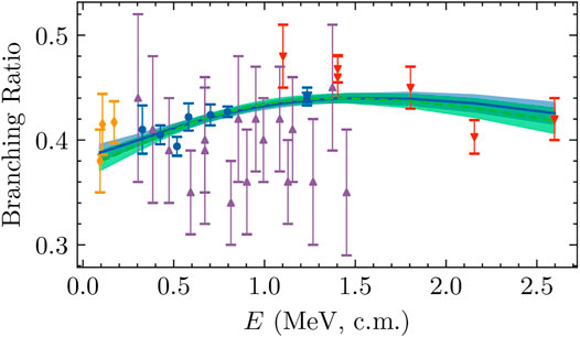
FIGURE 4. The branching ratio predictions are shown alongside the four analyzed branching ratio data sets: Seattle [2], LUNA [41], ERNA [45], and Notre Dame [39]. Colors, symbols, and line styles are the same as Panel 3. Bands indicate 68% intervals.
The differential cross sections from the SONIK [54] and Barnard et al. [53] measurements are shown in Figures 5 and 6, respectively, with the predictions from our analyses. In all cases, both analyses reproduce the data to high accuracy. However, the
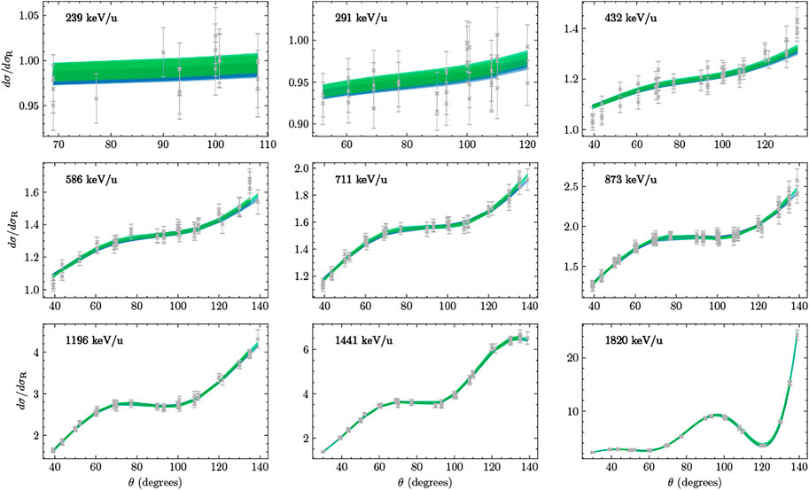
FIGURE 5. Angular dependence of the differential cross sections of Paneru et al. [54] are shown relative to the Rutherford prediction with grey x’s and error bars. Each panel includes the measurements from three interaction regions [61]. Bands indicate 68% intervals. Green bands are generated for the analysis of

FIGURE 6. Differential cross section as a function of energy as reported in Barnard et al. [53], shown as grey x’s with error bars. Blue bands represent the 68% intervals generated from the
Separate corner plots for each data model are provided in the Supplemental Material. There are notable differences in several R-matrix parameters. In particular, the
The
All parameters shown in Figure 7 are well-constrained. By comparing to the prior distributions listed in Table 1, one can see the dominance of the data’s influence over the information in the prior: all posterior distributions are markedly narrower than the priors chosen. As discussed in Section 3.2, several R-matrix-model iterations were taken to remove redundant parameters.
The correlation matrix of the R-matrix parameters is shown in Figure 8. The figure represents an approximation of the full information contained in the corner plot given in the Supplemental Material. There, significant, often-nonlinear, correlations are observable between several pairs of R-matrix parameters. In particular, the influence of the ANCs over the entire R-matrix parameter space, either directly or indirectly, means that it is very important for scattering data to have well-defined uncertainties over its full energy range.
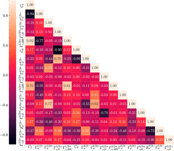
FIGURE 8. Correlation matrix of R-matrix parameters for the
The normalization factors applied to the theory predictions for each of the total capture data sets are shown for both data models in Figure 9. The comparison reveals good agreement between
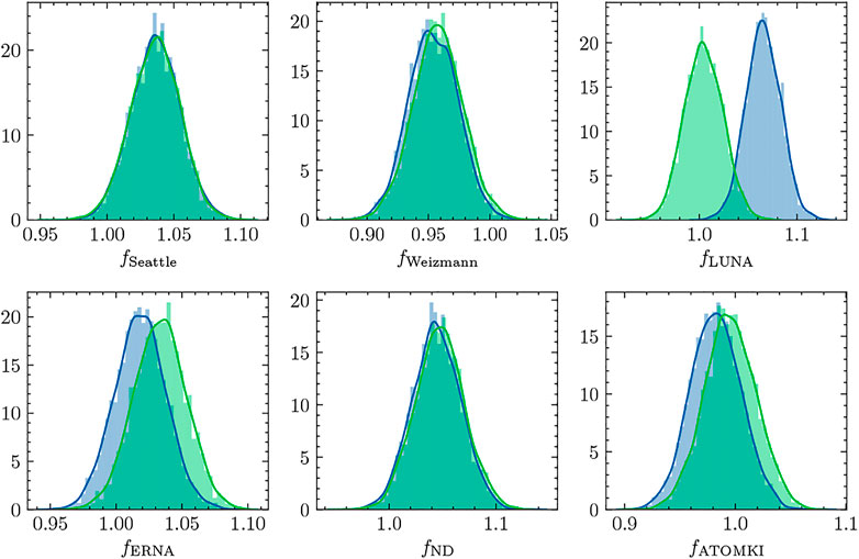
FIGURE 9. The normalization factors applied to the total cross section predicted by our R-matrix model are compared for each of the total capture data sets (Seattle [2] Weizmann [42], LUNA [41], ERNA [45], Notre Dame [39], and ATOMKI [44]).
The normalization factors applied to the theory predictions for each of the SONIK energies are shown in Figure 10. When the data of Barnard et al. [53] are included in the analysis, the SONIK normalization factors are significantly larger. This effect is systematically apparent at lower energies. In more than half the cases, the
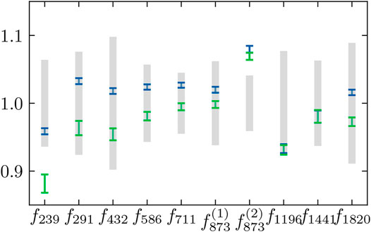
FIGURE 10. Summaries of the normalization factor posteriors for each SONIK [54] data set are shown for
The posteriors for fBarnard and the energy shifts for both the Barnard et al. [53] and SONIK [54] data sets (see Section 3.3) are shown in Figure 11. The result for fBarnard is

FIGURE 11. Posteriors of the normalization factor applied to the Barnard data and the energy shifts introduced to the Barnard et al. [53] and SONIK [54] data sets. The Barnard normalization factor is applied to the theory prediction. Energy shifts are presented in keV. These results were obtained exclusively with the
The ANCs corresponding to the two bound 7Be states are of particular interest for extrapolating threshold quantities. First, we point out that the inclusion of scattering data significantly reduces the uncertainty of the ANCs. Our posterior is much narrower than that obtained using capture-only data in Zhang et al. [22]. This highlights the importance of scattering data in constraining bound-state properties and the amplitudes associated with transitions to them.
Second, the choice of scattering data set matters. The C1 results from analyzing
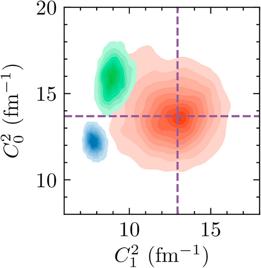
FIGURE 12. The two-dimensional posterior of the squares of the ANCs, C0 and C1. Results for
The Coulomb-modified effective range function is given in Hamilton et al. [67] and van Haeringen [68] as
where k is the relative momentum, ℓ is the angular momentum, η is the Sommerfeld parameter, Γ is the gamma function, uℓ(η) is given by
with
and Ψ representing the digamma function [69]. This effective range function is an analytic function of E (or k2) near E = 0. From the phase shifts, obtained with BRICK, calculated over a range of low momenta, one can fit the scattering length, a0, and effective range, r0, according to the low-energy expansion
Our calculation involves 70 equally spaced phase shifts over a range of low energies from 0.57 keV to 3.93 MeV. The results are used to evaluate the effective range function defined by Eq. 5. The energy dependence is then fit to Eq. 10 using a non-linear least squares fit. In addition to a0 and r0 defined in Eq. 5, the shape parameter at
The results from
Figure 14 shows a comparison of the scattering lengths obtained from the
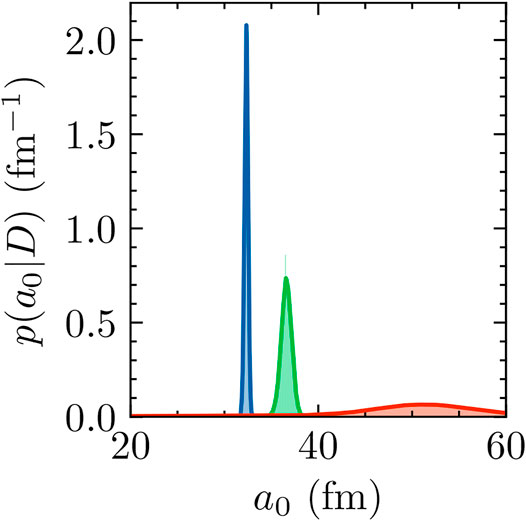
FIGURE 14. a0 posteriors obtained from

TABLE 4. A summary of the posteriors of the extrapolated quantities. Where possible, results from other anlayses are included.
The
The total capture S factor at zero energy was extrapolated by evaluating the S factor at 100 evenly spaced points between 1 and 100 keV, constructing a cubic-polynomial interpolation function to represent the calculations, and evaluating that function at zero energy. Errors from the interpolation/extrapolation process are negligible when compared to contributions from parameter uncertainties. The results are shown alongside previous results in Figure 15. As expected from the different low-energy behaviors shown in Figure 3, the
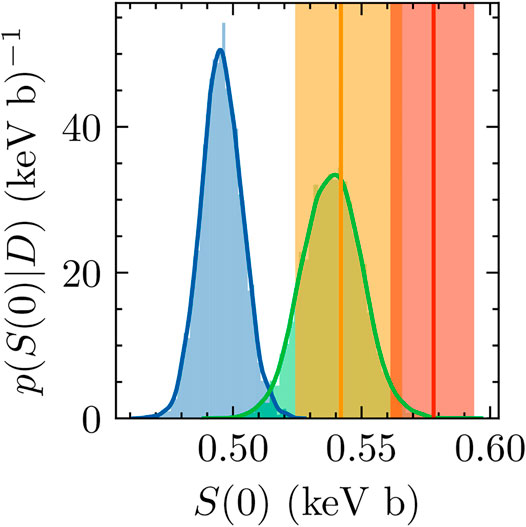
FIGURE 15. Extrapolated S(0) posteriors from the analyses of both
Insights into the relevance of parameters can be obtained by examining the correlations between them. In Figure 16, the correlations between S(0) and a0,
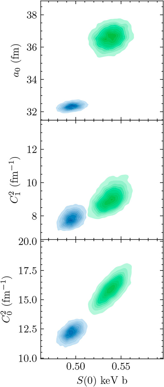
FIGURE 16. Two-dimensional posteriors are presented for the analyses of both
We have described and applied the Bayesian R-matrix Inference Code Kit (BRICK), which facilitates communication between the phenomenological R-matrix code AZURE2 [3] and a Markov Chain Monte Carlo (MCMC) sampler such as emcee [36]. It thereby enables MCMC sampling of the joint posterior probability density function (pdf) for the R-matrix parameters and normalization factors. With samples that represent such a posterior in hand, the computation of the pdf for any quantity that can be calculated in the R-matrix formalism is straightforward.
While BRICK is a general tool, we have also provided an example of its application to an R-matrix fit of 3He-α scattering and the 3He (α,γ)7Be capture reaction data, in order to make inferences about the 7Be system. This application was partly motivated by the availability of a new 3He-α scattering data set obtained using the SONIK detector at TRIUMF [61] following the suggestion of deBoer et al. [7]. These data have more carefully quantified uncertainties than a previous measurement by Barnard et al. [53]. Our study shows this motivation was well justified, finding discrepant values for extrapolated quantifies when the data of Barnard et al. [53] were included. Our analysis of the SONIK data shows consistency between them and capture data, producing an S factor in accord with analyses of capture data alone: our final
This emphasizes the importance of detailed uncertainty quantification when data sets are to be used for accurate inference of extrapolated quantities, where Barnard et al. [53] does not include these kinds of details regarding the experiment. This makes the tension between the Barnard et al. [53] and SONIK data regarding S(0) difficult to resolve, thus the Barnard et al. [53] data may need to be omitted from future evaluations. We emphasize, though, that these previous data were invaluable in advancing our understanding of the 7Be system to its current state, but data with more well defined uncertainties are needed for current applications.
Zhang, Nollett, and Phillips pointed out that the s-wave 3He-α scattering length is correlated with this result [22]. The
Improvements in the analyses presented here could occur if there were:
• Better documentation of the energy dependence of systematic uncertainties in published data sets. The Bayesian formalism that underlies BRICK allows systematic uncertainties with any correlation structure to be incorporated into the analysis.
• Improved understanding of the way theory uncertainties in the phenomenological R-matrix formalism affect the extrapolation of data.
• Detailed modern data with full uncertainty quantification in the vicinity of the 7/2− resonance. This may help resolve some of the ambiguities in results between the
• Ab initio constraints, e.g., on ANCs could be incorporated in the analysis.
• Data from transfer reactions that provided complementary information on the 7Be ANCs.
Future applications of BRICK could include posteriors for astrophysical reaction rates. This would enhance BRICK’s utility as a tool for performing detailed uncertainty quantification on nuclear reactions, especially those of astrophysical interest. AZURE2 already includes the necessary functionality. Implementing this feature ought to be a straightforward process.
Publicly available datasets were analyzed in this study. This data can be found here: Data are available on the EXFOR data repository https://www-nds.iaea.org/exfor/. The data measured at TRIUMF using the SONIK gas target will be available in an upcoming publication.
CB and DP formulated the conceptual design of the project. DO was the author of the BRICK code and was the author of the first draft of the manuscript. RD consulted DO to facilitate the interface of the BRICK with AZURE2 codes, perform benchmark calculations, and the calculations for the 7Be system. SP supplied their experimental data for the calculations and consulted on its analysis. CB and RD collected and interpreted past experimental data from the literature. All authors contributed to the critical discussions of the research, writing, revising, reading, and approving the submitted manuscript.
This work was supported by the U.S. Department of Energy, National Nuclear Security Agency under Award DE-NA0003883, and Office of Science, Office of Nuclear Physics, under Award DE-FG02-93 ER-40756, as well as by the National Science Foundation under grants OAC-2004601 (CSSI program, BAND collaboration), PHY-2011890 (University of Notre Dame Nuclear Science Laboratory), and PHY-1430152 (the Joint Institute for Nuclear Astrophysics - Center for the Evolution of the Elements). This research utilized resources from the Notre Dame Center for Research Computing.
The authors declare that the research was conducted in the absence of any commercial or financial relationships that could be construed as a potential conflict of interest.
All claims expressed in this article are solely those of the authors and do not necessarily represent those of their affiliated organizations, or those of the publisher, the editors and the reviewers. Any product that may be evaluated in this article, or claim that may be made by its manufacturer, is not guaranteed or endorsed by the publisher.
We thank Maheshwor Poudel and Xilin Zhang for helpful discussions.
The Supplementary Material for this article can be found online at: https://www.frontiersin.org/articles/10.3389/fphy.2022.888476/full#supplementary-material
1We use slightly different common-mode uncertainty estimates in our prior definitions than those listed in [61]. This update will be reflected in a forthcoming publication by the SONIK collaboration [54].
1. Lane AM, Thomas RG. R-matrix Theory of Nuclear Reactions. Rev Mod Phys (1958) 30:257–353. doi:10.1103/RevModPhys.30.257
2. Brown DA, Chadwick MB, Capote R, Kahler AC, Trkov A, Herman MW, et al. ENDF/B-VIII.0: The 8 Th Major Release of the Nuclear Reaction Data Library with CIELO-Project Cross Sections, New Standards and Thermal Scattering Data. Nucl Data Sheets (2018) 148:1–142. doi:10.1016/j.nds.2018.02.001
3. Azuma RE, Uberseder E, Simpson EC, Brune CR, Costantini H, de Boer RJ, et al. AZURE: AnR-Matrix Code for Nuclear Astrophysics. Phys Rev C (2010) 81:045805. doi:10.1103/PhysRevC.81.045805
4. Descouvemont P, Adahchour A, Angulo C, Coc A, Vangioni-Flam E. Big-Bang Reaction Rates within the R-Matrix Model. Nucl Phys ANuclei Cosmos VIII (2005) 758:783–6. doi:10.1016/j.nuclphysa.2005.05.140
5.ENSDF. From ENSDF Database as of April 12, 2022 (2022). Version available from: http://www.nndc.bnl.gov/ensarchivals/ (Accessed January 10, 2021).
6. Smith DL, Badikov SA, Gai EV, Oh S-Y, T. Kawano NML, Pronyaev VG. Perspectives on Peelle’s Pertinent Puzzle. In: International Evaluation of Neutron Cross-Section Standards. Wagramer Strasse 5, P.O. Box 100, 1400 Vienna, Austria: International Atomic Energy Agency (2007). p. 46–83.
7. deBoer RJ, Görres J, Smith K, Uberseder E, Wiescher M, Kontos A, et al. Monte Carlo Uncertainty of theHe3(α,γ)Be7reaction Rate. Phys Rev C (2014) 90:035804. doi:10.1103/PhysRevC.90.035804
8. Schindler MR, Phillips DR. Bayesian Methods for Parameter Estimation in Effective Field Theories. Ann Phys (2009) 324:682–708. doi:10.1016/j.aop.2008.09.003
9. Furnstahl RJ, Phillips DR, Wesolowski S. A Recipe for EFT Uncertainty Quantification in Nuclear Physics. J Phys G: Nucl Part Phys (2015) 42:034028. doi:10.1088/0954-3899/42/3/034028
10. Furnstahl RJ, Klco N, Phillips DR, Wesolowski S. Quantifying Truncation Errors in Effective Field Theory. Phys Rev C (2015) 92:024005. doi:10.1103/PhysRevC.92.024005
11. Zhang X, Nollett KM, Phillips DR. Halo Effective Field Theory Constrains the Solar 7Be + P → 8B + γ Rate. Phys Lett B (2015) 751:535–40. doi:10.1016/j.physletb.2015.11.005
12. Melendez JA, Wesolowski S, Furnstahl RJ. Bayesian Truncation Errors in Chiral Effective Field Theory: Nucleon-Nucleon Observables. Phys Rev C (2017) 96:024003. doi:10.1103/PhysRevC.96.024003
13. Wesolowski S, Furnstahl RJ, Melendez JA, Phillips DR. Exploring Bayesian Parameter Estimation for Chiral Effective Field Theory Using Nucleon-Nucleon Phase Shifts. J Phys G: Nucl Part Phys (2019) 46:045102. doi:10.1088/1361-6471/aaf5fc
14. Neufcourt L, Cao Y, Giuliani S, Nazarewicz W, Olsen E, Tarasov OB. Beyond the Proton Drip Line: Bayesian Analysis of Proton-Emitting Nuclei. Phys Rev C (2020) 101:014319. doi:10.1103/PhysRevC.101.014319
15. Neufcourt L, Cao Y, Nazarewicz W, Olsen E, Viens F. Neutron Drip Line in the Ca Region from Bayesian Model Averaging. Phys Rev Lett (2019) 122:062502. doi:10.1103/PhysRevLett.122.062502
16. King GB, Lovell AE, Neufcourt L, Nunes FM. Direct Comparison between Bayesian and Frequentist Uncertainty Quantification for Nuclear Reactions. Phys Rev Lett (2019) 122:232502. doi:10.1103/PhysRevLett.122.232502
17. Melendez JA, Furnstahl RJ, Phillips DR, Pratola MT, Wesolowski S. Quantifying Correlated Truncation Errors in Effective Field Theory. Phys Rev C (2019) 100:044001. doi:10.1103/PhysRevC.100.044001
18. Filin AA, Baru V, Epelbaum E, Krebs H, Möller D, Reinert P. Extraction of the Neutron Charge Radius from a Precision Calculation of the Deuteron Structure Radius. Phys Rev Lett (2020) 124:082501. doi:10.1103/PhysRevLett.124.082501
19. Drischler C, Furnstahl RJ, Melendez JA, Phillips DR. How Well Do We Know the Neutron-Matter Equation of State at the Densities inside Neutron Stars? A Bayesian Approach with Correlated Uncertainties. Phys Rev Lett (2020) 125:202702. doi:10.1103/PhysRevLett.125.202702
20. Drischler C, Melendez JA, Furnstahl RJ, Phillips DR. Quantifying Uncertainties and Correlations in the Nuclear-Matter Equation of State. Phys Rev C (2020) 102:054315. doi:10.1103/PhysRevC.102.054315
21. Premarathna P, Rupak G. Bayesian Analysis of Capture Reactions $$\varvec{^3}\hbox {He}\varvec{(\alpha ,\gamma )^7}\hbox {Be}$$ and $$\varvec{^3}\hbox {H}\varvec{(\alpha ,\gamma )^7}\hbox {Li}$$. Eur Phys J A (2020) 56:166. doi:10.1140/epja/s10050-020-00113-z
22. Zhang X, Nollett KM, Phillips DR. S-factor and Scattering-Parameter Extractions from ${}^{3}\mathrm{He}+{}^{4}\mathrm{He}{ \rightarrow }^{7}\mathrm{Be}+\gamma $. J Phys G: Nucl Part Phys (2020) 47:054002. doi:10.1088/1361-6471/ab6a71
23. Filin AA, Möller D, Baru V, Epelbaum E, Krebs H, Reinert P. High-accuracy Calculation of the Deuteron Charge and Quadrupole Form Factors in Chiral Effective Field Theory. Phys Rev C (2021) 103:024313. doi:10.1103/PhysRevC.103.024313
24. Schunck N, Quinlan KR, Bernstein J. A Bayesian Analysis of Nuclear Deformation Properties with Skyrme Energy Functionals. J Phys G: Nucl Part Phys (2020) 47:104002. doi:10.1088/1361-6471/aba4fa
25. Neufcourt L, Cao Y, Giuliani SA, Nazarewicz W, Olsen E, Tarasov OB. Quantified Limits of the Nuclear Landscape. Phys Rev C (2020) 101:044307. doi:10.1103/PhysRevC.101.044307
26. Everett D, Ke W, Paquet J-F, Vujanovic G, Bass SA, Du L, et al. Multisystem Bayesian Constraints on the Transport Coefficients of QCD Matter. Phys Rev C (2021) 103:054904. doi:10.1103/PhysRevC.103.054904
27. Catacora-Rios M, King GB, Lovell AE, Nunes FM. Statistical Tools for a Better Optical Model. Phys Rev C (2021) 104:064611. doi:10.1103/PhysRevC.104.064611
28. Reinert P, Krebs H, Epelbaum E. Precision Determination of Pion-Nucleon Coupling Constants Using Effective Field Theory. Phys Rev Lett (2021) 126:092501. doi:10.1103/PhysRevLett.126.092501
29. Phillips DR, Furnstahl RJ, Heinz U, Maiti T, Nazarewicz W, Nunes FM, et al. Get on the BAND Wagon: A Bayesian Framework for Quantifying Model Uncertainties in Nuclear Dynamics. J Phys G: Nucl Part Phys (2021) 48:072001. doi:10.1088/1361-6471/abf1df
30. Wesolowski S, Svensson I, Ekström A, Forssén C, Furnstahl RJ, Melendez JA, et al. Rigorous Constraints on Three-Nucleon Forces in Chiral Effective Field Theory from Fast and Accurate Calculations of Few-Body Observables. Phys Rev C (2021) 104:064001. doi:10.1103/PhysRevC.104.064001
32. Xu J, Zhang Z, Li B-A. Bayesian Uncertainty Quantification for Nuclear Matter Incompressibility. Phys Rev C (2021) 104:054324. doi:10.1103/PhysRevC.104.054324
33. Cao S, Chen Y, Coleman J, Mulligan J, Jacobs PM, Soltz RA, et al. Determining the Jet Transport Coefficient q̂ from Inclusive Hadron Suppression Measurements Using Bayesian Parameter Estimation from Inclusive Hadron Suppression Measurements Using Bayesian Parameter Estimation. Phys Rev C (2021) 104:024905. doi:10.1103/PhysRevC.104.024905
34. Hamaker A, Leistenschneider E, Jain R, Bollen G, Giuliani SA, Lund K, et al. Precision Mass Measurement of Lightweight Self-Conjugate Nucleus 80Zr. Nat Phys (2021) 17:1408–12. doi:10.1038/s41567-021-01395-w
36. Foreman-Mackey D, Hogg DW, Lang D, Goodman J. Emcee: The MCMC Hammer. Publications Astronomical Soc Pac (2013) 125:306–12. doi:10.1086/670067
37. Bahcall JN, Ulrich RK. Solar Models, Neutrino Experiments, and Helioseismology. Rev Mod Phys (1988) 60:297–372. doi:10.1103/RevModPhys.60.297
38. Cyburt RH, Fields BD, Olive KA, Yeh T-H. Big Bang Nucleosynthesis: Present Status. Rev Mod Phys (2016) 88:015004. doi:10.1103/RevModPhys.88.015004
39. Kontos A, Uberseder E, deBoer R, Görres J, Akers C, Best A, et al. AstrophysicalSfactor of 3He(α,γ)7Be. Phys Rev C (2013) 87:065804. doi:10.1103/PhysRevC.87.065804
40. Brown TAD, Bordeanu C, Snover KA, Storm DW, Melconian D, Sallaska AL, et al. 3He+4He→7Be astrophysical S factor. Phys Rev C (2007) 76:055801. doi:10.1103/PhysRevC.76.055801
41. Costantini H, Bemmerer D, Confortola F, Formicola A, Gyürky G, Bezzon P, et al. The S-Factor at Solar Energies: The Prompt γ experiment at LUNA. Nucl Phys A (2008) 814:144–58. doi:10.1016/j.nuclphysa.2008.09.014
42. Singh BS, Hass M, Nir-El Y, Haquin G. New Precision Measurement of the 3He(4He, γ) 7Be Cross Section Cross Section. Phys Rev Lett (2004) 93:262503. doi:10.1103/PhysRevLett.93.262503
43. Carmona-Gallardo M, Nara Singh BS, Borge MJG, Briz JA, Cubero M, Fulton BR, et al. New Measurement of the 3He(α,γ)7Be Cross Section at Medium Energies. Phys Rev C (2012) 86:032801. doi:10.1103/PhysRevC.86.032801
44. Bordeanu C, Gyürky G, Halász Z, Szücs T, Kiss GG, Elekes Z, et al. Activation Measurement of the Reaction Cross Section at High Energies. Nucl Phys A (2013) 908:1–11. doi:10.1016/j.nuclphysa.2013.03.012
45. Di Leva A, Gialanella L, Kunz R, Rogalla D, Schürmann D, Strieder F, et al. Stellar and Primordial Nucleosynthesis of 7Be: Measurement of 3He(α,γ)7Be. Phys Rev Lett (2009) 102:232502. doi:10.1103/PhysRevLett.102.232502
46. Szücs T, Kiss GG, Gyürky G, Halász Z, Szegedi TN, Fülöp Z. Cross Section of 3He(α,γ)7Be Around the 7Be Proton Separation Threshold. Phys Rev C (2019) 99:055804. doi:10.1103/PhysRevC.99.055804
47. Adelberger EG, García A, Robertson RGH, Snover KA, Balantekin AB, Heeger K, et al. Solar Fusion Cross Sections. II. Theppchain and CNO Cycles. Rev Mod Phys (2011) 83:195–245. doi:10.1103/RevModPhys.83.195
48. Tursunov EM, Turakulov SA, Kadyrov AS. Analysis of the 3He(α,γ)7Be and 3H(α,γ)7Li Astrophysical Direct Capture Reactions in a Modified Potential-Model Approach. Nucl Phys A (2021) 1006:122108. doi:10.1016/j.nuclphysa.2020.122108
49. Nollett KM. Radiativeα-capture Cross Sections from Realistic Nucleon-Nucleon Interactions and Variational Monte Carlo Wave Functions. Phys Rev C (2001) 63:054002. doi:10.1103/PhysRevC.63.054002
50. Neff T. Microscopic Calculation of the 3He(α,γ)7Be and 3H(α,γ)7Li Capture Cross Sections Using Realistic Interactions. Phys Rev Lett (2011) 106:042502. doi:10.1103/PhysRevLett.106.042502
51. Dohet-Eraly J, Navrátil P, Quaglioni S, Horiuchi W, Hupin G, Raimondi F. 3He(α,γ)7Be and 3H(α,γ)7Li Astrophysical S Factors from the No-Core Shell Model with Continuum. Phys Lett B (2016) 757:430–6. doi:10.1016/j.physletb.2016.04.021
52. Vorabbi M, Navrátil P, Quaglioni S, Hupin G. 7Be and 7Li Nuclei within the No-Core Shell Model with Continuum. Phys Rev C (2019) 100:024304. doi:10.1103/PhysRevC.100.024304
53. Barnard ACL, Jones CM, Weil JL. Elastic Scattering of 2-11 MeV Protons by He4. Nucl Phys (1964) 50:604–20. doi:10.1016/0029-5582(64)90233-0
54. Paneru SN, Brune CR, Connolly D, Karpesky J, Davids B, Ruiz C, et al. Elastic Scattering of 3He + 4He with SONIK (2022). Unpublished.
55. deBoer RJ, Görres J, Wiescher M, Azuma RE, Best A, Brune CR, et al. The 12C(α,γ)16O Reaction and its Implications for Stellar Helium Burning. Rev Mod Phys (2017) 89:035007. doi:10.1103/RevModPhys.89.035007
56. Brune CR. Alternative Parametrization ofR-Matrix Theory. Phys Rev C (2002) 66:044611. doi:10.1103/PhysRevC.66.044611
57. Mukhamedzhanov AM, Tribble RE. Connection between Asymptotic Normalization Coefficients, Subthreshold Bound States, and Resonances. Phys Rev C (1999) 59:3418–24. doi:10.1103/PhysRevC.59.3418
58. Mukhamedzhanov AM, Gagliardi CA, Tribble RE. Asymptotic Normalization Coefficients, Spectroscopic Factors, and Direct Radiative Capture Rates. Phys Rev C (2001) 63:024612. doi:10.1103/PhysRevC.63.024612
59. Kiss GG, La Cognata M, Spitaleri C, Yarmukhamedov R, Wiedenhöver I, Baby LT, et al. Astrophysical S-Factor for the 3He(α,γ)7Be Reaction via the Asymptotic Normalization Coefficient (ANC) Method. Phys Lett B (2020) 807:135606. doi:10.1016/j.physletb.2020.135606
60. Tilley DR, Cheves CM, Godwin JL, Hale GM, Hofmann HM, Kelley JH, et al. Energy Levels of Light Nuclei A=5, 6, 7. Nucl Phys A (2002) 708:3–163. doi:10.1016/S0375-9474(02)00597-3
61. Paneru SN. Elastic Scattering of 3He+4He with SONIK. Ph.D. thesis. Athens, OH, USA: Ohio University (2020).
62. D’Agostini G. On the Use of the Covariance Matrix to Fit Correlated Data. Nucl Instr Methods Phys Res Section A: Acc Spectrometers, Detectors Associated Equipment (1994) 346:306–11. doi:10.1016/0168-9002(94)90719-6
63. Connolly D. Radiative Alpha Capture on S34 at Astrophysically Relevant Energies and Design of a Scattering Chamber for High Precision Elastic Scattering Measurements for the DRAGON experiment. Ph.D. thesis. Golden, CO, USA: Colorado School of Mines (2015).
64. Cyburt RH, Davids B. Evaluation of modern 3He(α,γ)7Be data. Phys Rev C (2008) 78:064614. doi:10.1103/PhysRevC.78.064614
65. Gyürky G, Confortola F, Costantini H, Formicola A, Bemmerer D, Bonetti R, et al. 3He(α,γ)7Be cross Section at Low Energies. Phys Rev C (2007) 75:035805. doi:10.1103/PhysRevC.75.035805
66. Confortola F, Bemmerer D, Costantini H, Formicola A, Gyürky G, Bezzon P, et al. AstrophysicalSfactor of the 3He(α,γ)7Be reaction Measured at Low Energy via Detection of Prompt and Delayed γ Rays. Phys Rev C (2007) 75:065803. doi:10.1103/PhysRevC.75.065803
67. Hamilton J, Øverbö I, Tromborg B. Coulomb Corrections in Non-relativistic Scattering. Nucl Phys B (1973) 60:443–77. doi:10.1016/0550-3213(73)90193-4
68. van Haeringen H. T Matrix and Effective Range Function for Coulomb Plus Rational Separable Potentials Especially for I=1. J Math Phys (1977) 18:927–40. doi:10.1063/1.523373
69. Humblet J. Bessel Function Expansions of Coulomb Wave Functions. J Math Phys (1985) 26:656–9. doi:10.1063/1.526602
Keywords: R-matrix, Bayesian uncertainty analysis, nuclear astrophysics, Big Bang nucleosynthesis, asymptotic normalization coefficient
Citation: Odell D, Brune CR, Phillips DR, deBoer RJ and Paneru SN (2022) Performing Bayesian Analyses With AZURE2 Using BRICK: An Application to the 7Be System. Front. Phys. 10:888476. doi: 10.3389/fphy.2022.888476
Received: 02 March 2022; Accepted: 22 April 2022;
Published: 13 June 2022.
Edited by:
Maria Piarulli, Washington University in St. Louis, United StatesReviewed by:
Petr Navratil, TRIUMF, CanadaCopyright © 2022 Odell, Brune, Phillips, deBoer and Paneru. This is an open-access article distributed under the terms of the Creative Commons Attribution License (CC BY). The use, distribution or reproduction in other forums is permitted, provided the original author(s) and the copyright owner(s) are credited and that the original publication in this journal is cited, in accordance with accepted academic practice. No use, distribution or reproduction is permitted which does not comply with these terms.
*Correspondence: Daniel Odell, ZG9kZWxsQG9oaW8uZWR1
Disclaimer: All claims expressed in this article are solely those of the authors and do not necessarily represent those of their affiliated organizations, or those of the publisher, the editors and the reviewers. Any product that may be evaluated in this article or claim that may be made by its manufacturer is not guaranteed or endorsed by the publisher.
Research integrity at Frontiers

Learn more about the work of our research integrity team to safeguard the quality of each article we publish.