- 1Laboratory for Nuclear Science, Massachusetts Institute of Technology, Cambridge, MA, United States
- 2Mathematical Institute, University of St Andrews, St Andrews, UK
- 3Laboratory for Simulation and Modelling, Paul Scherrer Institut, Villigen, Switzerland
We present a novel machine learning-based approach to generate fast-executing virtual radiofrequency quadrupole (RFQ) particle accelerators using surrogate modelling. These could potentially be used as on-line feedback tools during beam commissioning and operation, and to optimize the RFQ beam dynamics design prior to construction. Since surrogate models execute orders of magnitude faster than corresponding physics beam dynamics simulations using standard tools like PARMTEQM and RFQGen, the computational complexity of the multi-objective optimization problem reduces significantly. Ultimately, this presents a computationally inexpensive and time efficient method to perform sensitivity studies and an optimization of the crucial RFQ beam output parameters like transmission and emittances. Two different methods of surrogate model creation (polynomial chaos expansion and neural networks) are discussed and the achieved model accuracy is evaluated for different study cases with gradually increasing complexity, ranging from a simple FODO cell example to the full RFQ optimization. We find that variations of the beam input Twiss parameters can be reproduced well. The prediction of the beam with respect to hardware changes, e.g., the electrode modulation, are challenging on the other hand. We discuss possible reasons for that and elucidate nevertheless existing benefits of the applied method to RFQ beam dynamics design.
1 Introduction
Machine Learning (ML), using statistical methods and Neural Networks (NNs), is quickly becoming a staple of modern computational physics. Their highly successful application in computer vision [1], [2] and the establishment of many software packages that are widely available and standardized (e.g., TensorFlow [3] and Keras [4]) has led to attempts to use ML in almost all fields of science. Particle accelerator physics is no exception, although ML is not as well-established here as in other fields. A few examples of ML in accelerator physics are given in the following. Arguably, the best-established use of ML is image analysis using convolutional neural networks (CNNs). CNNs can be used in beam diagnostics for the analysis of the output of emittance scanners, optical fibers, residual gas monitors, and reconstruction of beam pulse structure [5]. The SwissFEL was tuned using Bayesian optimization [6, 7]. Bayesian optimization, using Gaussian Process models was also used for the Linac Coherent Light Source (LCLS) [8].Another very promising technique, that is also the subject of this paper, is surrogate modelling. We describe the method in detail later. In short, a fast-executing model of a complex system can be produced by training a NN or using Polynomial Chaos Expansion (PCE) on a set of high-fidelity simulations. This fast-executing Surrogate Model (SM) can then be used in an optimization scheme or for on-line feedback during run-time. Some examples of successful use of surrogate models in particle accelerator optimization are given in [9], [10–12], which have demonstrated speedups of one to several orders of magnitude compared to conventional techniques.
To our knowledge, ML has not yet been applied to the design of radiofrequency quadrupole (RFQ) linear accelerators. Here we report our recent results using surrogate modelling to create virtual RFQ models that can be used in several ways:
• Uncertainty Quantification (UQ) [13] of the RFQ with respect to input beam variations or RFQ settings during run-time.
• Prediction of output beam parameters from a given set of input beam parameters. The SM becomes a virtual accelerator, ideal as tuning and commissioning aid.
• Design and optimization of the RFQ hardware. Based on the success as a virtual accelerator, we also tested the SM technique as a hardware optimization tool.
The findings in this paper are fully transferable to other RFQs.
1.1 Particle Physics Motivation for This Work
The motivation for this work lies in the IsoDAR project [13]; [14,15], a proposed search for exotic neutrinos. These are hypothesized cousins to the three known standard model neutrinos and could explain anomalies seen in the neutrino oscillation experiments of the past 3 decades [16].
To reach discovery-level sensitivity
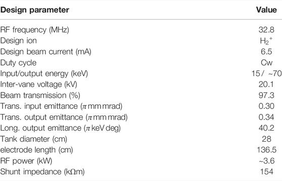
TABLE 1. Basic parameters of the IsoDAR-RFQ, corresponding to the previously developed baseline beam dynamics design and the preliminary RF/mechanical design.
1.2 The Structure of This Paper
We have structured this manuscript into Methodology, Results, and Discussion. In each section, we describe our work separately for the two applications of the SM: 1. As Tuning and Commissioning Tool; 2. As Design and Optimization Tool. These are the natural applications due to the immense speedup of SMs compared to high-fidelity Particle-In-Cell (PIC) simulations. We also present results for a very simple system—the FODO cell—as a benchmark and to elucidate the basic principles and challenges. In the Results, we show that the SM performs excellently as a tuning tool, but issues arise when we vary the hardware parameters of the RFQ. In the Discussion we elaborate possible aspects relevant for the surrogate model to under-perform when the beam dynamics is affected by hardware (design parameter) changes, e.g., space charge, number of design variables or neural network topology.
1.2.1 The Surrogate Model as Tuning and Commissioning Tool
The first application we present is using the SM as an on-line feedback tool during the commissioning and running of the RFQ direct injection prototype. We envision the SM to provide valuable assistance for the operator to allow quick or automated adjustment of the RFQ and beamline settings with respect to the input beam properties. To this end, in the final application, we will train the SM using simulated input values like the signal of beam position monitors (BPMs), the beam current (from an AC Current Transformer [20]), and beam size (from a wire probe) before the RFQ and predict the signals from similar devices after the RFQ. To test the idea in this manuscript, we use the Twiss parameters [21] of the beam as input.
1.2.2 The Surrogate Model as Design and Optimization Tool
Finding an optimized beam dynamics design often requires a very large number of simulation iterations. This makes the design procedure of RFQs time consuming, especially when completely new solutions to meet the required beam output quality need to be explored. This is sometimes even the case for comparatively fast executing beam dynamics codes like PARMTEQM [22] or RFQGen [23], but is definitely a problem when very time consuming PIC simulations are used as the basis for optimization. Similar to demonstrated successes with cyclotrons and electron accelerators [11,24], we are investigating the use of SMs to perform multiobjective optimization for the RFQ modulation cell parameters, in order to yield minimum beam output emittances (transverse and longitudinal) and maximum transmission.
2 Methodology
2.1 Surrogate Modelling
Surrogate models are cheap alternatives to reduce the computational complexity of multiobjective optimizations as already shown in the context of particle accelerators in [25]. We chose neural networks and polynomial chaos expansions to replace the high-fidelity RFQ model codes. These methods are explained in the following subsections. More detailed introductions can be found in the listed references and the references contained therein.
2.1.1 Polynomial Chaos Expansion
The principle of the polynomial chaos expansion (PCE) relies on the orthogonality of the multivariate polynomials Ψi. The high-fidelity model m(x) with input vector
where
is the total number of monomials determined by the expansion truncation order p and the dimensionality of the system d. The vector ξ = (ξ1, … , ξd) represents the input vector that is mapped onto the support of the univariate polynomials ψj. The type of the univariate polynomials of the jth dimension depends on the distribution of the corresponding input dimension. For example, uniformly distributed dimensions are approximated by Legendre polynomials and normally distributed dimensions by Hermite polynomials.
There are multiple methods to obtain the expansion coefficients ci with different requirements on the number of training points N. Commonly used methods are orthogonal projection, regression and Bayesian. In the case of the projection method, the number of training points grows exponentially with the dimension, i.e.,
Regression and Bayesian approaches have no strict requirements, but according to [26] an optimal number of samples is given by
A benefit of PCE based surrogate models is the evaluation of Sobol’ indices [26], a measure of global sensitivity of the output on the input. The first-order Sobol’ index, also known as main sensitivity, quantifies the effect of a single input dimension. The total effect of an input dimension, that also includes all correlations with other dimensions, is denoted as total sensitivity.
We also refer the interested reader to the following literature [26] (and the references therein). Many PCE literature references can also be found in the bibliography of [27].
2.1.2 Artificial Neural Networks
The term “Artificial Neural Network” (ANN) refers to a broad class of methods within Machine Learning (ML) that share the common property of consisting of many interconnected processing units that are used to transform data. The first of such a hierarchy of layers, consists of an affine linear function
The activation function is applied in an element-wise manner, hence a vector activation function σ: Rn → Rn can be defined. Now we are able to define a continuous function f(x) by a composition of linear transforms Ti and activation functions σ, i.e.,
with Ti(x) = Wix + bi. Wi are initially undetermined matrices and bi initially undetermined vectors and σ(⋅) is the element-wise activation function. The values of Wi and bi are randomly initialized and adjusted during “training” using an optimization algorithm to maximize some performance metric.
Such an ANN is called a (k + 1)-layer ANN, which has k hidden layers. Denoting all the undetermined coefficients (e.g., Wi and bi) in Eq. 5 as θ ∈ Θ, where θ is a high dimensional vector and Θ is the span of θ, the ANN representation of a continuous function can now be viewed as
Let
Approximation properties of neural network can be found in [28], [29], where the authors studied approximation properties for the function classes given by a feed-forward neural network with a single hidden layer. In later works, authors studied the error estimates for such neural networks in terms of hyper-parameters such as number of neurons, layers of the network, and activation functions, a review can be found in [30] and [31].
2.2 Data Generation for Surrogate Modelling
The beam dynamics properties of an RFQ with a number of n modulation cells are fully described by the parameter sets B = (B1, ‥, Bn), m = (m1, ‥, mn) and ϕs = (ϕs,1, ‥, ϕs,n), quantifying the basic functions of an RFQ as explained in the sequel:
• The transversely defocusing effect of the space charge force has a 1/γ2-dependency (γ being the Lorentz factor) and hence at low beam velocities efficient and velocity-independent transverse focusing is required. As shown in Figure 1, the alternating electric quadrupole field between the RFQ electrodes leads to a focusing force along one of the transverse axes while defocusing occurs in the perpendicular direction, effectively constituting an alternating gradient focusing channel. The transverse focusing strength in an RFQ cell n is commonly characterized by the parameter Bn [32].
• By adding a sinusoidal modulation to the electrode shape, a longitudinal field component is generated which can be used to adiabatically bunch the DC input beam. This is a highly delicate procedure due to the high sensitivity of space-charge dominated beams to perturbations of the beam particle density. The consecutive modulation cells form a π-mode accelerator structure with a cell length of ℓc = βcλRF/2. The extent of electrode modulation (corresponding to the magnitude of the longitudinal field component) of a cell n is parameterized by the modulation factor mn.
• The synchronous phase ϕs,n, which is set by the cell lengths, determines the ratio of longitudinal bunching to acceleration and hence the overall phase space stability. By increasing ϕs,n along the RFQ, beam acceleration is gradually introduced.

FIGURE 1. Transverse electric quadrupole field around the beam axis of an RFQ (A) with focusing/defocusing plane (green/red) and electrode cell modulation (B), resulting in a longitudinal field component.
Ultimately, the beam output properties depend on the RFQ hardware specifications as well as on the given input beam parameters, which for a DC input beam are specified by the transverse emittances, the Twiss parameters and the beam current.
2.2.1 Simulated Data for a Fixed Radiofrequency Quadrupole Design
To investigate the capability of surrogate models to reproduce the RFQ beam output properties as a function of only the adjustable beam input parameters (in our case the Twiss parameters α and β), we used a fixed preliminary optimized RFQ design, through which we simulated the beam using the PARMTEQM code. A sample data set was obtained from the output of a number of PARMTEQM simulations with randomized values for the input Twiss parameters (corresponding to the design variables of the underlying optimization problem) within a predefined range of α = [1, 4] and β = [7, 25] (cm/mrad). The transverse and longitudinal output emittances as well as the transmission (constituting the optimization objectives) were evaluated directly at the end of the RFQ electrodes.
2.2.2 Simulations of Full Radiofrequency Quadrupole Design
To study the applicability of surrogate models for optimizing the RFQ design itself, we introduced a parameterization of the functions for transverse focusing B(z), synchronous phase ϕ(z) and electrode modulation m(z) according to Figure 2. This reduces the size of the RFQ design parameter space, corresponding to the number of design variables, from 3n + 1 (Bn, ϕs,n, mn for each cell n, + 1 because the number of cells is a design variable itself) to a total number of 14.

FIGURE 2. Parametrization functions for the RFQ cell properties specified by design variables (DVARs): The transversal focusing parameter B(z) is kept constant behind the Radial Matching Section (RMS), with DVAR1 determining the absolute value. Regarding the synchronous phase ϕ(z) and the electrode modulation m(z), the RFQ is subdivided into three sections (slow linear shaping, exponential shaping and exponential bunching), the lengths of which are defined by DVARs 2 and 3. The total slope and the smoothness of the occurrence of the shaping/bunching effect are characterized by DVARs 4–13. Qualitatively, this overall design approach corresponds to a previously developed beam dynamics design using the PARMTEQM RFQ design tools and additionally applying manual changes to the design functions.
The parameterization functions were chosen so that the crucial properties of the underlying baseline design remain variable for optimization; e.g. the constant value of B(z) behind the Radial Matching Section (RMS) (corresponding to DVAR1), the lenghts of the linear and exponential shaping and bunching sections (DVAR2 and DVAR3) as well as the rate and smoothness of shaping and bunching (DVARs 5–13). The length of the RFQ is determined by DVAR14, being the cutoff energy after which PARMTEQM ends the electrode (always with a full RFQ cell).
We generated a sample data set from beam dynamics simulations using PARMTEQM for a number of random RFQ design variations (randomized DVAR values within a predefined range) with a fixed input beam (input Twiss parameters held constant).
2.3 Machine Learning Training and Use of Radiofrequency Quadrupole Surrogate Models
As being best practice for the training of ML models, we randomly split sample datasets into 70% training and 30% test data. A total of 1,000 samples was used for the input beam tuning studies, whereas for the full RFQ optimization with an increased number of design variables, up to 200,000 samples were used. The training data is then used to train either a PCE or NN based surrogate model. After training of the SM, the model predictions are evaluated on both the test and training data by comparison to the original simulation output values. The normalized Mean Absolute Error (MAE) is calculated and reported. To prevent overfitting, the PCE is run repeatedly with increased order to minimize the MAE until the difference between the test and training dataset are more than 5%. In our case, this was at 4th order. A general workflow scheme for surrogate model creation from simulation data is depicted in Figure 3.
To design and train neural networks we used the TensorFlow [33] machine learning framework and the hyperparameter optimization tools provided by Keras [34]. These support automated tuning of the neural network hyperparameters, the used boundary values of which are given in Table 2. We underwent a new hyperparameter scan for each case, and automatically selected the best hyperparameter configuration with minimized MAE for the training set. The choice of a Relu (Rectified Linear Unit) activation function was found to be the best option for the considered use cases. Eventually, the obtained surrogate model can be saved and used for beam dynamics sensitivity studies and optimization.
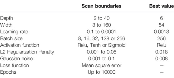
TABLE 2. Hyperparameter boundaries for neural network hyperparameter scan and the best determined value for each case.
Based on the surrogate model, an optimization of the design variables with respect to the objectives using a generic optimizer algorithm can be performed, the result of which (SM output for the best found set of DVARs) can then be validated by the result of the corresponding PARMTEQM beam dynamics simulation output.
3 Results
3.1 Basic FODO Cell Example
The effects of a quadrupole magnet on an ion beam causes focusing on one transverse spatial axis, while leading to defocusing in the perpendicular direction. However, using alternating quadrupoles in series can lead to a net focusing effect for the beam. In accelerator physics, one of the most basic examples of this is called a FODO cell, thus named for focusing (F), drift (0), defocusing (D), and again drift (0). This is schematically depicted in Figure 4.
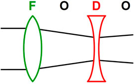
FIGURE 4. Schematic depiction of a FODO cell, showing a transverse projection of the beam envelope undergoing focusing (F), drift (O), defocusing (D) and drift (O).
In order to demonstrate the feasibility of using machine learning techniques to replicate accelerators, we started by reproducing the beam dynamics of this focusing/defocusing FODO lattice. This is the simplest and most basic example that still features similar transverse beam behavior as in RFQs but with greatly reduced overall complexity, and was therefore decided to be a good case to prove the proposed modelling concept.We computed the FODO cell simulations in OPAL [33], using beam input parameters as summarized in Table 3. As shown in Table 6, the generated surrogate model of the FODO cell is capable of mapping the beam input parameters accurately to the values of the output emittances (both transversely and longitudinally) with MAEs of less than 1%, regarding the test data set.
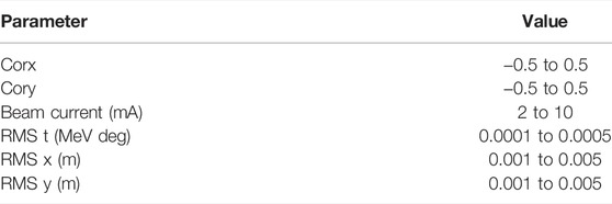
TABLE 3. Input beam design variables to the fixed FODO cell lattice generated using OPAL, and the range of their parameter space.
3.2 FODO Lattice With Varying Cell Parameters
In addition to manipulating the beam input properties and simulating the beam through a fixed FODO cell, we also investigated the case of a variable hardware setup by using the focusing strengths K1 and K2 of the FODO cell quadrupole magnets as design variables. A summary of all design variables of the investigated system is given in Table 4.
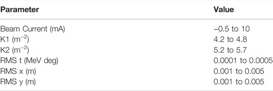
TABLE 4. Design variables and range of their parameter space for the FODO lattice system with varying beam and cell parameters.
This scenario resulted in significantly larger errors compared to the fixed cell example where variation was restricted to the input beam properties. A more detailed discussion of this issue is given later in the discussion section of this paper. The yielded MAE values can again be found in Table 6.
3.3 Creating a Beam Dynamics Tuning Tool for an Radiofrequency Quadrupole
Next, we created a surrogate model with the aim to reproduce the beam dynamics behavior through the RFQ, given a fixed RFQ and variable LEBT input parameters. As summarized in Table 6, a very high model accuracy could be achieved (using either PCE or NN) with values of the normalized MAEs typically being below 1%, regarding transmission and emittances. Corresponding accuracy plots are shown in Figure 5.
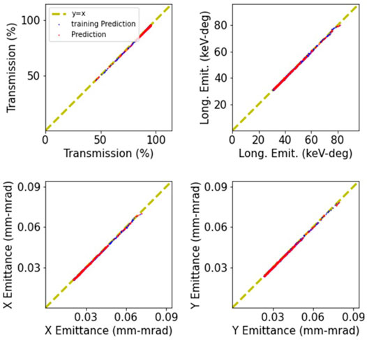
FIGURE 5. Predictions by the neural network surrogate model as function of the actual data values for variation of only the beam input Twiss parameters to a fixed RFQ (MAEs being well below 1%). The red dots correspond to the test dataset whereas the blue dots are training data.
Because executing the surrogate models takes only about 7 ⋅ 10–4 s, given the used computer hardware and software specification, this method can be used to rapidly model the RFQ output for different inputs from the LEBT, allowing to compare simulations and commissioning data in real time. We have thus been able to create a real time, accurate tool for use during the commissioning phase of our RFQ.
Furthermore, we were able to use the same surrogate model to optimize the input beam Twiss parameters (α and β) given a fixed RFQ setup.
Due to the high-fidelity of the achieved surrogate model, the intended optimization of the input beam Twiss parameters for RFQ injection could be performed using a Bayesian optimizer [35], with the SM as the test function and maximum output transmission and minimum output emittances as optimization objectives.
To cross check the optimization results based on the SM, the found optimum set of Twiss parameters was used to validate the predicted SM output by PARMTEQM simulations. The optimum Twiss parameters found for a preliminary revised design of the IsoDAR RFQ are given in Table 5 together with the predicted beam output parameters by the SM and the corresponding PARMTEQM output. Deviations between the simulation and the SM prediction, i.e., optimization result, are less than 0.2% for both transmission and emittance values.
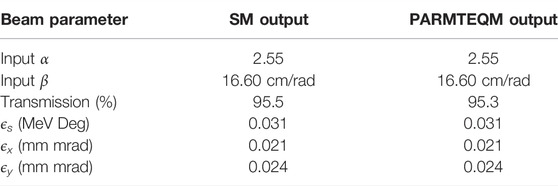
TABLE 5. Optimum set of Twiss parameters found by Bayesian optimizer based on the surrogate model output and corresponding predicted beam output parameters with comparison to PARMTEQM results.
3.4 Optimization of the Entire Radiofrequency Quadrupole Beam Dynamics Design on the Basis of Surrogate Models
Ultimately, we used the 14-DVAR RFQ model sample data set to train PCE and NN based models. Corresponding accuracy plots can be seen in Figure 6 and achieved MAEs are again summarized in Table 6.Similar to the previous case, the obtained surrogate models execute much faster than their simulation counterparts. Whereas the calculation of a SM prediction takes around 10−3 s, a corresponding physics beam dynamics simulation with PARMTEQM of a short IsoDAR type RFQ with an electrode length of around 1.3 m consumes up to around 40 s. With a sufficiently large design space, this significantly reduces the time to find an optimized RFQ beam dynamics design.
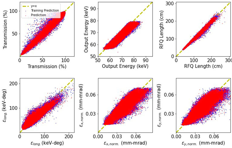
FIGURE 6. Surrogate model predictions as function of the actual data values for full RFQ design variation by 14 DVARs and fixed beam input Twiss parameters. Again, the red dots correspond to the test dataset and the blue dots are training data.

TABLE 6. Comparison between mean average errors (MAEs) for surrogate models based on polynomial chaos expansion (PCE) and neural networks (NN) for different optimization cases and objectives.
With MAEs of the predicted output emittances of up to 10% (the MAEs for the transmission however being noticeably smaller) we found the surrogate models currently do not provide decent enough accuracy in any of the considered cases to perform a full RFQ design optimization. However, these computationally inexpensive surrogate models can be used to perform a rough pre-optimization with respect to the beam output objectives, providing a starting point for fine tuning optimizations using beam dynamics simulation tools. Using these methods combined reduces the total computational need of RFQ optimization and allows to quickly explore different possible qualitative solution approaches.
4 Discussion
The created surrogate models quickly proved to be a reliable rapid-use tool for observing the effects of input beam variations on the output beam properties of a given RFQ. This has been a useful tool in optimizing the LEBT design, and could be as much as useful during commissioning and tuning of the LEBT/RFQ system. Ultimately, we found that highly accurate (
On the other hand, however, the application of the developed techniques to the full RFQ beam dynamics design optimization proved problematic due to increased errors in predicted emittance whenever the space of design variables was expanded to include physical changes to the RFQ. This problem also already occurred in the case of the FODO cell. As shown in Figure 6 and summarized in Table 6, models that include structural changes of the accelerator hardware system, such as variation of the FODO cell focusing strengths and the full RFQ optimization, suffer from errors in the emittances prediction
As depicted in Figure 7, the surrogate model lends itself to perform sensitivity analyses investigating the impact of DVAR variation on the optimization objectives.
Eventually, this allows for an evaluation of the cell properties parameterization model and to reduce the number of DVARs by omitting design variables with little effect on the crucial optimization objectives.
In case of our specific RFQ, the sensitivity chart (Figure 7) reaveals that variation of DVARs 9, 10 and 13 (all relating to the function ϕ(z) of the synchronous phase) have the most significant influence on the transverse emittances, while the longitudinal emittance seems to be most sensitive to DVAR5 (value of the modulation factor m(z) at the end of the exponential shaping section). Potential DVAR variations that might be omitted for the optimization procedure apparently relate to DVAR1 (value of the transverse focusing parameter B(z) = const.) and DVARs 2 and 4 (properties of m(z) in the slow linear shaping section) as well as DVARs 3 and 6 (properties of m(z) in the exponential shaping section).
5 Conclusion
In this paper, we applied a recently developed surrogate modelling technique to the optimization of the beam output quality of RFQ linear accelerators for the first time. We tested our method on a simple FODO cell (having similar transverse focusing properties) first and on the IsoDAR RFQ thereafter. To create the surrogate models, we used polynomial chaos expansion and deep neural networks. We compared the results and found that we could very accurately predict the beam behaviour from varying input beam parameters as it goes through a fixed accelerator structure, which initially was our main goal. The trained model is intended to be used as an online feedback tool in the commissioning and tuning of the IsoDAR injector. Furthermore, we found that, when we train the surrogate model on sets of hardware parameters (i.e., many different design configurations of the investigated machine), we incur much higher training and validation errors. We are in the process of investigating the cause of this effect, and we can already say that, in a comparison between beams with and without space charge, we do not see a difference. Despite the large training errors (up to 10%), the surrogate models trained on hardware design variables can be used to perform preliminary optimization of the design, reducing the model space, followed by a second iteration using high-fidelity physics simulations. Furthermore, Sobol’s indices can be used to elucidate the influence of single design variables on the objectives, allowing restricting design variations to the most crucial parameters.
Data Availability Statement
The raw data supporting the conclusion of this article will be made available by the authors, without undue reservation.
Author Contributions
DK, DW, and LW contributed to conception and design of the study. DK conducted all RFQ beam dynamics studies. LW performed the machine learning studies. DW and JC supervised the project. AA and MF provided the Jupyter notebooks (PCE scripts and NN topology) for the machine learning studies and provided support on all machine learning problems, and also provided the OPAL simulations. DK, LW, and DW wrote the first draft of the manuscript and MF wrote the theory section. All authors contributed to manuscript revision, read, and approved the submitted version.
Funding
This work was supported by NSF grants PHY-1505858 and PHY-1626069 and funding from the Bose Foundation and the Heising-Simons Foundation.
Conflict of Interest
The authors declare that the research was conducted in the absence of any commercial or financial relationships that could be construed as a potential conflict of interest.
Publisher’s Note
All claims expressed in this article are solely those of the authors and do not necessarily represent those of their affiliated organizations, or those of the publisher, the editors and the reviewers. Any product that may be evaluated in this article, or claim that may be made by its manufacturer, is not guaranteed or endorsed by the publisher.
References
1. Ren S, He K, Girshick R, Sun J. Faster R-Cnn: Towards Real-Time Object Detection with Region Proposal Networks. In: C Cortes, N Lawrence, D Lee, M Sugiyama, and R Garnett, editors. Advances in Neural Information Processing Systems, 28. Curran Associates, Inc. (2015).
2. He K, Zhang X, Ren S, Sun J. Deep Residual Learning for Image Recognition. In: IEEE Conference on Computer Vision and Pattern Recognition (CVPR) (2016). 770–8. doi:10.1109/CVPR.2016.90
3. Abadi M, Agarwal A, Barham P, Brevdo E, Chen Z, Citro C, et al. TensorFlow: Large-Scale Machine Learning on Heterogeneous Systems (2015). Software available from tensorflow.org [Dataset].
5. Ren X, Edelen A, Lutman A, Marcus G, Maxwell T, Ratner D, Temporal Power Reconstruction for an X-ray Free-Electron Laser Using Convolutional Neural Networks. Phys Rev Acc Beams. 23 (2020). American Physical Society. 040701. doi:10.1103/PhysRevAccelBeams.23.040701.Publisher
6. Kirschner J, Mutny M, Hiller N, Ischebeck R, Krause A. Adaptive and Safe Bayesian Optimization in High Dimensions via One-Dimensional Subspaces (2019). arXiv:1902.03229 [cs, stat] ArXiv: 1902.03229.
7. Kirschner J, Nonnenmacher M, Mutny M, Krause A, Hiller N, Ischebeck R, et al. Bayesian Optimisation for Fast and Safe Parameter Tuning of SwissFEL. JACoW Publishing (2019). p. 707–10. doi:10.3929/ethz-b-000385955
8. Duris J, Kennedy D, Hanuka A, Shtalenkova J, Edelen A, Baxevanis P, et al. Bayesian Optimization of a Free-Electron Laser. Phys Rev Lett (2020) 124:124801. American Physical Society. doi:10.1103/PhysRevLett.124.124801.Publisher
9. Adelmann A. On Nonintrusive Uncertainty Quantification and Surrogate Model Construction in Particle Accelerator Modeling. Siam/asa J Uncertainty Quantification (2019) 7:383–416. doi:10.1137/16M1061928
10. Van Der Veken F, Azzopardi G, Blanc F, Coyle L, Fol E, Giovannozzi M, et al. Machine Learning in Accelerator Physics: Applications at the CERN Large Hadron Collider. SISSA Medialab (2020) 372:044. doi:10.22323/1.372.0044
11. Edelen AL, Biedron SG, Milton SV, Edelen JP. First Steps toward Incorporating Image Based Diagnostics into Particle Accelerator Control Systems Using Convolutional Neural Networks (2016). arXiv:1612.05662 [physics] ArXiv: 1612.05662.
12. Edelen A, Neveu N, Frey M, Huber Y, Mayes C, Adelmann A. Machine Learning for Orders of Magnitude Speedup in Multiobjective Optimization of Particle Accelerator Systems. Phys Rev Accel Beams (2020) 23:044601. doi:10.1103/PhysRevAccelBeams.23.044601
13. Bungau A, Adelmann A, Alonso JR, Barletta W, Barlow R, Bartoszek L, 109. American Physical Society (2012). p. 141802. doi:10.1103/PhysRevLett.109.141802.PublisherProposal for an Electron Antineutrino Disappearance Search Using High-Rate $ˆ\\{8\\}∖mathrm\\{Li\\}$ Production and DecayPhys Rev Lett
14. Abs M, Adelmann A, Alonso JR, Axani S, Barletta WA, Barlow R, et al. IsoDAR@KamLAND: A Conceptual Design Report for the Technical Facility (2015). arXiv:1511.05130 [hep-ex, physics:physics] ArXiv: 1511.05130.
15. Winklehner D, Bahng J, Calabretta L, Calanna A, Chakrabarti A, Conrad J, et al. enHigh Intensity Cyclotrons for Neutrino Physics. Nucl Instr Methods Phys Res Section A: Acc Spectrometers, Detectors Associated Equipment (2018) 907:231–43. doi:10.1016/j.nima.2018.07.036
16. Diaz A, Argüelles CA, Collin GH, Conrad JM, Shaevitz MH. Where Are We with Light Sterile Neutrinos (2019). arXiv:1906.00045 [hep-ex, physics:hep-ph] ArXiv: 1906.00045.
17. Calanna A, Campo D, Yang JJ, Calabretta L, Rifuggiato D, Maggiore MM, et al. A Compact High Intensity Cyclotron Injector for DAEdALUS Experiment, C1205201 (2012). p. 424–6.
18. Winklehner D, Adelmann A, Conrad JM, Mayani S, Muralikrishnan S, Schoen D, et al. Order of Magnitude Beam Current Improvement in Compact Cyclotrons (2021). arXiv:2103.09352 [physics].
19. Winklehner D, Hamm R, Alonso J, Conrad J. An RFQ Direct Injection Scheme for the IsoDAR High Intensity Cyclotron $\\mathrm{H}_{2}^+$. In: 6th International Particle Accelerator Conference (2015). IPAC2015).
20. Bergoz . Bergoz - ACCT - Precise Waveform Measurement of Long Pulses (2020). [Dataset] Available at: https://www.bergoz.com/products/acct/.
22. Crandall KR, Wangler TP, 177. PARMTEQ €” A Beam-Dynamics Code Fo the RFQ Linear Accelerator. Linear Accelerator Beam Opt Codes (1988). AIP Publishing. 22–8.
24. Neveu N, Spentzouris L, Adelmann A, Ineichen Y, Kolano A, Metzger-Kraus C, et al. Parallel General Purpose Multiobjective Optimization Framework with Application to Electron Beam Dynamics. Phys Rev Accel Beams (2019) 22:054602. doi:10.1103/PhysRevAccelBeams.22.054602
25. Sudret B. Global Sensitivity Analysis Using Polynomial Chaos Expansions. Reliability Eng Syst Saf (2008) 93:964–79. doi:10.1016/j.ress.2007.04.002
26. Sobol’ IM. Global Sensitivity Indices for Nonlinear Mathematical Models and Their Monte Carlo Estimates. Mathematics Comput Simulation (2001) 55:271–80. doi:10.1016/S0378-4754(00)00270-6
27. Frey M, Adelmann A. Global Sensitivity Analysis on Numerical Solver Parameters of Particle-In-Cell Models in Particle Accelerator Systems. Comp Phys Commun (2021) 258:107577. doi:10.1016/j.cpc.2020.107577
28. Cybenko G. Approximation by Superpositions of a Sigmoidal Function. Maths Control Signals Syst (1989) 2:303–14. doi:10.1007/bf02551274
29. Hornik K, Stinchcombe M, White H. Multilayer Feedforward Networks Are Universal Approximators. Neural Networks (1989) 2:359–66. doi:10.1016/0893-6080(89)90020-8
30. Ellacott SW. Techniques for the Mathematical Analysis of Neural Networks. J Comput Appl Math (1994) 50:283–97. doi:10.1016/0377-0427(94)90307-7
31. Pinkus A. Approximation Theory of the Mlp Model in Neural Networks. Acta Numerica (1999) 8:143–95. doi:10.1017/S096249290000291910.1017/s0962492900002919
32. Crandall K, Stokes R, Wangler T. RF Quadrupole Beam Dynamics Design Studies. In: Proceedings of LINAC1979 (1979).
33. Adelmann A, Gsell A, Kraus C, Ineichen Y, Russell S, Bi Y, et al. The OPAL (Object Oriented Parallel Accelerator Library) Framework. Tech. Rep. PSI-PR-08-02, Paul Scherrer Institut (2008). 2015.
34. Nogueira F. Bayesian Optimization: Open Source Constrained Global Optimization Tool for Python[Dataset] (2014).
Keywords: radio frequency quadrupole, beam dynamics design, beam matching, virtual accelerator, isodar, surrogate modelling, neural network, polynomial chaos expansion
Citation: Koser D, Waites L, Winklehner D, Frey M, Adelmann A and Conrad J (2022) Input Beam Matching and Beam Dynamics Design Optimizations of the IsoDAR RFQ Using Statistical and Machine Learning Techniques. Front. Phys. 10:875889. doi: 10.3389/fphy.2022.875889
Received: 14 February 2022; Accepted: 22 March 2022;
Published: 25 April 2022.
Edited by:
Frank Franz Deppisch, University College London, United KingdomReviewed by:
Gianluca Valentino, University of Malta, MaltaBaoxi Han, Oak Ridge National Laboratory (DOE), United States
Copyright © 2022 Koser, Waites, Winklehner, Frey, Adelmann and Conrad. This is an open-access article distributed under the terms of the Creative Commons Attribution License (CC BY). The use, distribution or reproduction in other forums is permitted, provided the original author(s) and the copyright owner(s) are credited and that the original publication in this journal is cited, in accordance with accepted academic practice. No use, distribution or reproduction is permitted which does not comply with these terms.
*Correspondence: Daniel Koser, ZGtvc2VyQG1pdC5lZHU=
 Daniel Koser
 Loyd Waites1
 Daniel Winklehner
 Andreas Adelmann
