 Tomás Chacón Rebollo
 Macarena Gómez Mármol2
- 1Departamento EDAN & IMUS, Universidad de Sevilla, Sevilla, Spain
- 2Departamento EDAN, Universidad de Sevilla, Sevilla, Spain
- 3Departamento Matemática Aplicada I, Universidad de Sevilla, Sevilla, Spain
In this study, we obtained low-rank approximations for the solution of parametric non-symmetric elliptic partial differential equations. We proved the existence of optimal approximation subspaces that minimize the error between the solution and an approximation on this subspace, with respect to the mean parametric quadratic norm associated with any preset norm in the space of solutions. Using a low-rank tensorized decomposition, we built an expansion of approximating solutions with summands on finite-dimensional optimal subspaces and proved the strong convergence of the truncated expansion. For rank-one approximations, similar to the PGD expansion, we proved the linear convergence of the power iteration method to compute the modes of the series for data small enough. We presented some numerical results in good agreement with this theoretical analysis.
1 Introduction
This study deals with the low-rank tensorized decomposition (LRTD) of parametric non-symmetric linear elliptic problems. The basic objective in model reduction is to approximate large-scale parametric systems by low-dimension systems, which are able to accurately reproduce the behavior of the original systems. This allows tackling in affordable computing times, control, optimization, and uncertainty quantification problems related to the systems modeled, among other problems requiring multiple computations of the system response.
The PGD method, introduced by Ladévèze in the framework of the LATIN method (LArge Time INcrement method [22]) and extended to multidimensional problems by Ammar et al [2], has experienced an impressive development with extensive applications in engineering problems. This method is an a priori model reduction technique that provides a separate approximation of the solution of parametric PDEs. A compilation of advances in the PGD method may be found in [11].
Among the literature studying the convergence and numerical properties of the PGD, we can highlight [1], where the convergence of the PGD for linear systems of finite dimension is proved. In [8], the convergence of the PGD algorithm applied to the Laplace problem is proven, in a tensorized framework. The study [9] proves the convergence of the PGD for an optimization problem, where the functional framework is strongly convex and has a Lipschitz gradient in bounded sets. In [17], the authors prove the convergence of an algorithm similar to a PGD for the resolution of an optimization problem for a convex functional defined on a reflective Banach space. In [16], the authors prove the convergence of the PGD for multidimensional elliptic PDEs. The convergence is achieved because of the generalization of Eckart and Young’s theorem.
The present study is motivated by [5], where the authors present and analyze a generalization of the previous study [16] when operator A depends on a parameter. The least-squares LRTD is introduced to solve parametric symmetric elliptic equations. The modes of the expansion are characterized in terms of optimal subspaces of a finite dimension that minimize the residual in the mean quadratic norm generated by the parametric elliptic operator. As a by-product, this study proves the strong convergence in the natural mean quadratic norm of the PGD expansion.
A review of low-rank approximation methods (including PGD) may be found in the studies [18, 19]. In particular, minimal residual formulations with a freely chosen norm for Petrov–Galerkin approximations are presented. In addition, the study [10] gives an overview of numerical methods based on the greedy iterative approach for non-symmetric linear problems.
In [3, 4], a numerical analysis of the computation of modes for the PGD to parametric symmetric elliptic problems is reported. The nonlinear coupled system satisfied by the PGD modes is solved by the power iteration (PI) algorithm, with normalization. This method is proved to be linearly convergent, and several numerical tests in good agreement with the theoretical expectations are presented.
Actually, for symmetric problems, the PI algorithm to solve the PGD modes turns out to be the adaptation of the alternating least-squares (ALS) method thoroughly used to compute tensorized low-order approximations of high-order tensors. The ALS method was used in the late 20th century within the principal components analysis (see [6, 7, 20, 21]) and extended in [27] to the LRTD approximation of high-order tensors. Its convergence properties were subsequently analyzed by several authors; local and global convergence proofs within several approximation frameworks are given in [14, 25, 26]. Several generalizations were reported; as mentioned, without intending to be exhaustive, in the studies [12–15, 23].
The convergence proofs within the studies [14, 25, 26] cannot be applied to our context as we are dealing with least-squares with respect to the parametric norm intrinsic to the elliptic operator, even for symmetric problems. Comparatively, the difference is similar to that between proving the convergence of POD or PGD approximations to elliptic PDEs. The POD spaces are optimal with respect to a user-given fixed norm, while the PGD spaces are optimal with respect to the intrinsic norm associated to the elliptic operator (see [5]). This use of the intrinsic parametric norm does not make it necessary the previous knowledge of the tensor object to be approximated (in our study, the parametric solution of the targeted PDE), as is needed in standard ALS algorithms.
In the present study, we propose an LRTD to approximate the solution of parametric non-symmetric elliptic problems based upon symmetrization of the problem (Section 2). Each mode of the series is characterized in terms of optimal subspaces of finite dimension that minimize the error between the parametric solution and its approximation on this subspace, but now with respect to a preset mean quadratic norm as the mean quadratic norm associated to the operator in the non-symmetric case is not well-defined (Section 3). We prove that the truncated LRTD expansion strongly converges to the parametric solution in the mean quadratic norm (Section 4).
The minimization problems to compute the rank-one optimal modes are solved by a PI algorithm (Section 5). We prove that this method is locally linearly convergent and identifies an optimal symmetrization that provides the best convergence rates of the PI algorithm, with respect to any preset mean quadratic norm (Section 6).
We finally report some numerical tests for 1D convection–diffusion problems that confirm the theoretical results on the convergence of the LRTD expansion and the convergence of the PI algorithm. Moreover, the computing times required by the optimal symmetrization are compared advantageously to those required by the PGD expansion (Section 7).
2 Parametric Non-Symmetric Elliptic Problems
Let us consider the mathematical formulation for parametric elliptic problems introduced in [5] that we shall extend to non-symmetric problems.
Let
where
It is assumed that a (⋅, ⋅; γ) is uniformly continuous and uniformly coercive on H μ-a. e. γ ∈ Γ and there exist positive constants α and β independent of γ such that,
By the Lax–Milgram theorem, problem (1) admits a unique solution μ-a. e. γ ∈ Γ. To treat the measurability of u with respect to γ, let us consider the problem:
Let f be a function that belongs to
where
By the Lax–Milgram theorem, owing to (2) and (3), problem (4) admits a unique solution. Problems (1) and (4) are equivalent in the sense that (see [5])
We shall consider a symmetrized reformulation of the formulation (4). Let us consider a family of inner products in H,
considering the associated scalar product in
Let us define a new bilinear form
It is to be noted that
Thus, as a consequence of (2) and (3), the form
Now, problem (4) is equivalent to
We shall use this formulation to build optimal approximations of problem (1) on subspaces of finite-dimension, when the form
where u is the solution of problem (4) and uZ is its approximation given by the Galerkin approximation of problem (10) in
Then, for any
Theorem 2.1 For any k ≥ 1, problem (11) admits at least one solution.
3 Targeted-Norm Optimal Subspaces
It is assumed that we give a family of inner products
In this way, the optimal subspaces are the solution of the problem
Let us consider the operators Aγ,⋆: H↦H and the bilinear forms (⋅,⋅)γ,⋆ on H × H defined by
It is to be noted that Aγ,⋆ is an isomorphism on H and consequently (⋅,⋅)γ,⋆ is an inner product on H. Due to (2) and (3), the norms generated by these inner products are uniformly equivalent to the reference norm in H. Moreover, by (14) and (15),
Let us consider now the inner product in
Then, it holds.
Lemma 1 Let Aγ : H → H be the continuous linear operators defined by
Then, it holds
This result follows from a standard argument using the separability of space H that we omit for brevity. Then, by Lemma 1, we have
Let us denote by
As a consequence, the optimal subspaces obtained by the least-squares problem (11) when
Remark 1 When the forms a (⋅, ⋅; γ) are symmetric, if we choose
then Aγ,⋆ defined by (14) is the identity operator in H. From (21), it follows that
4 A Deflation Algorithm to Approximate the Solution
Following the PGD procedure, we approximate the solution of problem (1) by a tensorized expansion with summands of rank
computed by the following algorithm:
Initialization: let be u0 = 0.
Iteration: assuming ui−1, known for any i ≥ 1, set ei−1≔u − ui−1. Then,
with
It is to be noted that this algorithm does not need to know the solution u of problem (4) since ei−1 is defined in terms of the current residual
The convergence of the uN to u is stated in Theorem 5.3 of [5] as the form
Theorem 4.1 The truncated series uN determined by the deflation algorithm (24)–(26) satisfying
Consequently, uN strongly converges in
5 Rank-One Approximations
An interesting case from the application point of view arises when we consider rank-one approximations. Indeed, when k = 1, the solution of (12) uZ can be obtained as
Then, the problem (11) can be written as (see [5], Sect. 6)
where
Any solution of problem (27) has to verify the following conditions:
Proposition 1 If
We omit the proof of this result for brevity; let us just mention that conditions (29) and (30) are the first-order optimality conditions of the problem (27) that take place as the functional
Relations (29)–(30) suggest an alternative way to compute the modes in the PGD expansion to solve (1). Indeed, we propose a LRTD expansion for u given by
where the modes
If this problem is solved in such a way that its solution is also a solution of
then expansion (31) will be optimal in the sense of the expansion (24), where each mode of the series is computed in an optimal finite-dimensional subspace that minimizes the error.
6 Computation of Low-Rank Tensorized Decomposition Modes
In this section, we analyze the solution of the nonlinear problem (32) by the power iteration (PI) method. As the operator Aγ appears in the test functions, a specific treatment is needed, in particular, to compute targeted-norm subspaces. We also introduce a simplified PI algorithm that does not need to compute Aγ. Here, we report both.
We focus on solving the model problem (29)–(30), which we assume to admit a nonzero solution. For simplicity, the notation f will stand either for the r. h. s. of the problem (4) or for any residual fi.
It is to be observed that (30) is equivalent to
and then
Thus, problem (29)–(30) consists in
with
Let us define the operator T : H → H that transforms w ∈ H into T(w) ∈ H solution to the problem
T is well-defined from (2) and (3), and a solution of (35) is a fixed point of this operator. Moreover, as Aγ is linear,
Thus, if (w, φ) is a solution to (29)–(30), then (λ w, λ−1φ) is also a solution to this problem. So, we propose to find a solution to problem (35) with unit norm. For that, we apply the following PI algorithm with normalization:
Initialization:Given any nonzero w0 ∈ H such that φ0 = φ(w0) is not zero in
Iteration: Knowing wn ∈ H, the following is computed :
The next result states that this iterative procedure is well-defined.
Lemma 2 It is assumed that for some nonzero w ∈ H, it holds that
Proof First, by reduction to the absurd, it is assumed that T(w) = 0. From (36), we have
In particular, for v = w and taking into account (34), we deduce that
Then,
and thus, φ(w) = 0 is in contradiction with the initial hypothesis. This proves that T(w) is not zero. Second, arguing again by reduction to the absurd, it is assumed that
Then, setting
As
We have already proven that
This result proves that if w0 and φ0 are not zero, then the algorithm (37) is well-defined.
6.1 Computation of Power Iteration Algorithm for Targeted-Norm Optimal Subspaces
From a practical point of view, in general, the algorithm (37) is computationally expensive. Indeed, in practice, H is a space of large finite-dimension and the integral in Γ is approximated by some quadrature rule with nodes
It is to be noted that when targeted subspaces are searched for, in the way considered in Section 3, the expression of algorithm (37) simplifies. Indeed, as a (w, Aγ,⋆v; γ) = (w,v)H,γ, then
In addition, the problem (36) that defines the operator T simplifies to problem:
We shall refer to the method (38)–(39) as the TN (targeted-norm) method.
6.2 A Simplified Power Iteration Algorithm
An approximate, but less expensive, method is derived from the observation that Aγ is an isomorphism in H. If we approximate the first equation in (32) by
for some γ0 ∈ Γ, then this equation is equivalent to
We then consider the following adaptation of the PI method (37) to compute an approximation of the solution of the optimality conditions (32):
Iteration: Known wn ∈ H, the following is computed:
where
where φ(w, γ) is defined by (34). We shall refer to method (41)–(42) as the STN (simplified targeted-norm) method. The difference between the STN method and the standard PGD one is only the definition of the function φ that in this case is given by
6.3 Convergence of the Power Iteration Algorithms
In this section, we analyze the convergence of the PI algorithms (37) and (41) (Theorem 6.1). We prove that the method with optimal convergence rate corresponds to the operator Aγ,⋆ introduced in Section 3, choosing all the inner products ‖ ⋅‖H,γ equal to the reference inner product ‖ ⋅‖.
As in [5], we shall assume that the iterates φn remain in the exterior of some ball of positive radius, say ɛ > 0, of
This is a working hypothesis that makes sense whenever the mode that we intend to compute is not zero, considering that the wn is normalized.
From the definition of Aγ and (6), it holds
where α and β are given by (2) and (3), respectively, and αH and βH are defined in (6).
Let us define the function:
It holds.
Theorem 6.1 It is assumed that (43) holds, and
Then, there exists a unique solution with norm 1 w of problem (35); the sequence
As a consequence, the sequence
Proof. Let us consider at first the method (37). Let x ∈ BH(w, r) such that
We aim to estimate
It holds
using (44). Thus,
Moreover,
Setting
To bound the second term in the r. h s. of (53), from (34), it holds
where
‖w‖ − r ≤ ‖x‖ and then
where
It is to be noted that from (34),
Hence,
where
Combining (53) with (55) and (57), we deduce
Setting
Thus,
It holds
That is,
Estimate (46) follows from this last inequality for x = wn, assuming that wn ∈ BH(w, r). Assuming w0 ∈ BH(w, r) this recursively proves that all the wn are in BH(w, r). Furthermore, suppose that there exists another solution to (35) with norm one in the ball BH(w, r), w*. In this case, estimating (60) for x = w* implies
because
Let us now consider method (41). In this case
To estimate
As ⟨f(γ), v⟩ = a (u(γ), v; γ) ≤ β ‖u(γ)‖ ‖v‖, ∀ v ∈ H, setting
The functions φ(w) and φ(x) have the same expressions for methods (37) and (41).
Moreover, setting
Hence,
As
Remark 2 The optimal convergence rate Δ corresponds to k = 1 and λ = 1, that is,
Then, from (44), choosing all the inner products ‖ ⋅‖H,γ equal to the reference inner product ‖ ⋅‖, we obtain
Remark 3 If we intend to compute a mode of order i ≥ 2, Theorem 6.1 and Remark 2 also hold, replacing f by the residual
7 Numerical Tests
In this section, we discuss the numerical results obtained with the methods TN (38)–(39) and STN (41)–(42) to solve some non-symmetric second-order PDEs. Our purpose, on the one hand, is to confirm the theoretical results stated in Theorem 4.1 and Theorem 6.1, and on the other hand, to compare the practical performances of these methods with the standard PGD.
We consider a parametric 1D advection–diffusion problem with fixed constant advection velocity β,
We assume that β = 1, and then γ is the Péclet number. The source term is f = 1/500. We have set Γ = [2.5, 50]; then, there is a large asymmetry of the advection–diffusion operator.
Once the nonhomogenous boundary condition at x = 0 is lifted, problem (66) is formulated under the general framework (1) when the space H and the bilinear form a (⋅, ⋅) are given by H = {v ∈ H1(Ω) |v (0) = 0 }, and
We endow space H with the
In practice, we replace the continuous problem (1) by an approximated one on a finite element space Hh formed by piecewise affine elements. In addition, the integrals on Γ are approximated by a quadrature formula constructed on a subdivision of Γ into M subintervals,
This is equivalent to approximating the Lebesgue measure μ by a discrete measure μΔ located at the nodes of the discrete set ΓΔ = {γi, i = 1, … , M} with weights ωi, i = 1, … , M. Consequently, all the theoretical results obtained in the previous sections apply, by replacing the
In our computations, we have used the midpoint quadrature formula with M = 100 equally spaced subintervals of Γ to construct IM and constructed Hh with 300 subintervals of Ω of the same length.
Test 1:
This first experiment is intended to check the theoretical results on the convergence rate of the PI algorithm, stated in Theorem 6.1, for the TN and STN methods: we consider optimal targeted subspaces, in the sense of the standard
to define the mappings Aγ,⋆ by (14) and the form
For each mode wi of the LRTD expansion (31), we have estimated the numerical convergence rate of the PI algorithm by
Tables 1 and 2 show the norm of the difference between two consecutive approximations and the ratios
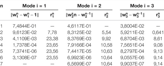
TABLE 1. Convergence rates of the PI algorithm for the first TN modes.
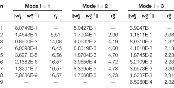
TABLE 2. Convergence rates of the PI algorithm for the first STN modes.
We observe that the PI method converges with a nearly constant rate for each mode, in agreement with Theorem 6.1. The convergence rate is larger for the TN method, also as expected from this theorem. It is also noted that the convergence rates are smaller for higher-order modes.
In Figure 1, we present the comparison between the solution obtained by finite elements for γ = 2.7375 and γ = 49.7625 and the truncated series sum for the TN, the results for the STN are similar.
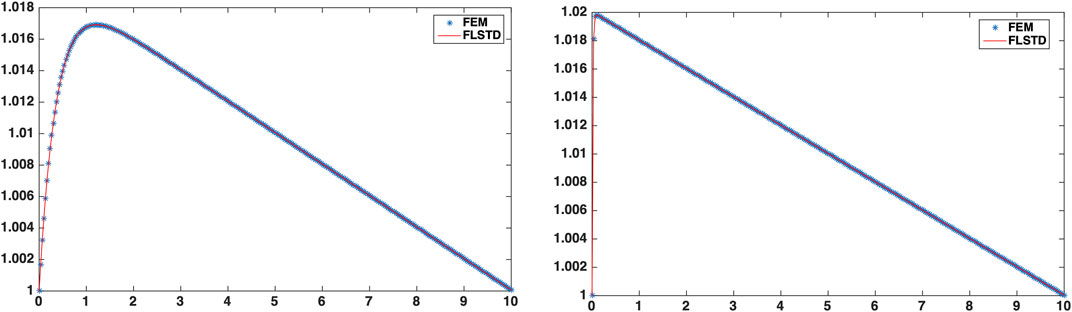
FIGURE 1. Solutions of problem (66) by the LRTD (called FLSTD within the figure) expansion computed with the TN method. Left γ = 2.7375 Right γ = 49.7624.
Test 2:
In this test, we compare the convergence rates of PGD, TN, and STN methods to obtain the LRTD expansion (31) for the problem (66).
Figure 2 displays the errors of the truncated series with respect to the number of modes, in norm
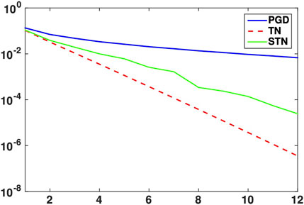
FIGURE 2. Convergence history of the PGD, TN, and STN series for Test 2.
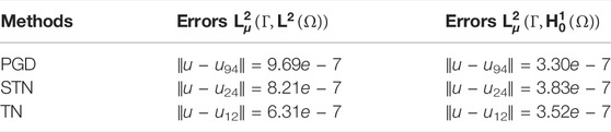
TABLE 3. Numerical behavior of the PGD, STN, and TN methods for Test 2.
Finally, we compare the CPU times required by the three methods. By construction, it is clear that to compute every single iteration of the PI method, the TN method is much more expensive since it involves the calculation of the Aγ,* operator for each finite element base function. However, due to the fast convergence of the associated LRTD expansion, it is less expensive than PGD to compute the expansion. Figure 3 displays the CPU times for the TN, STN, and PGD methods as a function of the number of subintervals M considered in the partition of Γ. The STN method is more expensive than the PGD method; this arises due to the small convergence rate of the PI algorithm with the STN method. However, the TN method is less expensive than the PGD one, requiring approximately half the CPU time.
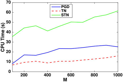
FIGURE 3. Comparison of CPU times to compute the TN, STN, and PGD expansions.
8 Conclusion
In this study, we have proposed a new low-rank tensorized decomposition (LRTD) to approximate the solution of parametric non-symmetric elliptic problems, based on symmetrization of the problem.
Each mode of the series is characterized as a solution to a calculus of variation problem that yields an optimal finite-dimensional subspace, in the sense that it minimizes the error between the parametric solution and its approximation on this subspace, with respect to a preset mean quadratic norm. We have proven that the truncated expansion given by the deflation algorithm strongly converges to the parametric solution in the mean quadratic norm.
The minimization problems to compute the rank-one optimal modes are solved by the power iteration algorithm. We have proven that this method is locally linearly convergent when the initial data are close enough to an optimal mode. We also have identified an optimal symmetrization that provides the best convergence rates of the PI algorithm, with respect to the preset mean quadratic norm.
Furthermore, we have presented some numerical tests for 1D convection–diffusion problems that confirm the theoretical results on the convergence of the LRTD expansion and the convergence of the PI algorithm. Moreover, the computing times required by the optimal symmetrization compare advantageously to those required by the PGD expansion.
In this study, we have focused on rank-one tensorized decompositions. In our forthcoming research, we intend to extend the analysis to ranks k ≥ 2. This requires solving minimization problems on a Grassmann variety to compute the LRTD modes. We will also work on the solution of higher-dimensional non-symmetric elliptic problems by the method introduced in order to reduce the computation times as these increase with the dimension of the approximation spaces.
Data Availability Statement
The original contributions presented in the study are included in the article, further inquiries can be directed to the corresponding author.
Author Contributions
TC and IS performed the theoretical derivations while MG did the computations.
Funding
The research of TC and IS has been partially funded by PROGRAMA OPERATIVO FEDER ANDALUCIA 2014-2020 grant US-1254587, which in addition has covered the cost of this publication. The research of MG is partially funded by the Spanish Research Agency - EU FEDER Fund grant RTI2018-093521-B-C31.
Conflict of Interest
The authors declare that the research was conducted in the absence of any commercial or financial relationships that could be construed as a potential conflict of interest.
Publisher’s Note
All claims expressed in this article are solely those of the authors and do not necessarily represent those of their affiliated organizations, or those of the publisher, the editors, and the reviewers. Any product that may be evaluated in this article, or claim that may be made by its manufacturer, is not guaranteed or endorsed by the publisher.
References
1. Ammar A, Chinesta F, Falcó A. On the Convergence of a Greedy Rank-One Update Algorithm for a Class of Linear Systems. Arch Computat Methods Eng (2010) 17:473–86. Number 4. doi:10.1007/s11831-010-9048-z
2. Ammar A, Mokdad B, Chinesta F, Keunings R. A New Family of Solvers for Some Classes of Multidimensional Partial Differential Equations Encountered in Kinetic Theory Modeling of Complex Fluids. J Non-Newtonian Fluid Mech (2006) 139:153–76. doi:10.1016/j.jnnfm.2006.07.007
3. Azaïez M, Chacón Rebollo T, Gómez Mármol M. On the Computation of Proper Generalized Decomposition Modes of Parametric Elliptic Problems. SeMA (2020) 77:59–72. doi:10.1007/s40324-019-00198-7
4. Azaïez M, Belgacem FB, Rebollo TC. Error Bounds for POD Expansions of Parameterized Transient Temperatures. Comp Methods Appl Mech Eng (2016) 305:501–11. doi:10.1016/j.cma.2016.02.016
5. Azaïez M, Belgacem FB, Casado-Díaz J, Rebollo TC, Murat F. A New Algorithm of Proper Generalized Decomposition for Parametric Symmetric Elliptic Problems. SIAM J Math Anal (2018) 50(5):5426–45. doi:10.1137/17m1137164
6. ten Berge JMF, de Leeuw J, Kroonenberg PM. Some Additional Results on Principal Components Analysis of Three-Mode Data by Means of Alternating Least Squares Algorithms. Psychometrika (1987) 52:183–91. doi:10.1007/bf02294233
7. Bulut H, Akkilic AN, Khalid BJ. Soliton Solutions of Hirota Equation and Hirota-Maccari System by the (m+1/G’)-expansion Method. Adv Math Models Appl (2021) 6(1):22–30.
8. Le Bris C, Lelièvre T, Maday Y. Results and Questions on a Nonlinear Approximation Approach for Solving High-Dimensional Partial Differential Equations. Constr Approx (2009) 30(3):621–51. doi:10.1007/s00365-009-9071-1
9. Cancès E, Lelièvre T, Ehrlacher V. Convergence of a Greedy Algorithm for High-Dimensional Convex Nonlinear Problems. Math Models Methods Appl Sci (2011) 21(12):2433–67. doi:10.1142/s0218202511005799
10. Cancès E, Lelièvre T, Ehrlacher V. Greedy Algorithms for High-Dimensional Non-symmetric Linear Problems. Esaim: Proc (2013) 41:95–131. doi:10.1051/proc/201341005
11. Chinesta F, Ammar A, Cueto E. Recent Advances and New Challenges in the Use of the Proper Generalized Decomposition for Solving Multidimensional Models. Arch Computat Methods Eng (2010) 17(4):327–50. doi:10.1007/s11831-010-9049-y
12. Espig M, Hackbusch W, Rohwedder T, Schneider R. Variational Calculus with Sums of Elementary Tensors of Fixed Rank. Numer Math (2012) 122:469–88. doi:10.1007/s00211-012-0464-x
13. Espig M, Hackbusch W. A Regularized Newton Method for the Efficient Approximation of Tensors Represented in the Canonical Tensor Format. Numer Math (2012) 122:489–525. doi:10.1007/s00211-012-0465-9
14. Espig M, Hackbusch W, Khachatryan A. On the Convergence of Alternating Least Squares Optimisation in Tensor Format Representations. arXiv:1506.00062v1 [math.NA] (2015).
15. Espig M, Hackbusch W, Litvinenko A, Matthies HG, Zander E. Iterative Algorithms for the post-processing of High-Dimensional Data. J Comput Phys (2020) 410:109–396. doi:10.1016/j.jcp.2020.109396
16. Falcó A, Nouy A. A Proper Generalized Decomposition for the Solution of Elliptic Problems in Abstract Form by Using a Functional Eckart-Young Approach. J Math Anal Appl (2011) 376:469–80. doi:10.1016/j.jmaa.2010.12.003
17. Falcó A, Nouy A. Proper Generalized Decomposition for Nonlinear Convex Problems in Tensor Banach Spaces. Numer Math (2012) 121:503–30. doi:10.1007/s00211-011-0437-5
18. Nouy A. Low-rank Tensor Methods for Model Order Reduction. In: Handbook of Uncertainty Quantification (Roger GhanemDavid HigdonHouman Owhadi. Eds. Philadelphia, PA: Springer (2017). doi:10.1007/978-3-319-12385-1_21
19. Nouy A. Low-rank Methods for High-Dimensional Approximation and Model Order Reduction. In: P Benner, A Cohen, M Ohlberger, and K Willcox, editors. Model Reduction and Approximations. Philadelphia, PA: SIAM (2017).
20. Kiers HAL. An Alternating Least Squares Algorithm for PARAFAC2 and Three-Way DEDICOM. Comput Stat Data Anal (1993) 16:103–18. doi:10.1016/0167-9473(93)90247-q
21. Kroonenberg PM, de Leeuw J. Principal Component Analysis of Three-Mode Data of using Alternating Least Squares Algorithms. Psychometrika (1980) 45:69–97. doi:10.1007/bf02293599
22. Ladévèze P. Nonlinear Computational Structural Mechanics. New Approaches and Non-incremental Methods of Calculation. Berlin: Springer (1999).
23. Mohlenkamp MJ. Musings on Multilinear Fitting. Linear algebra and its applications (2013) 438(2): 834–52. doi:10.1016/j.laa.2011.04.019
24. Rasheed SM, Nachaoui A, Hama MF, Jabbar AK. Regularized and Preconditioned Conjugate Gradient Like-Methods Methods for Polynomial Approximation of an Inverse Cauchy Problem. Adv Math Models Appl (2021) 6(2):89–105.
25. Uschmajew A. Local Convergence of the Alternating Least Squares Algorithm for Canonical Tensor Approximation. SIAM J Matrix Anal Appl (2012) 33(2):639–52. doi:10.1137/110843587
26. Wang L, Chu MT. On the Global Convergence of the Alternating Least Squares Method for Rank-One Approximation to Generic Tensors. SIAM J Matrix Anal Appl (2012) 35(3):1058–72.
Keywords: low-rank tensor approximations, non-symmetric problems, PGD mode computation, alternate least squares, power iteration algorithm
Citation: Chacón Rebollo T, Gómez Mármol M and Sánchez Muñoz I (2022) Low-Rank Approximations for Parametric Non-Symmetric Elliptic Problems. Front. Phys. 10:869681. doi: 10.3389/fphy.2022.869681
Received: 04 February 2022; Accepted: 28 March 2022;
Published: 10 May 2022.
Edited by:
Traian Iliescu, Virginia Tech, United StatesReviewed by:
Yusif Gasimov, Azerbaijan University, AzerbaijanFrancesco Ballarin, Catholic University of the Sacred Heart, Brescia, Italy
Copyright © 2022 Chacón Rebollo, Gómez Mármol and Sánchez Muñoz. This is an open-access article distributed under the terms of the Creative Commons Attribution License (CC BY). The use, distribution or reproduction in other forums is permitted, provided the original author(s) and the copyright owner(s) are credited and that the original publication in this journal is cited, in accordance with accepted academic practice. No use, distribution or reproduction is permitted which does not comply with these terms.
*Correspondence: Tomás Chacón Rebollo, Y2hhY29uQHVzLmVz