Design and Analysis of Field-of-View Independent k-Space Trajectories for Magnetic Resonance Imaging

This manuscript describes a method of three-dimensional k-space sampling that is based on a generalised form of the previously introduced “Seiffert Spirals,” which exploits the equality between undersampling and the reconstruction of a field of view which is larger than what is represented by the primary sampling density, leading to an imaging approach that does not require any prior commitment to an imaging field of view. The concept of reconstructing arbitrary FOVs based on a low-coherently sampled k-space is demonstrated analytically by simulations of the corresponding point spread functions and by an analysis of the noise power spectrum of undersampled datasets. In-vivo images highlight the feasibility of the presented approach by reconstructing white noise governed images from an undersampled datasets with a smaller encoded FOV. Beneficial properties are especially given by an artefact behaviour, which is widely comparable to the introduction of white noise in the image domain. Furthermore, these aliasing properties provide a promising precondition for the combination with non-linear reconstruction techniques such as Compressed Sensing. All presented results show dominant low-coherent aliasing properties, leading to a noise-like aliasing behaviour, which enables parameterization of the imaging sequence according to a given resolution and scan-time, without the need for FOV considerations.

Introduction

Undersampling in the spatial frequency domain is a common method to shorten acquisition times in magnetic resonance imaging (MRI). Thereby, the violation of Nyquist’s theorem leads to the emergence of aliasing artefacts, which are usually addressed with parallel or auto calibration methods such as GRAPPA [1], SENSE [2] or Compressed Sensing (CS) [3, 4]. Various two-dimensional sampling schemes (trajectories) with a distinct focus on low-coherent k-space sampling based on Poisson-disc sampling [5, 6], quasi-random point sequences [7], previously acquired training data [8] or e.g. on heuristic sampling strategies [9] have been introduced. Despite their interesting aliasing properties and arising acceleration possibilities, such sequences are hardly extendable to three-dimensional frequency encoding imaging. Approaches such as [10] or [11] provide extensions to three-dimensional imaging by making use of two phase-encoding directions with frequency encoding along the third dimension with the obvious disadvantage of unfavourable aliasing properties along the latter direction. Conclusively, advanced 3D frequency encoding approaches such as FLORET [12], 3D SPARKLING [13], 3D Cones [14] or hybrid radial Cones [15] and variants thereof [16] have been proposed. While the 3D SPARKLING approach has already shown its feasibility for the imaging of tissue with short $T_2^{\star }$ relaxation times, it appears limited by the remaining radial sampling character and is still missing a thorough discussion of the arising aliasing behaviour. A detailed discussion of the FLORET approach, which is mainly based on the 3D Cones sampling scheme [14], is given in [17] with a comparison to the here further developed sampling approach. The Yarnball concept as finally presented in [18] results in gradient waveforms that are vastly similar to the ones presented in [17], with a parameterization that does not show the flexibility of Jacobi elliptic functions.

The common goal of all approaches is to realise a sampling point spread function (PSF_S) with a low-coherent energy distribution in the PSF_S for nearly arbitrary undersampling, thus realising aliasing artefacts with a (noise-like) power spectrum.

The aim of this publications is to report on the aliasing properties of a generalised form of the previously introduced “Seiffert Spirals” (24). The use of Jacobi theta functions yields a variety of highly adaptable k-space interleaves, while maintaining low-coherent sampling properties. It is explicitly shown, that low-coherent aliasing properties offer the possibility of reconstructing arbitrary FOVs by only introducing random noise-like aliasing artefacts. This leads to a situation in which an MRI trajectory can be constructed without considering the desired imaging FOV. The trajectory is solely constructed to meet a given resolution and sampling duration for a defined number of executed interleaves.

Theory

Generalised FOV

In the case of Cartesian k-space sampling, Nyquist’s theorem states that the distance Δk_i between adjacent sampling points has to fulfil the condition Δk_i ≤ 1/FOV_i, where FOV is the field of view and i = x, y, z reflects the standard three-dimensional Euclidean basis.

For a variety of non-Cartesian k-space trajectories it appears more convenient to evaluate an upper limit by using Pythagoras’ theorem in 2D or 3D k-space, i.e.

$\mathrm{\Delta }{k}_{\text{max}}={\max }_{\{d\in K\}}\left(\sqrt{\mathrm{\Delta }{k}_{x,d}^2+\mathrm{\Delta }{k}_{y,d}^2+\mathrm{\Delta }{k}_{z,d}^2}\right)$, where d is the set of all distances in k-space K between points that are nearest neighbours and do not belong to the same k-space interleave or read-out (in case of multi-shot acquisitions). Since Δk_max ≥Δk_i,d ∀d ∈ K and i = x, y, z, Nyquist’s theorem is indeed fulfilled if min(1/FOV_i) ≥Δk_max. While e.g. in the case of radial sampling, this evaluation can be restricted to the sampling point of each read-out that is farthest away from the centre of k-space, it appears insufficient for the case of any quasi-random sampling point distribution.

In the scope of this publication it is useful to extend the estimation of a Δk_max even further, since the later introduced distribution of sampling points will not follow any regular or symmetric pattern, as shown for a single sample point C and its six surrounding nearest neighbours P_i with i = 1, …, 6 in Figure 1C for simplification in two dimensions.

FIGURE 1

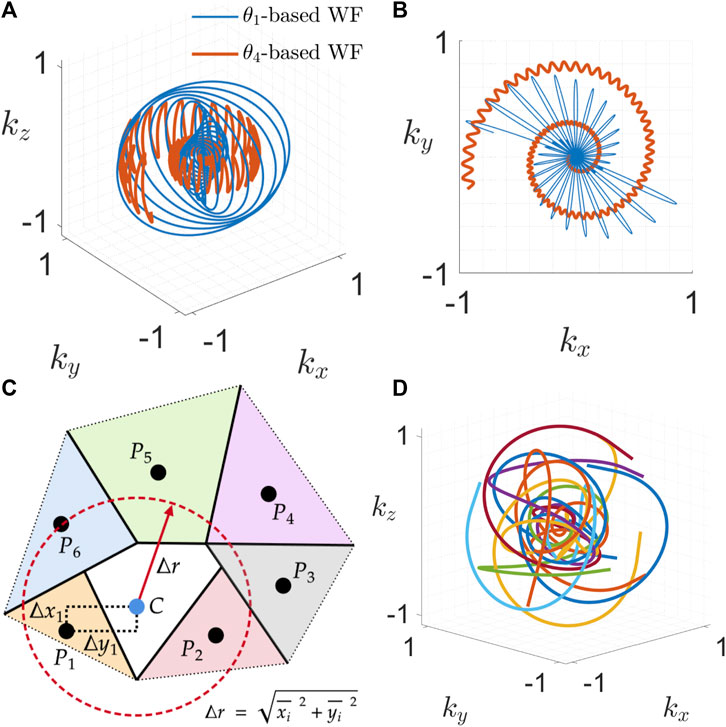
FIGURE 1. Two interleaves, each based on a different Jacobi theta function θ₁ and θ₄. Both interleaves are shown in three-dimensional k-space (A) and as a plane projection in (B). (C) Schematic representation of seven Voronoi cells in a two-dimensional k-space. Six nearest neighbours of the point of interest C are used for the definition of the generalised FOV. (D) Ten interleaves of the presented 3D ζ-based Spiral trajectory. The increased sampling density around the centre of k-space can be clearly appreciated.

In order to calculate a local estimate of the encoded FOV at C, the direct distances $d_{C,P_i}$ between C and each P_i are calculated and the mean value of all six distances defines a radius Δr around C. This radius can then define a generalised FOV for C with FOV_C = 1/Δr_C but in the same manner also for every other point in k-space. In the three dimensional case, Δr defines the radius of a sphere, from which an equal FOV along each direction is derived. For this calculation, a sufficient number of nearest neighbours is required, to ensure that Δr is derived from the expression $\mathrm{\Delta }r=\sqrt{{\overline{\mathrm{\Delta }{x}_i}}^2+{\overline{\mathrm{\Delta }{y}_i}}^2+{\overline{\mathrm{\Delta }{z}_i}}^2}$ with Δx_i ≠ 0, Δy_i ≠ 0 and Δz_i ≠ 0, i.e. the radius can define a spherical (3D) volume. The given definition also allows the assignment of an isotropic FOV for various specific regions in k-space as well as for the entire trajectory by averaging Δr for all considered k-space points.

Methods

Interleaves in k-Space Based on Theta Functions

The previous publication [17] has used Jacobi elliptic functions for the construction of a single k-space interleave as the solution to an optimisation problem given by P. Erdös in 2000 [19]. Here, we have generalised the approach by making use of Jacobi theta functions [20], giving rise to the possibility of constructing a multitude of inherently different k-space waveforms. For example, Figure 1A shows two different k-space waveforms of arbitrary length, for which the k_x − and k_y − components are once based on θ₁ and once based on θ₄ (k_z = θ₂). A projection of both waveforms into the k_x − k_y − plane is shown in Figure 1B. All corresponding gradient waveforms are shown in Figure 2.

FIGURE 2

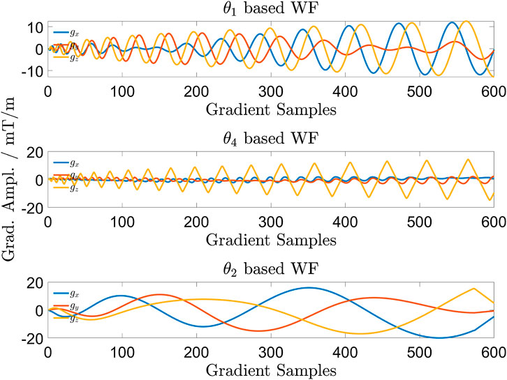
FIGURE 2. All gradient channels of one interleave of the three trajectories shown in Figure 1. Due to different interleave lengths, the first 600 points of each gradient waveform are shown. The θ₂ based gradient waveform refers to 1d).

The waveform presented in the following is meant to prove the imaging concept for a lower limit of read-out durations and is generally based on the concepts and parameters introduced in [17]. The general waveform is generated on the surface of a unit sphere according to the definition: $\zeta :{\mathbb{R}}_0^{+}\to {\mathbb{R}}^3$, s↦ζ(s) with η ∈ (0, 1) and

${\zeta }_x\left(s,\eta \right)={\theta }_1\left(s,{\eta }^2\right)\cdot \cos \left(s\cdot {\eta }^2\right)(1)$

${\zeta }_y\left(s,\eta \right)={\theta }_1\left(s,{\eta }^2\right)\cdot \sin \left(s\cdot {\eta }^2\right)(2)$

${\zeta }_z\left(s,\eta \right)={\theta }_2\left(s,{\eta }^2\right)(3)$

While η is a parameter to adapt the waveform to hardware limitations such as maximum gradient amplitudes and available slew-rates. The combination with sine and cosine terms in the first two components allows for a modifiable change in direction per unit length while the symmetry along the z-direction remains unchanged (Figures 1A,B). The length of the waveform is determined by s and therefore the restriction s ∈ [0, s_max] should be applied, with s_max being sufficiently large according to the desired resolution (extension of k-space).

For this publication, one k-space interleave was constructed with η = 0.5 and by setting the target resolution to 0.85 mm (isotropic). For an extended oversampling of k-space centre α = 1.3 was chosen to facilitate a subsequent CS reconstruction. Each presented trajectory was generated with a maximum gradient strength of 21 mT/m and a slew-rate of 120 T/m/s. Each trajectory was furthermore explicitly optimised by minimising its discrepancy [17], by iterative optimisation of s, η and the angle of rotation around the symmetry axis according to [17] and using an Euclidian arc-length parameterization [21]. An adequate choice of the centre-oversampling parameter α requires information about the energy distribution of the underlying k-space and can therefore not be generally included to the optimisation problem. Nevertheless, defining an interval by experience e.g. α ∈ [1.2, 1.7] allows for another degree of freedom during the optimisation process and is therefore recommended.

The resulting read-out duration for each interleave was 3.52 ms, in order to reach the boundary of the k-space sphere for the defined maximum gradient amplitude and slew-rate limits. Ten interleaves of a final trajectory with 20,000 interleaves are depicted in Figure 1D for illustrative purposes. For this trajectory, we define an undersampling factor of R: = 1 due to an equal scan time as the corresponding Cartesian acquisition at the same resolution and FOV.

Sampling Point Spread Function

Based on the previously mentioned parameters, four sampling point spread functions were calculated according to undersampling factors of R = 1, 8, 12, 16 with respect to the trajectory with the largest number of interleaves, i.e. 20,000. Each trajectory for each undersampling factor was independently generated and optimised with respect to low-coherent sampling properties. All PSF_Ss were obtained by a separate calculation of a Voronoi tessellation [7] in Euclidean space (${\mathbb{R}}^3$, Euclidean distance) for every generated trajectory. Each PSF_S was obtained by gridding unit k-space data onto a Cartesian grid in combination with a 3D Voronoi tessellation [17, 22] to estimate weights for the necessary density compensation of non-uniformly acquired k-space data. Based on all normalised PSF_Ss, the centre-peak FWHM was determined in order to evaluate relative image sharpness with increasing undersampling factors. Furthermore, the peak/side-lobe ratio

$\text{PSR}=\underset{i\ne j}{\max }\left|\frac{{\text{PSF}}_{\text{S}}\left(i,j\right)}{{\text{PSF}}_{\text{S}}\left(i,i\right)}\right|(4)$

Of each PSF_S is an appropriate measure for emerging coherences [3].

In-Vivo Imaging and Reconstruction

In order to evaluate the aliasing behaviour, as well as imaging performance, in-vivo head images were acquired using a 3.0 T wholebody MRI system (Achieva 3.0 T, Philips, Best, Netherlands) with an 8-element SENSE Neuro coil (Philips, Best, Netherlands).

Image reconstruction for all 3D ζ-based Spirals was performed as follows: after data acquisition, raw data were exported and processed with MATLAB (MathWorks, Natick, MA, United States). Images were obtained using gridding [23] with an oversampling factor of 1.25, a Kaisser Bessel kernel for interpolation and again in combination with a 3D Voronoi tessellation. Gradient system delays were estimated [24] and used to correct the trajectory before gridding. Further eddy current effects were compensated using a mono-exponential model [25] with a time constant of τ = 39 μs. No post-processing was applied to any of the presented image. Compressed Sensing reconstructions were accomplished using an in-house written CS/SENSE reconstruction based on nonlinear conjugate gradient methods as suggested in [3, 26]. Undersampling was again realized by calculating separate and optimised trajectories with 12,000, 8,000, 4,000 and 1,250 interleaves, leading to undersampling factors R = 1.66, 2.5, 5 and 16 with respect to the initial trajectory with 20,000 interleaves. These undersampling factors were chosen to correspond to scan durations of 90, 60, 30 and 10s. All relevant scan parameters are listed in Table 1.

TABLE 1

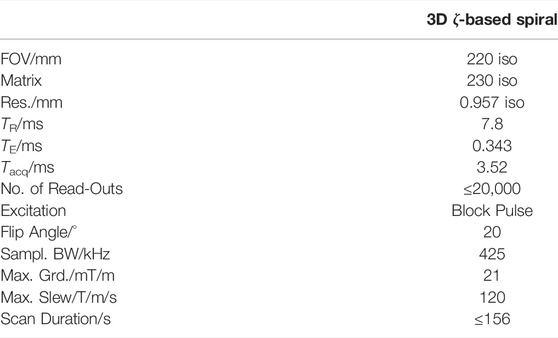
TABLE 1. Scan parameters for all 3D ζ-based Spiral acquisitions.

Undersampling Behaviour and Noise Analysis

To provide an experimental assessment of the aliasing properties, we evaluate the noise characteristics of the acquired in-vivo datasets for the 3D ζ-based Spiral, acquired with 12,000, 8,000, 4,000 and 1,250 interleaves each, according to the previous section. A reference dataset with the vendor’s 3D radial Kooshball trajectory was acquired, employing the same spatial resolution and choosing a FOV encompassing the entire head. Image reconstruction for the Kooshball trajectory followed the description given in the previous section for the 3D ζ-based Spiral trajectory, except for the weighting calculation. Kooshball weights were calculated analytically, based on the symmetry of the sampling scheme (spherical shells). The radial dataset was retrospectively undersampled by a random selection of 1/R spokes.

Three regions of interest (ROI) as highlighted in Figure 3D were selected in the background of the reconstructed images, ideally containing no source of any MR signal. Accordingly, the pixel intensities are exclusively governed by artefacts and noise whose characteristics can be analysed by consideration of the associated power spectrum. The calculation of the power spectrum followed [27], generalised to the 3D case. To facilitate the analysis of their characteristics (line shapes), all power spectra were normalised and are presented in arbitrary units. For each acquisition, the power spectra were averaged over all coil elements and evaluated with respect to the three geometrical axis to capture possible similarities (coherences).

FIGURE 3

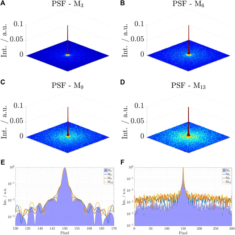
FIGURE 3. Spectral noise analysis for three different ROIs as indicated in d) for four different undersampling factors (ROI 1: green, ROI 2: red, ROI 3: yellow).

Results

Trajectory Properties

According to the definition of the generalised FOV, the presented trajectory with 20,000 interleaves has the following properties: The Nyquist condition Δr_C ≤ 1/FOV = (1/220) mm is fulfilled within a sphere of radius r_N = 0.18 ⋅ k_max. The largest FOV that is stored within a sphere of radius r = 0.01 ⋅ k_max corresponds to 38-times the FOV dimension (220 mm). According to the definition, the Nyquist condition is not fulfilled for points outside a sphere of radius r_N.

Since the number of interleaves for the trajectory with 20,000 interleaves was selected such that the resulting scan duration is approximately equal to a standard Cartesian acquisition (174 s), without considering the actually encoded FOV, it is reasonable to calculate the introduced generalised FOV for this and for all other trajecories, to achieve undersampling factors that truly rely on Nyquist’s condition and not on a relative number of interleaves. Therefore, the trajectory with 20,000 interleaves corresponds to an undersampling factor of $R_1^{\prime }\approx 3.29$. This value was determined by calculating the mean generalised FOV of all sampling points of each trajectory, stating that Nyquist’s theorem is violated 3.29-times according to the definitions. Accordingly, the equally generated trajectory with 2,500 interleaves led to $R_2^{\prime }\approx 6.43$, to $R_3^{\prime }\approx 9.33$ for 1,665 interleaves and to $R_4^{\prime }\approx 12.98$ for 1,250 interleaves. The intention of these numbers is merely to classify the presented trajectories than to enforce comparisons to other sampling schemes due to drastic differences in the distribution of points in k-space. For simplification, all images and results that correspond to undersampling factors $R_1^{\prime },\dots ,R_4^{\prime }$ of the 3D ζ-based Spirals are denoted by M₃, M₆, M₉, M₁₃ according to the mean undersampling factors.

Figure 4 shows all associated sampling point spread functions for these four cases of undersampling in the xy-plane with z = 0.

FIGURE 4

FIGURE 4. Simulated PSF_Ss in the xy-plane with z = 0 of the presented 3D ζ-based Spiral trajectory. The PSF_S in (A) corresponds to 3.29-fold undersampling, the PSF_S in (B) to 6.43-fold undersampling, (C,D) to 9.33-fold and 12.98-fold undersampling respectively. Logarithmic plot of the centre region of all four sampling point spread functions shown in (E) and the same for the entire cross section in (F).

With increasing undersampling, energies in the PSF_Ss emerge that do not seem to follow any ordered or symmetric pattern. Consequently, all PSF_Ss appear to be governed by a low-coherent distribution of energies with an expected aliasing behaviour that is (in its appearance) vastly similar to an introduction of white noise.

Figures 4E,F shows a logarithmic plot of the centre region of the four PSF_Ss, shown in Figures 4A–D and a cross section of the entire PSF_S in 3b). As the undersampling factor increases, an overall increase in energy can be appreciated in which the side-lobe behaviour shows rarely signs of emerging coherences. Furthermore, image sharpness is preserved for all undersampling factors. The FWHM of the PSF_S centre-peak results to $\approx 2.544$  pixel in width (mean) with a maximum deviation of 0.59% between the broadest peak (M₁₃: 2.549 px) and the narrowest peak (M₉: 2.534 px) of all undersampling PSF_Ss. All values were obtained in non-logarithmic representation. This finding of retained sharpness is furthermore supported by the in-vivo images, presented in the following section.

Aliasing Behaviour and Noise Analysis

Figure 5 shows axial and sagittal slices, acquired with the presented 3D ζ-based Spiral trajectories for different numbers of interleaves (20,000, 8,000 and 1,250). All data was directly gridded and no additional image or data processing was applied before and after gridding. Furthermore, no sensitivity maps were used, in order not to alter the emerging imaging artefacts. Figure 5 also shows a Compressed Sensing reconstruction based on the dataset with 1,250 interleaves using a total variation regularisation [7].

FIGURE 5

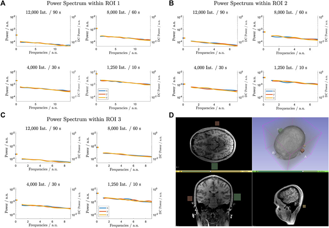
FIGURE 5. Reconstructed axial and sagittal slices from an in-vivo 3D ζ-based Spiral acquisition. The undersampling factor increases from top to bottom. The calculated generalized FOV of each trajectory is indicated as red squares on the sagittal slices. The bottom line shows a Compressed Sensing reconstruction based on the acquisition with 1,250 interleaves.

The generalised FOV for 20,000 interleaves is $\approx 67$ mm (M₃, isotropic), $\approx 41$ mm for 8,000 interleaves and $\approx 17$ mm for 1,250 interleaves (M₁₃). The reconstruction of a larger FOV, in this case of 220 mm (isotropic) for all datasets results in additional low-coherent aliasing artefacts, which can clearly be appreciated. Despite uncorrected coil sensitivity profiles, all images appear non-degraded by coherent aliasing artefacts, especially visible in the background of all images. As expected from the PSF_S analysis, image sharpness is preserved, and based on the optical impression, equal for all investigated undersampling factors.

The noise analysis for the three cubic regions (ROI) is shown in Figure 3. The normalised power spectra indicate slightly overpronounced DC components for all acquisitions. For the 3D ζ-based Spiral trajectories (20,000, 8,000, 4,000 and 1,250 interleaves), all further spatial frequency components are about equally represented, leading to a widely flat power spectrum in accordance to the behaviour of (bandwidth limited) white noise. As expected, an increasing undersampling factor increases the overall power, but the characteristics (line-shapes) remain widely unchanged. Concerning the Kooshball trajectory, with the analysis being shown in the Supplemental Data (Supplementary Figure S1), all directions show a similar behaviour in terms of overpronounced DC components and a following decline of the power spectrum. But, all directions in each evaluated ROI show clear modulations (wave pattern) in the frequency analysis with again increasing powers as the undersampling factor increases. The latter also introduces obvious changes to the frequency modulations, indicating varying (coherent) aliasing artefacts. While the noise-like characteristics of aliasing artefacts remain unchanged for varying undersampling factors in the case of 3D ζ-based Spiral trajectories, undersampling of the radial Kooshball trajectory introduces streak artefacts.

Calculating the peak/side-lobe ratios for the four PSF_ss shown in Figure 4 yields ratios in non-logarithmic representation of 4.7 ⋅ 10^–3 (M₃), 5.1 ⋅ 10^–3 (M₆), 5.2 ⋅ 10^–3 (M₉), 5.8 ⋅ 10^–3 (M₁₃), indicating that emerging coherences remain at the same level with increasing power densities in the PSF_ss towards the outer regions as R increases. Compared to Kooshball sampling with the PSF_ss shown in the Supplemental Data (Supplementary Figure S2), the peak/side-lobe ratio for R = 3 is 5.3 ⋅ 10^–3 while it increases to 11.2 ⋅ 10^–3 for R = 6, to 13.8 ⋅ 10^–3 for R = 9 and to 20.6 ⋅ 10^–3 for R = 13, which is in accordance to the visually enhanced coherences in the emerging aliasing artefacts for increasing undersampling factors.

Discussion and Conclusion

In summary, all presented results show dominant low-coherent aliasing properties, leading to a noise-like aliasing behaviour, which facilitates new imaging strategies or ways in which available scan times can be exploited.

Besides obvious advantages in scan time reduction, by a combination of undersampling with a Compressed Sensing reconstruction, the trajectory is created independent of an application dependent FOV which does therefore not influence the total imaging duration. Using 3D ζ-based Spirals, a trajectory might be constructed just by following given time restrictions and imaging constraints, e.g. such as:

• Size of k-space sphere as defined by the desired image resolution.

• Maximum read-out duration (spiral length) as defined (limited) by off-resonance behaviour and relaxation effects.

• Total acceptable scan duration defines the number of possible interleaves.

Based on the measured dataset, any feasible FOV can then be reconstructed under emerging low-coherent aliasing artefacts if the condition Δr_C ≤ 1/FOV_p is not fulfilled for every point in k-space. Since the reconstructed FOV is defined by the underlying Cartesian grid (gridding/interpolation) and not by the trajectory itself, the same Voronoi density compensation can be used for any reconstructed FOV.

The overall image sharpness (PSF_S FWHM) is highly influenced by the quality of the Voronoi tessellation. It is therefore explicitly important to consider the trade-off between numerical runtime of the volume calculation and the resulting image qualities. All presented images were reconstructed using a not approximated tessellation, based on a thorough Dirichlet tessellation, at the cost of long reconstruction times. In order to achieve a fast optimisation of the trajectory to specific applications, more efficient implementations are desirable. Nevertheless, only one k-space trajectory is required for each specific resolution, since the desired imaging FOV does neither influence the generation of the gradient waveforms nor the entire k-space trajectory itself.

The spectral analysis, as shown in Figure 5, exhibits an overestimation of the DC component for all analysed acquisitions. As the DC component in the power spectrum corresponds to a constant pixel intensity offset, it does not influence the characteristics of the artefacts and might easily be corrected.

The presented approach based on Jacobi theta functions represents a generalised approach to the previously published trajectory design. While it can embody all properties of the Seiffert Spirals, it also derives the possibility of constructing a multitude of new k-space sampling schemes, which are to be discussed in detail in a future publication. All shown results indicate a clear low-coherent aliasing behaviour, based on the underlying generation algorithm.

Data Availability Statement

The raw data supporting the conclusions of this article will be made available by the authors, without undue reservation.

Author Contributions

TS and PM performed the measurements, designed the concept and wrote the first draft of the manuscript. TH and KS contributed to the acuqisition and reconstruction of the shown data. All authors contributed to manuscript revision, read, and approved the submitted version.

Funding

This project has received funding from the European Union’s Horizon 2020 research and innovation programme under grant agreement No 858149. The presented research was also partially funded by Philips Healthcare. The authors thank the Ulm University Centre for Translational Imaging MoMAN for its support.

Conflict of Interest

The authors declare that the research was conducted in the absence of any commercial or financial relationships that could be construed as a potential conflict of interest.

Publisher’s Note

All claims expressed in this article are solely those of the authors and do not necessarily represent those of their affiliated organizations, or those of the publisher, the editors and the reviewers. Any product that may be evaluated in this article, or claim that may be made by its manufacturer, is not guaranteed or endorsed by the publisher.

Supplementary Material

The Supplementary Material for this article can be found online at: https://www.frontiersin.org/articles/10.3389/fphy.2022.867676/full#supplementary-material

References

1. Griswold MA, Jakob PM, Heidemann RM, Nittka M, Jellus V, Wang J, et al. Generalized Autocalibrating Partially Parallel Acquisitions (Grappa). Magn Reson Med (2002) 47:1202–10. doi:10.1002/mrm.10171

PubMed Abstract | CrossRef Full Text | Google Scholar

2. Pruessmann KP, Weiger M, Scheidegger MB, Boesiger P. Sense: Sensitivity Encoding for Fast Mri. Magn Reson Med (1999) 42:952–62. doi:10.1002/(sici)1522-2594(199911)42:5<952::aid-mrm16>3.0.co;2-s

PubMed Abstract | CrossRef Full Text | Google Scholar

3. Lustig M, Donoho D, Pauly JM. Sparse MRI: The Application of Compressed Sensing for Rapid MR Imaging. Magn Reson Med (2007) 58:1182–95. doi:10.1002/mrm.21391

PubMed Abstract | CrossRef Full Text | Google Scholar

4. Foucart S, Rauhut H. A Mathematical Introduction to Compressive Sensing, Vol. 1. Basel: Birkhäuser Basel (2013).

Google Scholar

5. Levine E, Daniel B, Vasanawala S, Hargreaves B, Saranathan M. 3D Cartesian MRI with Compressed Sensing and Variable View Sharing Using Complementary Poisson-Disc Sampling. Magn Reson Med (2017) 77:1774–85. doi:10.1002/mrm.26254

PubMed Abstract | CrossRef Full Text | Google Scholar

6. Hollingsworth KG. Reducing Acquisition Time in Clinical MRI by Data Undersampling and Compressed Sensing Reconstruction. Phys Med Biol (2015) 60:R297–322. doi:10.1088/0031-9155/60/21/R297

PubMed Abstract | CrossRef Full Text | Google Scholar

7. Speidel T, Paul J, Wundrak S, Rasche V. Quasi-random Single-point Imaging Using Low-Discrepancy K-Space Sampling. IEEE Trans Med Imaging (2018) 37:473–9. doi:10.1109/tmi.2017.2760919

PubMed Abstract | CrossRef Full Text | Google Scholar

8. Sherry F, Benning M, De los Reyes JC, Graves MJ, Maierhofer G, Williams G, et al. Learning the Sampling Pattern for Mri. IEEE Trans Med Imaging (2020) 39:4310–21. doi:10.1109/tmi.2020.3017353

PubMed Abstract | CrossRef Full Text | Google Scholar

9. Chauffert N, Ciuciu P, Kahn J, Weiss P Variable Density Sampling with Continuous Trajectories. SIIMS. (2014) 7(4):1962–1992. doi:10.1109/tmi.2019.2892378

PubMed Abstract | CrossRef Full Text | Google Scholar

10. Senel LK, Kilic T, Gungor A, Kopanoglu E, Guven HE, Saritas EU, et al. Statistically Segregated K-Space Sampling for Accelerating Multiple-Acquisition Mri. IEEE Trans Med Imaging (2019) 38:1701–14. doi:10.1109/tmi.2019.2892378

PubMed Abstract | CrossRef Full Text | Google Scholar

11. Prieto C, Doneva M, Usman M, Henningsson M, Greil G, Schaeffter T, et al. Highly Efficient Respiratory Motion Compensated Free-Breathing Coronary Mra Using golden-step Cartesian Acquisition. J Magn Reson Imaging (2015) 41:738–46. doi:10.1002/jmri.24602

PubMed Abstract | CrossRef Full Text | Google Scholar

12. Pipe JG, Zwart NR, Aboussouan EA, Robison RK, Devaraj A, Johnson KO. A New Design and Rationale for 3D Orthogonally Oversampled K -space Trajectories. Magn Reson Med (2011) 66:1303–11. doi:10.1002/mrm.22918

PubMed Abstract | CrossRef Full Text | Google Scholar

13. Lazarus C, Weiss P, Chauffert N, Mauconduit F, El Gueddari L, Destrieux C, et al. SPARKLING: Variable-Density K-Space Filling Curves for Accelerated T2 * -weighted MRI. Magn Reson Med (2019) 81:3643–61. doi:10.1002/mrm.27678

PubMed Abstract | CrossRef Full Text | Google Scholar

14. Gurney PT, Hargreaves BA, Nishimura DG. Design and Analysis of a Practical 3d Cones Trajectory. Magn Reson Med (2006) 55:575–82. doi:10.1002/mrm.20796

PubMed Abstract | CrossRef Full Text | Google Scholar

15. Johnson KM. Hybrid Radial-Cones Trajectory for Accelerated Mri. Magn Reson Med (2017) 77:1068–81. doi:10.1002/mrm.26188

PubMed Abstract | CrossRef Full Text | Google Scholar

16. Irarrazabal P, Nishimura DG. Fast Three Dimensional Magnetic Resonance Imaging. Magn Reson Med (1995) 33:656–62. doi:10.1002/mrm.1910330510

PubMed Abstract | CrossRef Full Text | Google Scholar

17. Speidel T, Metze P, Rasche V. Efficient 3D Low-Discrepancy K-Space Sampling Using Highly Adaptable Seiffert Spirals. IEEE Trans Med Imaging (2019) 38:1833–40. doi:10.1109/tmi.2018.2888695

PubMed Abstract | CrossRef Full Text | Google Scholar

18. Stobbe RW, Beaulieu C. Three-dimensional Yarnball K-Space Acquisition for Accelerated Mri. Magn Reson Med (2021) 85:1840–54. doi:10.1002/mrm.28536

PubMed Abstract | CrossRef Full Text | Google Scholar

19. Erdös P. Spiraling the Earth with C. G. J. Jacobi. Am J Phys (2000) 68:888–95. doi:10.1119/1.1285882

CrossRef Full Text | Google Scholar

20. Abramowitz M, Stegun IA. Handbook of Mathematical Functions with Formulas, Graphs, and Mathematical Tables. Washington: Dover Publications (1965).

Google Scholar

21. Lustig M, Kim S-J, Pauly JM. A Fast Method for Designing Time-Optimal Gradient Waveforms for Arbitrary K-Space Trajectories. IEEE Trans Med Imaging (2008) 27:866–73. doi:10.1109/tmi.2008.922699

PubMed Abstract | CrossRef Full Text | Google Scholar

22. Rasche V, Proksa R, Sinkus R, Bornert P, Eggers H. Resampling of Data between Arbitrary Grids Using Convolution Interpolation. IEEE Trans Med Imaging (1999) 18:385–92. doi:10.1109/42.774166

PubMed Abstract | CrossRef Full Text | Google Scholar

23. Beatty PJ, Nishimura DG, Pauly JM. Rapid Gridding Reconstruction with a Minimal Oversampling Ratio. IEEE Trans Med Imaging (2005) 24:799–808. doi:10.1109/tmi.2005.848376

PubMed Abstract | CrossRef Full Text | Google Scholar

24. Robison RK, Devaraj A, Pipe JG. Fast, Simple Gradient Delay Estimation for Spiral Mri. Magn Reson Med (2010) 63:1683–90. doi:10.1002/mrm.22327

PubMed Abstract | CrossRef Full Text | Google Scholar

25. Atkinson IC, Lu A, Thulborn KR. Characterization and Correction of System Delays and Eddy Currents for Mr Imaging with Ultrashort echo-time and Time-Varying Gradients. Magn Reson Med (2009) 62:532–7. doi:10.1002/mrm.22016

PubMed Abstract | CrossRef Full Text | Google Scholar

26. Fessler JA. Optimization Methods for Mr Image Reconstruction (Long Version) (2019). arXiv preprint arXiv:1903.03510. doi:10.48550/ARXIV.1903.03510

CrossRef Full Text | Google Scholar

27. Van der Schaaf A, van Hateren JH. Modelling the Power Spectra of Natural Images: Statistics and Information. Vis Res (1996) 36:2759–70. doi:10.1016/0042-6989(96)00002-8

PubMed Abstract | CrossRef Full Text | Google Scholar