The Solution Comparison of Time-Fractional Non-Linear Dynamical Systems by Using Different Techniques

This comparative study of fractional nonlinear fractional Burger’s equations and their systems has been done using two efficient analytical techniques. The generalized schemes of the proposed techniques for the suggested problems are obtained in a very sophisticated manner. The numerical examples of Burger’s equations and their systems have been solved using Laplace residual power series method and Elzaki transform decomposition method. The obtained results are compared through graphs and tables. The error tables have been constructed to show the associated accuracy of each method. The procedures of both techniques are simple and attractive and, therefore, can be extended to solve other important fractional order problems.

1 Introduction

The branch of mathematics that deals with the study of derivatives and integrals of non-integer orders is known as fractional calculus (FC). It originated on 30 September 1695 due to an important question asked by L’Hospital in a letter to Leibniz. The answer of Leibniz [1] gives motivation to a series of interesting results during the last 325 years [2–4]. In the last decades, FC has been used as a powerful tool by many researchers in various fields of science and engineering, for example, the fractional control theory [2, 5], anomalous diffusion, fractional neutron point kinetic model, fractional filters, soft matter mechanics, non-Fourier heat conduction, notably control theory, Levy statistics, nonlocal phenomena, fractional signal and image processing, porous media, fractional Brownian motion, relaxation, groundwater problems, rheology, acoustic dissipation, creep, fractional phase-locked loops, and fluid dynamics [6–12].

In recent years, Fractional Partial Differential Equations (FPDEs) have gained considerable interest because of their applications in various fields such as finance, biological processes and systems, fluid flow [13, 14], chaotic dynamics, electrochemistry, diffusion processes, material science, electromagnetic, turbulent flow [15–20], elastoplastic indentation problems [21], dynamics of van der Pol equation [22], and statistical mechanics model [23].

Finding the solution to FPDEs is a hard task. However, many mathematicians devoted their sincere work and developed numerical and analytical techniques to solve FPDEs. Some of these techniques include homotopy analysis method (HAM) [24], operational matrix [25], Adomian decomposition method (ADM) [26], homotopy perturbation method (HPM) [27], meshless method [28], variational iteration method (VIM) [29], tau method [30], Bernstein polynomials [31], the Haar wavelet method [32], the Laplace transform method [33], the Legendre base method [34], Laplace variational iteration method [35], G’/G-expansion method [36], Jacobi spectral collocation method [37], Yang–Laplace transform [38], new spectral algorithm [39], fractional complex transform method [40], cylindrical-coordinate method [41], and spectral Legendre–Gauss–Lobatto collocation method [42]. Yusufoglu et al. presented the solutions of the equal-with-wave equation and gBBM equation using various techniques [43, 44]. Bakir et al. used the traveling waves solutions idea for KdV-mKdV and modified Burger–KdV equation in [45]. Kaplan et al. [46, 47] investigated the solutions of conformable equations and Benjamin–Ono equation with the help of generalized Kudryashov techniques and the exp ( − ϕ(ξ)) method, respectively.

Burger’s equation was initially introduced by Harry Bateman in 1915 [48]. They have many applications in various fields, especially in equations with non-linear forms. This equation describes many phenomena such as acoustic waves, heat conduction, dispersive water, shock waves [49], continuous stochastic processes [50], and modeling of dynamics [51–53]. The one-dimensional Burger’s equations have many applications in plasma physics, gas dynamics, and so on [54]. Various techniques were developed by mathematicians to find the numerical and analytical solutions to Burger’s equations. Some of these methods are a direct variational iteration method by [55, 56] solving the equations numerically by the finite difference method. The group explicit method was used by [57]. Singhal and Mittal applied the Galerkin method [58] to solve these equations numerically. A weighted residue method was applied by [59]. The fractional Riccati expansion method was applied by [60], and the variational iteration method was applied by Inc [61] to solve space-time fractional Burger’s equation. Esen et al. [62] used HAM to solve the time-fractional Burger equation. The Cubic B-spline finite elements method was applied by Esen et al. to solve these equations [63].

In the present article, we will use the Elzaki transform decomposition method (ETDM) and Laplace residual power series method (LRPSM) to solve Burger’s equation with one and two dimensions. The ETDM was introduced by [64] in 2010, which is the combination of ADM [65] and Elzaki transforms (ET). The ET is a modified transformation of Sumudu (ST) and Laplace transformation (LT). Many differential equations with variable coefficients cannot be solved by LT and ST so that equations can be easily managed by ET [66]. Many mathematicians applied ET to solve various kinds of Fisher [67], Navier–Stokes [68], heat-like [69] equations.

LRPSM combines the LT and Residual power series method (RPSM), giving the exact and approximate solution as a power series solution that is rapidly convergent. This technique was developed for the first time in [70] and applied in [71]. LRPSM is a technique that requires fewer computations and time with more accuracy.

This work applies ETDM and LRPSM to Burger’s equations of one and two dimensions. Some numerical examples are solved by both methods. The results obtained by these two methods will be compared by making plots and tables for each problem, and then a comparison is made by making combined plots and tables for these two methods. The proposed techniques are more accurate and simple and require fewer calculations than other exciting methods. These techniques need no discretization or extra parameters to obtain the solutions to the problems. The current techniques have the unique capability to utilize the Laplace transformation to reduce the given model into its simple form. The simple series form solutions of the suggested techniques are achieved with easily computable and convergent components. The present techniques provide higher accuracy despite using very few terms of the series solution.

2 Preliminaries

In this section, a few definitions related to our work are considered.

2.1 Definition

The Caputo time-fractional derivative is defined as [2]

$\begin{array}{ll}\hfill D_t^{\beta }\mu \left(\xi ,t\right)& =\frac{1}{\mathrm{\Gamma }\left(n-\beta \right)}{\int }_0^t{\left(t-\tau \right)}^{n-\beta -1}\frac{{\partial }^n\mu \left(\xi ,\tau \right)}{\partial {\tau }^n}d\tau ,n-1<\beta <n,\hfill \\ \hfill & =\frac{{\partial }^n\mu \left(\xi ,\tau \right)}{\partial t^n},\beta =n,n\in N.\hfill \end{array}$

2.2 Definition

A power series is represented as [3]

$\sum _{n=0}^{\infty }{C}_n{\left(t-t_0\right)}^{n\beta }=C_0+C_1{\left(t-t_0\right)}^{\beta }+C_2{\left(t-t_0\right)}^{2\beta }+\dots ,$

where 0 ≤ n − 1 < β ≤ 1, t ∈ N, and t ≥ t₀ is known as fractional power series about t₀.

2.3 Definition

Consider the expansion as follows [3], known as power series of multiple fraction about t = t₀:

$\sum _{n=0}^{\infty }{g}_m\left(\xi \right){\left(t-t_0\right)}^{n\beta },n-1<\beta <n.$

2.4 Lemma

If μ(ξ, t) is represented as [3] multiple fractions at t = t₀, then

$\begin{array}{l}\hfill \mu \left(\xi ,t\right)=\sum _{n=0}^{\infty }{g}_n\left(\xi \right){\left(t-t_0\right)}^{n\beta },n-1<\beta <n,\\ \hfill \left(\xi ,y\right)\in I_1\times I_2{t}_0\le t<t_0+R.\end{array}$

If $D_t^{n\beta }\mu (\xi ,t)$, n = 0, 1, …. is continuous on I₁ × I₂ × (t₀, t₀ + R), then

$g_m\left(\xi \right)=\frac{D^{m\beta }\mu \left(\xi ,t_0\right)}{\mathrm{\Gamma }\left(1+m\beta \right)}.$

2.5 Corollary

If μ(ξ, y, t) has representation as [3] multiple fractions at t = t₀, then

$\begin{array}{l}\hfill \mu \left(\xi ,y,t\right)=\sum _{n=0}^{\infty }{g}_n\left(\xi ,y\right){\left(t-t_0\right)}^{n\beta },\\ \hfill \left(\xi ,y\right)\in I_1\times I_2{t}_0\le t<t_0+R.\end{array}$

If $D_t^{n\beta }\mu (\xi ,y,t)$, m = 0, 1, 2 … is continuous on I₁ × I₂ × (t₀, t₀ + R), then

$g_m\left(\xi ,y\right)=\frac{D^{m\beta }\mu \left(\xi ,y,t_0\right)}{\mathrm{\Gamma }\left(1+n\beta \right)}.$

2.6 Definition

The Laplace transform of continuous function f(t) in [0, 1) is defined as [1]

$F\left(s\right)=L\left[f\left(t\right)\right]={\int }_0^{\infty }{e}^{-st}f\left(t\right)dt.(1)$

2.7 Definition

The Laplace transform of f(t) = t^α is defined as [1]

$L\left[t^{\alpha }\right]={\int }_0^{\infty }{e}^{-st}{t}^{\alpha }dt=\frac{\mathrm{\Gamma }\left(\alpha +1\right)}{s^{\alpha +1}}R\left(s\right)>0,R\left(\alpha \right)>0n-1<\alpha <n.(2)$

2.8 Definition

The Mittag-leffler function E_α with α > 0 is defined as [1]

$E_{\alpha }\left(z\right)=\sum _{n=0}^{\infty }\frac{z^{\alpha }}{\mathrm{\Gamma }\left(n\alpha +1\right)}\alpha >0,z\in \mathbf{C}.(3)$

2.9 Definition

If ϕ ∈ H [0, T], T > 0, r ∈ (0, 1), then Caputo–Fabrizio of fractional derivative is expressed as [1]

${}_0{}^{CF}D_{\tau }^r\left[\varphi \left(\tau \right)\right]=\frac{M\left(r\right)}{1-r}{\int }_0^{\tau }{\varphi }^{\prime }\left(\zeta \right)K\left(\tau ,\zeta \right)d\zeta ,$

where M(r) is the normalization function with M(1) = M(0) = 1. If ϕ ∈ H [0, T],

${}_0{}^{CF}D_{\tau }^r\left[\varphi \left(\tau \right)\right]=\frac{M\left(r\right)}{1-r}{\int }_0^{\tau }\left(\varphi \left(\tau \right)-\varphi \left(\zeta \right)\right)\left(\zeta \right)K\left(\tau ,\zeta \right)d\zeta .$

2.10 Definition

The Caputo–Fabrizio of fractional integral due to r ∈ (0, 1) is defined as [1]

${}_0{}^{CF}I_{\tau }^r\left[\varphi \left(\tau \right)\right]=\frac{1-r}{M\left(r\right)}\varphi \left(\tau \right)+\frac{r}{M\left(r\right)}{\int }_0^{\tau }\varphi \left(\zeta \right)d\zeta ,\tau \ge 0.$

2.11 Definition

The Laplace transformation of relation with Caputo–Fabrizio as [29]

$\begin{array}{ll}\hfill \mathit{\pounds }\left[{}_0{}^{CF}D_{\tau }^{r+M}\left[\varphi \left(\tau \right)\right]\right]=& \frac{1}{1-r}\left[{\varphi }^{\left(m+r\right)\left(\tau \right)}\right]\mathit{\pounds }\left\{e^{\frac{-r\tau }{1-r}}\right\}\hfill \\ \hfill =& \frac{1}{s+r\left(1-r\right)}\left\{s^{m+1}\mathit{\pounds }\left(\varphi \left(\tau \right)\right)+\sum _{k=1}^m{s}^{m-k}{g}^k\left(0\right)\right\}.\hfill \end{array}$

If m = 0, 1,

$\begin{array}{ll}\hfill & \mathit{\pounds }\left[{}_0{}^{CF}D_{\tau }^r\left[\varphi \left(\tau \right)\right]\right]=\frac{s\mathit{\pounds }\left\{\varphi \left(\zeta \right)\right\}}{s+r\left(1-s\right)},\hfill \\ \hfill & \mathit{\pounds }\left[{}_0{}^{CF}D_{\tau }^{r+1}\left[\varphi \left(\tau \right)\right]\right]=\frac{s\mathit{\pounds }\left\{\varphi \left(\zeta \right)\right\}+s\varphi \left(0\right)-{\varphi }^{\prime }\left(0\right)}{s+r\left(1-s\right)}.\hfill \end{array}$

2.12 Definition

The Laplace transformation of the Caputo operators is provided by [29]

$\mathit{\pounds }\left[{}_0{}^{CF}D_{\tau }^r\left[\varphi \left(\tau \right)\right]\right]=s\mathit{\pounds }\left\{\varphi \left(\zeta \right)\right\}-\sum _{k=0}^{\rho -1}{s}^{\rho -k-1}{\varphi }^k\left(0\right).$

2.13 Elzaki Transform

ET is the generalized form of the Sumudu transformation, which can be define as [72]

$\epsilon \left[f\left(\vartheta \right)\right]=F\left(q\right)=q{\int }_0^{\infty }f\left(\vartheta \right)e^{\frac{-\vartheta }{q}}d\vartheta ,\vartheta >0.$

The following are the results of ET for certain partial differential equations:

$\begin{array}{ll}\hfill & i.\epsilon \left[\frac{\partial f\left(\zeta ,\vartheta \right)}{\partial \vartheta }\right]=\frac{1}{q}F\left(\zeta ,q\right)-qf\left(\zeta ,0\right).\hfill \\ \hfill ii.\epsilon \left[\frac{{\partial }^{2}f\left(\zeta ,\vartheta \right)}{\partial {\vartheta }^2}\right]=\frac{1}{q^2}F\left(\zeta ,q\right)-f\left(\zeta ,0\right)-q\frac{\partial f\left(\zeta ,0\right)}{\partial \vartheta }\\ \hfill & iii.\epsilon \left[\frac{\partial f\left(\zeta ,\vartheta \right)}{\partial \zeta }\right]=\frac{d}{d\zeta }F\left(\zeta ,q\right).\hfill \\ \hfill & iv.\epsilon \left[\frac{{\partial }^{2}f\left(\zeta ,\vartheta \right)}{\partial {\zeta }^2}\right]=\frac{d^2}{d{\zeta }^2}F\left(\zeta ,q\right).\hfill \end{array}$

3 Methodology of LRPSM and ETDM

3.1 Implementation of LRPSM

To understand the basic concept of this algorithm [70], we consider a particular non-linear FPDEs:

$D_{\tau }^{\beta }\mu \left(\xi ,\tau \right)=N\left(\mu \right)+L\left(\mu \right)+q\left(\xi ,\tau \right),\xi ,\tau \ge 0,m-1<\beta <m,(4)$

where D^βμ(ξ, τ) in Eq. 4 is Caputo–Fabrizio derivatives, while $\mathcal{L}$ and $\mathcal{N}$ are the linear and non-linear operators, respectively, and g (ζ, τ) is the source term.

The initial condition is given as follows:

$\mu \left(\xi ,0\right)=f\left(\xi \right).$

Using the idea of RPSM, Eq. 4 is written as the fractional power series at the initial point τ = 0:

$\mu \left(\xi ,\tau \right)=\sum _{n=0}^{\infty }\frac{f_n\left(\xi \right){\tau }^{n\beta }}{\mathrm{\Gamma }\left(1+n\beta \right)},$

where 0 < β ≤ 1, − ∞ < ξ < ∞, and 0 ≤ τ < R.Let μ_k (ξ, τ) be the kth truncated series of μ(ξ, τ):

${\mu }_k\left(\xi ,\tau \right)=\sum _{n=0}^{\infty }\frac{f_n\left(\xi \right){\tau }^{n\beta }}{\mathrm{\Gamma }\left(1+n\beta \right)}.(5)$

The 0th RPS approximation is

${\mu }_0\left(\xi ,\tau \right)=\mu \left(\xi ,0\right)=f\left(\xi \right).$

Eq. 5 is written as

${\mu }_k\left(\xi ,\tau \right)=f\left(\xi \right)+\sum _{n=0}^{\infty }\frac{f_n\left(\xi \right){\tau }^{n\beta }}{\mathrm{\Gamma }\left(1+n\beta \right)},k=\mathrm{1,2},\cdots .(6)$

The residual function for Eq. 4 is defined as

$Re{s}_{\mu }\left(\xi ,\tau \right)=D_{\tau }^{\beta }\mu \left(\xi ,\tau \right)-N\left(\mu \right)-L\left(\mu \right)+q\left(\xi ,\tau \right).$

Therefore, the kth residual function Res_μ,k is

$Re{s}_{\mu ,k}\left(\xi ,\tau \right)=D_{\tau }^{\beta }{\mu }_k\left(\xi ,\tau \right)-L\left({\mu }_k\right)-R\left({\mu }_k\right).(7)$

If Resμ(ξ, τ) = 0 and lim_k→∞Res_k (ξ, τ) = Res(ξ, t), then $D_{\tau }^{n\beta }=0$ because using the Caputo sense, the fractional derivative of a constant is zero and the fractional derivatives $D_t^{n\beta }$ of Res(ξ, t) and Res_k (ξ, τ) are same at τ = 0 for each k = 0, 1, ⋅, k; that is $D_{\tau }^{n\beta }Res(\xi ,0)=D_t^{n\beta }Re{s}_k(\xi ,0),n=\mathrm{0,1},\dots ,k$. To find out f₁(ξ), f₂(ξ), f₃(ξ)…, let k = 0, 1, ⋯ in Eq. 6 and substitute it into Eq. 7, applying fractional derivative $D_{\tau }^{K-1\beta }$ in both sides, k = 1, 2, ⋯ , and finally we solve

$D_{\tau }^{K-1\beta }Re{s}_{\mu ,k}\left(\xi ,0\right)=0,k=\mathrm{0,1},\cdots .$

3.2 Implementation of ETDM

To understand the basic concept of this algorithm [30] , we consider particular non-linear FPDEs:

$D^{\beta }\mu \left(\xi ,\tau \right)+L\mu \left(\xi ,\tau \right)+N\mu \left(\xi ,\tau \right)=q\left(\xi ,\tau \right),\xi ,\tau \ge 0,m-1<\beta <m,(8)$

where D^βμ(ξ, τ) in Eq. 8 is Caputo–Fabrizio derivatives, while $\mathcal{L}$ and $\mathcal{N}$ are the linear and non-linear operators, respectively, and g (ζ, τ) is the source term.The initial condition is as follows:

$\mu \left(\xi ,0\right)=f\left(\xi \right).$

Taking ET to Eq. 8, we have

$\mathcal{E}\left[D^{\beta }\mu \left(\xi ,\tau \right)\right]+\mathcal{E}\left[Lu\left(\xi ,\tau \right)+N\mu \left(\xi ,\tau \right)\right]=\mathcal{E}\left[q\left(\xi ,\tau \right)\right].$

With the help of fractional differential property of ET, we have

$\frac{\mathcal{E}\left[\mu \left(\xi ,\tau \right)\right]}{s^{\beta }}-\sum _{j=0}^{\aleph -1}{s}^{2+j-\beta }\frac{{\partial }^k\mu \left(\xi ,\tau \right)}{{\partial }^k\tau }{|}_{\tau =0}=\mathcal{E}\left[q\left(\xi ,\tau \right)\right]-\mathcal{E}\left[L\mu \left(\xi ,\tau \right)+N\mu \left(\xi ,\tau \right)\right],$

$\mathcal{E}\mu \left(\xi ,\tau \right)=s^2\mu \left(\xi ,0\right)+s^{\beta }\left[\mathcal{E}\left[q\left(\xi ,\tau \right)\right]\right]-s^{\beta }\left[\mathcal{E}\left[L\mu \left(\xi ,\tau \right)+N\mu \left(\xi ,\tau \right)\right]\right],$

and

$\mathcal{E}\left[\mu \left(\xi ,\tau \right)\right]=s^{2}k\left(\xi \right)+s^{\beta }\mathcal{E}\left[q\left(\xi ,\tau \right)\right]-s^{\beta }\mathcal{E}\left[L\mu \left(\xi ,\tau \right)+N\mu \left(\xi ,\tau \right)\right].(9)$

Using ETDM procedure, the solution is expressed as

$\mu \left(\xi ,\tau \right)=\sum _{j=0}^{\infty }{\mu }_j\left(\xi ,\tau \right).(10)$

The nonlinear term can be decompose as

$N\mu \left(\xi ,\tau \right)=\sum _{j=0}^{\infty }{A}_j,(11)$

$A_j=\frac{1}{j!}{\left[\frac{d^j}{d{\lambda }^j}\left[N\sum _{j=0}^{\infty }\left({\lambda }^j{\mu }_j\right)\right]\right]}_{\lambda =0},j=\mathrm{0,1},\cdots$

By substituting Eqs 10–11 in Eq. 9, we get

$\mathcal{E}\left[\sum _{j=0}^{\infty }\mu \left(\xi ,\tau \right)\right]=s^{2}k\left(\xi \right)+s^{\beta }\left[\mathcal{E}\left[q\left(\xi ,\tau \right)\right]\right]-s^{\beta }\left[\mathcal{E}\sum _{j=0}^{\infty }{\mu }_j\left(\xi ,\tau \right)+\sum _{j=0}^{\infty }{A}_j\right],$

$\mathcal{E}\left[{\mu }_0\left(\xi ,\tau \right)\right]=s^2\mu \left(\xi ,0\right)+s^{\beta }\mathcal{E}\left[q\left(\xi ,\tau \right)\right],$

$\mathcal{E}\left[{\mu }_1\left(\xi ,\tau \right)\right]=-s^{\beta }\left[\mathcal{E}\left[{\mu }_0\left(\xi ,\tau \right)+A_0\right]\right].$

Generally, we can write

$\mathcal{E}\left[{\mu }_{j+1}\left(\xi ,\tau \right)\right]=-s^{\beta }\left[\mathcal{E}\left[{\mu }_j\left(\xi ,\tau \right)+A_j\right]\right],j\ge 1.(12)$

Taking the inverse ET of Eq. 12, we have

${\mu }_0\left(\xi ,\tau \right)=f\left(\xi ,\tau \right)+{\mathcal{E}}^{-1}\left[s^{\beta }\mathcal{E}\left[q\left(\xi ,\tau \right)\right]\right],$

${\mu }_{j+1}\left(\xi ,\tau \right)=-{\mathcal{E}}^{-1}\left[s^{\beta }\mathcal{E}\left[{\mu }_j\left(\xi ,\tau \right)+A_j\right]\right].$

4 Numerical Results

4.1 Example

Consider the following one-dimensional time-fractional-order Burger’s equation:

$D_{\tau }^{\delta }\mu ={\mu }_{\zeta \zeta }-\mu {\mu }_{\zeta },0<\delta \le 1.(13)$

Subject to the initial condition,

$\mu \left(\zeta ,0\right)=2\zeta =f_0\left(\zeta \right).(14)$

The exact solution of Eq. 13 is

$\mu \left(\zeta ,\tau \right)=\frac{2\zeta }{1+2\tau }.(15)$

4.1.1 Solution by LRPSM

Applying LT to Eq. 13 and using the initial condition Eq. 14, we get

$\mu \left(\zeta ,s\right)=\frac{2\zeta }{s}-\frac{1}{s^{\delta }}{\mathcal{L}}_{\tau }\left[\left[{\mathcal{L}}_{\tau }^{-1}\mu \left(\zeta ,s\right)\right]\left[{\mathcal{L}}_{\tau }^{-1}{\mu }_{\zeta }\left(\zeta ,s\right)\right]\right]+\frac{{\mu }_{\zeta \zeta }\left(\zeta ,s\right)}{s^{\delta }}.(16)$

The kth truncated term series of Eq. 16 is

${\mu }_k\left(\zeta ,s\right)=\frac{2\zeta }{s}+\sum _{n=1}^k\frac{f_n\left(\zeta \right)}{s^{n\delta +1}}(17)$

and the kth Laplace residual function is

${\mathcal{L}}_{\tau }Re{s}_k\left(\zeta ,s\right)=\mu \left(\zeta ,s\right)-\frac{2\zeta }{s}+\frac{1}{s^{\delta }}{\mathcal{L}}_{\tau }\left[\left({\mathcal{L}}_{\tau }^{-1}\mu \left(\zeta ,s\right)\right)\left({\mathcal{L}}_{\tau }^{-1}{\mu }_{\zeta }\left(\zeta ,s\right)\right)\right]-\frac{{\mu }_{\zeta \zeta }\left(\zeta ,s\right)}{s^{\delta }}.(18)$

Now, to determine f_k(ζ), k = 1, 2, 3, ⋯ , we substitute the kth-truncated series Eq. 17 into the kth-Laplace residual function Eq. 18, multiply the resulting equation by s^kδ+1, and then solve recursively the relation lim_s→∞[s^kδ+1Res_k (ζ, s)] = 0, k = 1, 2, 3, ⋯ , for f_k(ζ). The following are the first few elements of the sequences f_k(ζ):

$\begin{array}{cc}\hfill f_1\left(\zeta \right)& =-4\zeta ,\hfill \\ \hfill f_2\left(\zeta \right)& =16\zeta ,\hfill \\ \hfill f_3\left(\zeta \right)& =16\zeta \frac{\mathrm{\Gamma }\left(2\delta +1\right)}{\mathrm{\Gamma }{\left(\delta +1\right)}^2}-64\zeta ,\hfill \\ \hfill f_4\left(\zeta \right)& =\left[64\zeta \frac{\mathrm{\Gamma }\left(2\delta +1\right)}{\mathrm{\Gamma }{\left(\delta +1\right)}^2}+128\zeta \frac{\mathrm{\Gamma }\left(3\delta +1\right)}{\mathrm{\Gamma }\left(\delta +1\right)\mathrm{\Gamma }\left(2\delta +1\right)}\right],\hfill \\ \hfill & ⋮.\hfill \end{array}(19)$

Putting the values of f_n(ζ) (n ≥ 1) in Eq. 17, we have

$\begin{array}{ll}\hfill \mu \left(\zeta ,s\right)=& \frac{2\zeta }{s}-\frac{4\zeta }{s^{\delta +1}}+\frac{16\zeta }{s^{2\delta +1}}+\left(16\zeta \frac{\mathrm{\Gamma }\left(2\delta +1\right)}{\mathrm{\Gamma }{\left(\delta +1\right)}^2}-64\zeta \right)\frac{1}{s^{3\delta +1}}\hfill \\ \hfill & +\left(64\zeta \frac{\mathrm{\Gamma }\left(2\delta +1\right)}{\mathrm{\Gamma }{\left(\delta +1\right)}^2}+128\zeta \frac{\mathrm{\Gamma }\left(3\delta +1\right)}{\mathrm{\Gamma }\left(\delta +1\right)\mathrm{\Gamma }\left(2\delta +1\right)}\right)\frac{1}{s^{4\delta +1}}+\cdots ,\hfill \end{array}$

$\begin{array}{ll}\hfill \mu \left(\zeta ,s\right)=& 2\zeta \left[\frac{1}{s}-\frac{2}{s^{\delta +1}}+\frac{8}{s^{2\delta +1}}+\left(8\frac{\mathrm{\Gamma }\left(2\delta +1\right)}{\mathrm{\Gamma }{\left(\delta +1\right)}^2}-32\right)\frac{1}{s^{3\delta +1}}\right.\hfill \\ \hfill & +\left.\left(32\zeta \frac{\mathrm{\Gamma }\left(2\delta +1\right)}{\mathrm{\Gamma }{\left(\delta +1\right)}^2}+64\zeta \frac{\mathrm{\Gamma }\left(3\delta +1\right)}{\mathrm{\Gamma }\left(\delta +1\right)\mathrm{\Gamma }\left(2\delta +1\right)}\right)\frac{1}{s^{4\delta +1}}+\cdots \right].\hfill \end{array}$

Applying the inverse Laplace transform, we get

$\begin{array}{ll}\hfill \mu \left(\zeta ,\tau \right)=& 2\zeta \left[1-\frac{2{\tau }^{\delta }}{\mathrm{\Gamma }\left(\delta +1\right)}+\frac{8{\tau }^{\delta }}{\mathrm{\Gamma }\left(2\delta +1\right)}+\left(8\frac{\mathrm{\Gamma }\left(2\delta +1\right)}{\mathrm{\Gamma }{\left(\delta +1\right)}^2}-32\right)\frac{{\tau }^{3\delta }}{\mathrm{\Gamma }\left(3\delta +1\right)}\right.\hfill \\ \hfill & +\left.\left(32\zeta \frac{\mathrm{\Gamma }\left(2\delta +1\right)}{\mathrm{\Gamma }{\left(\delta +1\right)}^2}+64\zeta \frac{\mathrm{\Gamma }\left(3\delta +1\right)}{\mathrm{\Gamma }\left(\delta +1\right)\mathrm{\Gamma }\left(2\delta +1\right)}\right)\frac{{\tau }^{4\delta }}{\mathrm{\Gamma }\left(4\delta +1\right)}+\cdots \right].\hfill \end{array}(20)$

Now, if we substitute δ = 1 in Eq. 20, we have

$\mu \left(\zeta ,\tau \right)=2\zeta \left[1-2\tau +8{\tau }^2-16{\tau }^3+\cdots \right].(21)$

The results given in Eq. 21 agree with the Maclaurin series of

$\mu \left(\zeta ,\tau \right)=\frac{2\zeta }{1+2\tau }.(22)$

4.1.2 Solution by ETDM

Applying ET to Eq. 13 and using the initial condition Eq. 14, we get

$\mathcal{E}\left[\frac{{\partial }^{\delta }\mu }{\partial {\tau }^{\delta }}\right]=\mathcal{E}\left[{\mu }_{\zeta \zeta }-\mu {\mu }_{\zeta }\right].(23)$

With the help of fractional differential property of ET, we have

$\mathcal{E}\left[\mu \left(\zeta ,\tau \right)\right]=s^2\mu \left(\zeta ,0\right)+s^{\delta }\left\{\mathcal{E}\left(\frac{{\partial }^2\mu }{\partial {\zeta }^2}-\frac{\partial \left(\mu \nu \right)}{\partial \zeta }\right)\right\}.(24)$

Applying inverse ET to Eq. 24, we obtain

$\mu \left(\zeta ,\tau \right)=\mu \left(\zeta ,0\right)+{\mathcal{E}}^{-}\left[s^{\delta }\left\{\mathcal{E}\left(\frac{{\partial }^2\mu }{\partial {\zeta }^2}-\frac{\partial \left(\mu \nu \right)}{\partial \zeta }\right)\right\}\right].(25)$

Using the ADM procedure, we get

$\sum _{j=0}^{\infty }{\mu }_j\left(\zeta ,\tau \right)=2\left(\zeta \right)-{\mathcal{E}}^{-1}\left[s^{\delta }\mathcal{E}\left\{\sum _{j=0}^{\infty }{\left({\mu }_{\zeta \zeta }\right)}_j-\sum _{j=0}^{\infty }{A}_j{\left(\mu \nu \right)}_{\zeta }\right\}\right].(26)$

The nonlinear term is represented by the Adomian polynomial A_j (μν)_ζ, where

$\begin{array}{cc}\hfill & A_0{\left(\mu \nu \right)}_{\zeta }=\frac{\partial {\mu }_0}{\partial \zeta }\frac{\partial {\nu }_0}{\partial \zeta },\hfill \\ \hfill & A_1{\left(\mu \nu \right)}_{\zeta }=\frac{\partial {\mu }_0}{\partial \zeta }\frac{\partial {\nu }_1}{\partial \zeta }+\frac{\partial {\mu }_1}{\partial \zeta }\frac{\partial {\nu }_0}{\partial \zeta },\hfill \\ \hfill & A_2{\left(\mu \nu \right)}_{\zeta }=\frac{\partial {\mu }_0}{\partial \zeta }\frac{\partial {\nu }_2}{\partial \zeta }+\frac{\partial {\mu }_1}{\partial \zeta }\frac{\partial {\nu }_1}{\partial \zeta }+\frac{\partial {\mu }_2}{\partial \zeta }\frac{\partial {\nu }_0}{\partial \zeta }.\hfill \end{array}(27)$

By applying decomposition procedure,

${\mu }_0\left(\zeta ,\tau \right)=2\zeta .(28)$

A general solution of ETDM is given by

${\mu }_{j+1}\left(\zeta ,\tau \right)=-{\mathcal{E}}^{-1}\left[s^{\delta }\mathcal{E}\left\{\sum _{j=0}^{\infty }{\left({\mu }_{\zeta \zeta }\right)}_j-\sum _{j=0}^{\infty }{A}_j{\left(\mu \nu \right)}_{\zeta }\right\}\right],j=\mathrm{0,1}\cdots ,(29)$

$\begin{array}{cc}\hfill \mu \left(\zeta ,\tau \right)=& 2\zeta \left[1-\frac{2{\tau }^{\delta }}{\mathrm{\Gamma }\left(\delta +1\right)}+\frac{8{\tau }^{\delta }}{\mathrm{\Gamma }\left(2\delta +1\right)}+\left(8\frac{\mathrm{\Gamma }\left(2\delta +1\right)}{\mathrm{\Gamma }{\left(\delta +1\right)}^2}-32\right)\frac{{\tau }^{3\delta }}{\mathrm{\Gamma }\left(3\delta +1\right)}\right.\hfill \\ \hfill & +\left.\left(32\zeta \frac{\mathrm{\Gamma }\left(2\delta +1\right)}{\mathrm{\Gamma }{\left(\delta +1\right)}^2}+64\zeta \frac{\mathrm{\Gamma }\left(3\delta +1\right)}{\mathrm{\Gamma }\left(\delta +1\right)\mathrm{\Gamma }\left(2\delta +1\right)}\right)\frac{{\tau }^{4\delta }}{\mathrm{\Gamma }\left(4\delta +1\right)}+\cdots \right].\hfill \end{array}(30)$

If δ = 1, then Eq. 30 gives

$\mu \left(\zeta ,\tau \right)=2\zeta \left[1-2\tau +8{\tau }^2-16{\tau }^3+\cdots \right],(31)$

$\mu \left(\zeta ,\tau \right)=\frac{2\zeta }{1+2\tau },$

which is an exact solution.

4.2 Example

Consider the two-dimensional time-fractional-order Burger’s equation:

$D_{\tau }^{\delta }\mu =\mu {\mu }_{\zeta }+{\mu }_{\zeta \zeta }+{\mu }_{\xi \xi },0<\delta \le 1,(32)$

subject to the IC

$\mu \left(\zeta ,\xi ,0\right)=\zeta +\xi =f_0\left(\zeta \right).(33)$

The exact solution of Eq. 32 is

$\mu \left(\zeta ,\xi ,t\right)=\frac{\zeta +\xi }{1-\tau }.(34)$

4.2.1 Solution by LRPSM

Applying LT to Eq. 32 and using the IC of Eq. 33, we get

$\begin{array}{cc}\hfill \mu \left(\zeta ,s\right)& =\frac{\zeta +\xi }{s}+\frac{1}{s^{\delta }}{\mathcal{L}}_{\tau }\left[\left({\mathcal{L}}_{\tau }^{-1}\left\{{\mu }_{\zeta }\left(\zeta ,\xi ,s\right)\right\}\right)\left({\mathcal{L}}_{\tau }^{-1}\left\{{\mu }_{\zeta }\left(\zeta ,\xi ,s\right)\right\}\right)\right]\hfill \\ \hfill & +\frac{{\mu }_{\zeta \zeta }\left(\zeta ,\xi ,s\right)}{s^{\delta }}+\frac{{\mu }_{\xi \xi }\left(\zeta ,\xi ,s\right)}{s^{\delta }}.\hfill \end{array}(35)$

The k-th truncated term series of Eq. 35 is

${\mu }_k\left(\zeta ,\xi ,s\right)=\frac{\zeta +\xi }{s}+\sum _{n=1}^k\frac{f_n\left(\zeta \right)}{s^{n\delta +1}}(36)$

and the kth Laplace residual function is

$\begin{array}{cc}\hfill {\mathcal{L}}_{\tau }Re{s}_k\left(\zeta ,\xi ,s\right)& ={\mu }_k\left(\zeta ,\xi ,s\right)-\frac{\zeta +\xi }{s}-\frac{1}{s^{\delta }}{\mathcal{L}}_{\tau }\left[\left({\mathcal{L}}_{\tau }^{-1}\left\{{\mu }_{\zeta }\left(\zeta ,\xi ,s\right)\right\}\right)\left({\mathcal{L}}_{\tau }^{-1}\left\{{\mu }_{\zeta }\left(\zeta ,\xi ,s\right)\right\}\right)\right]\hfill \\ \hfill & -\frac{{\mu }_{\zeta \zeta }\left(\zeta ,\xi ,s\right)}{s^{\delta }}-\frac{{\mu }_{\xi \xi }\left(\zeta ,\xi ,s\right)}{s^{\delta }}.\hfill \end{array}(37)$

Now, to determine f_k (ζ, ξ), k = 1, 2, ⋯ , we substitute the kth-truncated series (Eq. 36) into the kth-Laplace residual function (Eq. 37), multiply the resulting equation by s^kδ+1, and then solve recursively the relation lim_s→∞[s^kδ+1Res_k (ζ, ξ, s)] = 0, k = 1, 2, ⋯ , for f_k. The following are the first few elements of the sequences f_k (ζ, ξ)

$\begin{array}{cc}\hfill f_1\left(\zeta ,\xi \right)& =\left(\zeta +\xi \right),\hfill \\ \hfill f_2\left(\zeta ,\xi \right)& =2\left(\zeta +\xi \right),\hfill \\ \hfill f_3\left(\zeta ,\xi \right)& =\left(\zeta +\xi \right)\left[4+\frac{\mathrm{\Gamma }\left(1+2\delta \right)}{\mathrm{\Gamma }{\left(1+\delta \right)}^2}\right],\hfill \\ \hfill f_4\left(\zeta ,\xi \right)& =2\left(\zeta +\xi \right)\left[4+\frac{\mathrm{\Gamma }\left(1+2\delta \right)}{\mathrm{\Gamma }{\left(1+\delta \right)}^2}+\frac{2\mathrm{\Gamma }\left(1+3\delta \right)}{\mathrm{\Gamma }\left(1+\delta \right)\mathrm{\Gamma }\left(1+2\delta \right)}\right],\hfill \\ \hfill & ⋮.\hfill \end{array}(38)$

Putting the values of f_n (ζ, ξ) (n ≥ 1) in Eq. 36, we have

$\begin{array}{cc}\hfill \mu \left(\zeta ,\xi ,s\right)& =\frac{\zeta +\xi }{s}+\frac{\left(\zeta +\xi \right)}{s^{\delta +1}}+\frac{2\left(\zeta +\xi \right)}{s^{2\delta +1}}+\frac{\left(\zeta +\xi \right)\left[4+\frac{\mathrm{\Gamma }\left(1+2\delta \right)}{\mathrm{\Gamma }{\left(1+\delta \right)}^2}\right]}{s^{3\delta +1}}\hfill \\ \hfill & +\frac{\left(\zeta +\xi \right)\left[4+\frac{\mathrm{\Gamma }\left(1+2\delta \right)}{\mathrm{\Gamma }{\left(1+\delta \right)}^2}+\frac{2\mathrm{\Gamma }\left(1+3\delta \right)}{\mathrm{\Gamma }\left(1+\delta \right)\mathrm{\Gamma }\left(1+2\delta \right)}\right]}{s^{4\delta +1}}+\cdots ,\hfill \end{array}$

$\begin{array}{cc}\hfill \mu \left(\zeta ,\xi ,s\right)& =\left(\zeta +\xi \right)\left[\frac{1}{s}+\frac{1}{s^{\delta +1}}+\frac{2}{s^{2\delta +1}}+\frac{\left[4+\frac{\mathrm{\Gamma }\left(1+2\delta \right)}{\mathrm{\Gamma }{\left(1+\delta \right)}^2}\right]}{s^{3\delta +1}}\right.\hfill \\ \hfill & +\left.\frac{\left[4+\frac{\mathrm{\Gamma }\left(1+2\delta \right)}{\mathrm{\Gamma }{\left(1+\delta \right)}^2}+\frac{2\mathrm{\Gamma }\left(1+3\delta \right)}{\mathrm{\Gamma }\left(1+\delta \right)\mathrm{\Gamma }\left(1+2\delta \right)}\right]}{s^{4\delta +1}}+\cdots \right].\hfill \end{array}$

Applying the inverse Laplace transform, we get

$\begin{array}{cc}\hfill \mu \left(\zeta ,\xi ,\tau \right)& =\left(\zeta +\xi \right)\left[1+\frac{{\tau }^{\delta }}{\mathrm{\Gamma }\left(\delta +1\right)}+\frac{2{\tau }^{\delta }}{\mathrm{\Gamma }\left(2\delta +1\right)}+\frac{\left[4+\frac{\mathrm{\Gamma }\left(1+2\delta \right)}{\mathrm{\Gamma }{\left(1+\delta \right)}^2}\right]}{\mathrm{\Gamma }\left(3\delta +1\right)}{\tau }^{3\delta }\right.\hfill \\ \hfill & +\left.\frac{\left[4+\frac{\mathrm{\Gamma }\left(1+2\delta \right)}{\mathrm{\Gamma }{\left(1+\delta \right)}^2}+\frac{2\mathrm{\Gamma }\left(1+3\delta \right)}{\mathrm{\Gamma }\left(1+\delta \right)\mathrm{\Gamma }\left(1+2\delta \right)}\right]}{\mathrm{\Gamma }\left(4\delta +1\right)}{\tau }^{4\delta }+\cdots \right].\hfill \end{array}(39)$

Now, if we substitute δ = 1 in Eq. 39, we have

$\begin{array}{c}\hfill \mu \left(\zeta ,\xi ,\tau \right)=\left(\zeta +\xi \right)\left[1+\tau +\frac{{\tau }^2}{2!}+\frac{{\tau }^3}{3!}+\frac{{\tau }^4}{4!}+\cdots \right].\end{array}(40)$

The results given in Eq. 40 agree with the Maclaurin series of

$\begin{array}{c}\hfill \mu \left(\zeta ,\xi ,t\right)=\frac{\zeta +\xi }{1-\tau }.\end{array}(41)$

4.2.2 Solution by ETDM

Taking ET of Eq. 32,

$\mathcal{E}\left[\frac{{\partial }^{\delta }\mu }{\partial {\tau }^{\delta }}\right]=-\mathcal{E}\left[\mu \frac{\partial \mu }{\partial \zeta }+\frac{{\partial }^2\mu }{\partial {\zeta }^2}+\frac{{\partial }^2\mu }{\partial {\xi }^2}\right],$

$\frac{\mathcal{E}\left[\mu \left(\zeta ,\xi ,\tau \right)\right]-s^2\mu \left(\zeta ,\xi ,0\right)}{s^{\delta }}=-\mathcal{E}\left[\mu \frac{\partial \mu }{\partial \zeta }+\frac{{\partial }^2\mu }{\partial {\zeta }^2}+\frac{{\partial }^2\mu }{\partial {\xi }^2}\right].$

Applying the inverse ET,

$\mu \left(\zeta ,\xi ,\tau \right)={\mathcal{E}}^{-1}\left[s^2\mu \left(\zeta ,\xi ,0\right)-s^{\delta }\mathcal{E}\left\{\mu \frac{\partial \mu }{\partial \zeta }+\frac{{\partial }^2\mu }{\partial {\zeta }^2}+\frac{{\partial }^2\mu }{\partial {\xi }^2}\right\}\right],$

$\mu \left(\zeta ,\xi ,\tau \right)=\zeta +\xi -{\mathcal{E}}^{-1}\left[s^{\delta }\mathcal{E}\left\{\mu \frac{\partial \mu }{\partial \zeta }+\frac{{\partial }^2\mu }{\partial {\zeta }^2}+\frac{{\partial }^2\mu }{\partial {\xi }^2}\right\}\right].$

Using the ADM procedure, we get

$\sum _{j=0}^{\infty }{\mu }_j\left(\zeta ,\xi ,\tau \right)=\zeta +\xi -{\mathcal{E}}^{-1}\left[s^{\delta }\mathcal{E}\left\{\sum _{j=0}^{\infty }{A}_j\left(\mu {\mu }_{\zeta }\right)+\sum _{j=0}^{\infty }{\mu }_{\zeta \zeta }+\sum _{j=0}^{\infty }{\mu }_{\xi \xi }\right\}\right],$

where A_j (μμ_ζ), and the Adomian polynomials are given as follows:

$\begin{array}{cc}\hfill & A_0\left(\mu {\mu }_{\zeta }\right)={\mu }_0\frac{\partial {\mu }_0}{\partial \zeta },\hfill \\ \hfill & A_1\left(\mu {\mu }_{\zeta }\right)={\mu }_0\frac{\partial {\mu }_1}{\partial \zeta }+{\mu }_1\frac{\partial {\mu }_0}{\partial \zeta },\hfill \\ \hfill & A_2\left(\mu {\mu }_{\zeta }\right)={\mu }_0\frac{\partial {\mu }_2}{\partial \zeta }+{\mu }_1\frac{\partial {\mu }_1}{\partial \zeta }+{\mu }_2\frac{\partial {\mu }_0}{\partial \zeta }.\hfill \end{array}$

$\begin{array}{cc}\hfill & {\mu }_0\left(\zeta ,\xi ,\tau \right)=\zeta +\xi ,\hfill \\ \hfill & {\nu }_0\left(\zeta ,\xi ,\tau \right)=\zeta -\xi ,\hfill \end{array}(42)$

${\mu }_{j+1}\left(\zeta ,\xi ,\tau \right)=-{\mathcal{E}}^{-1}\left[s^{\delta }\mathcal{E}\left\{\sum _{j=0}^{\infty }{A}_j\left(\mu {\mu }_{\zeta }\right)+\sum _{j=0}^{\infty }{\mu }_{\zeta \zeta }+\sum _{j=0}^{\infty }{\mu }_{\xi \xi }\right\}\right],$

for j = 0, 1⋯,

$\begin{array}{cc}\hfill & {\mu }_1\left(\zeta ,\xi ,\tau \right)=-{\mathcal{E}}^{-1}\left[s^{\delta }\mathcal{E}\left[{\mu }_0\frac{\partial {\mu }_0}{\partial \zeta }+\frac{{\partial }^2{\mu }_0}{\partial {\zeta }^2}+\frac{{\partial }^2{\mu }_0}{\partial {\xi }^2}\right]\right],\hfill \\ \hfill & {\mu }_1\left(\zeta ,\xi ,\tau \right)=\left(\zeta +\xi \right)\left\{\frac{{\tau }^{\delta }}{\mathrm{\Gamma }\left(\delta +1\right)}\right\}.\hfill \end{array}(43)$

The subsequent terms are

$\begin{array}{cc}\hfill & {\mu }_2\left(\zeta ,\xi ,\tau \right)=-{\mathcal{E}}^{-1}\left[s^{\delta }\mathcal{E}\left[{\mu }_0\frac{\partial {\mu }_1}{\partial \zeta }+{\mu }_1\frac{\partial {\mu }_0}{\partial \zeta }+\frac{{\partial }^2{\mu }_1}{\partial {\zeta }^2}+\frac{{\partial }^2{\mu }_1}{\partial {\xi }^2}\right]\right],\hfill \\ \hfill & {\mu }_2\left(\zeta ,\xi ,\tau \right)=\left(\zeta +\xi \right)\left\{\frac{2{\tau }^{\delta }}{\mathrm{\Gamma }\left(2\delta +1\right)}\right\}.\hfill \end{array}(44)$

The ETDM solution for example Eq. 32 is

$\mu \left(\zeta ,\xi ,\tau \right)={\mu }_0\left(\zeta ,\xi ,\tau \right)+{\mu }_1\left(\zeta ,\xi ,\tau \right)+{\mu }_2\left(\zeta ,\xi ,\tau \right)+{\mu }_3\left(\zeta ,\xi ,\tau \right)+\cdots ,$

$\begin{array}{cc}\hfill \mu \left(\zeta ,\xi ,\tau \right)& =\left(\zeta +\xi \right)\left[1+\frac{{\tau }^{\delta }}{\mathrm{\Gamma }\left(\delta +1\right)}+\frac{2{\tau }^{\delta }}{\mathrm{\Gamma }\left(2\delta +1\right)}+\cdots \right].\hfill \end{array}$

When δ = 1, then the ETDM solution is

$\begin{array}{c}\hfill \mu \left(\zeta ,\xi ,\tau \right)=\left(\zeta +\xi \right)\left[1+\tau +\frac{{\tau }^2}{2!}+\frac{{\tau }^3}{3!}+\frac{{\tau }^4}{4!}+\cdots \right]\end{array}.$

The exact solutions are

$\begin{array}{c}\hfill \mu \left(\zeta ,\xi ,t\right)=\frac{\zeta +\xi }{1-\tau }.\end{array}(45)$

4.3 Example

Consider the two-dimensional time-fractional-order Burger’s equation:

$\begin{array}{c}\hfill D_{\psi }^{\alpha }\mu =\mu {\mu }_{\zeta }+{\mu }_{\zeta \zeta }+{\mu }_{\xi \xi }+{\mu }_{\eta \eta },0<\delta \le 1,\end{array}(46)$

subject to the initial condition

$\begin{array}{c}\hfill \mu \left(\zeta ,\xi ,\eta ,0\right)=\zeta +\xi +\eta =f_0\left(\zeta ,\xi ,\eta \right).\end{array}(47)$

The exact solution of Eq. 46 is

$\begin{array}{c}\hfill \mu \left(\zeta ,\xi ,\eta ,t\right)=\frac{\zeta +\xi +\eta }{1-t}.\end{array}(48)$

4.3.1 Solution by LRPSM

Applying LT to Eq. 46 and using the IC of Eq. 47, we get

$\begin{array}{cc}\hfill \mu \left(\zeta ,\xi ,\eta ,s\right)& =\frac{\zeta +\xi +\eta }{s}+\frac{1}{s^{\delta }}{\mathcal{L}}_{\tau }\left[\left({\mathcal{L}}_{\tau }^{-1}\mu \left(\zeta ,\xi ,\eta ,s\right)\right)\left({\mathcal{L}}_{\tau }^{-1}{\mu }_{\zeta }\left(\zeta ,\xi ,\eta ,s\right)\right)\right]\hfill \\ \hfill & +\frac{{\mu }_{\zeta \zeta }\left(\zeta ,\xi ,\eta ,s\right)}{s^{\delta }}+\frac{{\mu }_{\xi \xi }\left(\zeta ,\xi ,\eta ,s\right)}{s^{\delta }}+\frac{{\mu }_{\eta \eta }\left(\zeta ,\xi ,\eta ,s\right)}{s^{\delta }}.\hfill \end{array}(49)$

The k-th truncated term series of Eq. 49 is

$\begin{array}{c}\hfill {\mu }_k\left(\zeta ,\xi ,\eta ,s\right)=\frac{\zeta +\xi +\eta }{s}+\sum _{n=1}^k\frac{f_n\left(\zeta ,\xi ,\eta \right)}{s^{n\delta +1}}\end{array}(50)$

and the k-th Laplace Residual function is

$\begin{array}{ll}\hfill {\mathcal{L}}_{\tau }Re{s}_k\left(\zeta ,\xi ,\eta ,s\right)& ={\mu }_k\left(\zeta ,\xi ,\eta ,s\right)-\frac{\zeta +\xi +\eta }{s}\hfill \\ \hfill & -\frac{1}{s^{\delta }}{\mathcal{L}}_{\tau }\left[\left({\mathcal{L}}_{\tau }^{-1}{\mu }_k\left(\zeta ,\xi ,\eta ,s\right)\right)\left({\mathcal{L}}_{\tau }^{-1}{\mu }_{k,\zeta }\left(\zeta ,\xi ,\eta ,s\right)\right)\right]\hfill \\ \hfill & -\frac{{\mu }_{k,\zeta \zeta }\left(\zeta ,\xi ,\eta ,s\right)}{s^{\delta }}-\frac{{\mu }_{k,\xi \xi }\left(\zeta ,\xi ,\eta ,s\right)}{s^{\delta }}-\frac{{\mu }_{k,\eta \eta }\left(\zeta ,\xi ,\eta ,s\right)}{s^{\delta }}.\hfill \end{array}(51)$

Now, to determine f_k (ζ, ξ, η), k = 1, 2, 3, ⋯ , we substitute the kth-truncated series Eq. 50 into the kth-Laplace residual function Eq. 51, multiply the resulting equation by s^kδ+1, and then solve recursively the relation lim_s→∞[s^kδ+1Res_k (ζ, ξ, η, s)] = 0, k = 1, 2, 3, ⋯ , for f_k. The following are the first few elements of the sequences f_k (ζ, ξ, η):

$\begin{array}{cc}\hfill f_1\left(\zeta ,\xi ,\eta \right)& =\left(\zeta +\xi +\eta \right),\hfill \\ \hfill f_2\left(\zeta ,\xi ,\eta \right)& =2\left(\zeta +\xi +\eta \right),\hfill \\ \hfill f_3\left(\zeta ,\xi ,\eta \right)& =\left(\zeta +\xi +\eta \right)\left[4+\frac{\mathrm{\Gamma }\left(1+2\delta \right)}{\mathrm{\Gamma }{\left(1+\delta \right)}^2}\right],\hfill \\ \hfill f_4\left(\zeta ,\xi ,\eta \right)& =2\left(\zeta +\xi +\eta \right)\left[4+\frac{\mathrm{\Gamma }\left(1+2\delta \right)}{\mathrm{\Gamma }{\left(1+\delta \right)}^2}+\frac{2\mathrm{\Gamma }\left(1+3\delta \right)}{\mathrm{\Gamma }\left(1+\delta \right)\mathrm{\Gamma }\left(1+2\delta \right)}\right].\hfill \\ \hfill & ⋮.\hfill \end{array}(52)$

Putting the values of f_n (ζ, ξ, η), (n ≥ 1) in Eq. 50, we have

$\begin{array}{cc}\hfill \mu \left(\zeta ,\xi ,\eta ,s\right)& =\frac{\zeta +\xi +\eta }{s}+\frac{\left(\zeta +\xi +\eta \right)}{s^{\delta +1}}+\frac{2\left(\zeta +\xi +\eta \right)}{s^{2\delta +1}}+\frac{\left(\zeta +\xi +\eta \right)\left[4+\frac{\mathrm{\Gamma }\left(1+2\delta \right)}{\mathrm{\Gamma }{\left(1+\delta \right)}^2}\right]}{s^{3\delta +1}}\hfill \\ \hfill & +\frac{2\left(\zeta +\xi +\eta \right)\left[4+\frac{\mathrm{\Gamma }\left(1+2\delta \right)}{\mathrm{\Gamma }{\left(1+\delta \right)}^2}+\frac{2\mathrm{\Gamma }\left(1+3\delta \right)}{\mathrm{\Gamma }\left(1+\delta \right)\mathrm{\Gamma }\left(1+2\delta \right)}\right]}{s^{4\delta +1}}+\cdots .\hfill \\ \hfill \mu \left(\zeta ,\xi ,\eta ,s\right)& =\left(\zeta +\xi +\eta \right)\left[\frac{1}{s}+\frac{1}{s^{\delta +1}}+\frac{2}{s^{2\delta +1}}+\frac{\left[4+\frac{\mathrm{\Gamma }\left(1+2\delta \right)}{\mathrm{\Gamma }{\left(1+\delta \right)}^2}\right]}{s^{3\delta +1}}\right.\hfill \\ \hfill & +\left.\frac{\left[4+\frac{\mathrm{\Gamma }\left(1+2\delta \right)}{\mathrm{\Gamma }{\left(1+\delta \right)}^2}+\frac{2\mathrm{\Gamma }\left(1+3\delta \right)}{\mathrm{\Gamma }\left(1+\delta \right)\mathrm{\Gamma }\left(1+2\delta \right)}\right]}{s^{4\delta +1}}+\cdots \right].\hfill \end{array}$

Applying the inverse LT, we get

$\begin{array}{cc}\hfill \mu \left(\zeta ,\xi ,\eta ,\tau \right)& =\left(\zeta +\xi +\eta \right)\left[1+\frac{{\tau }^{\delta }}{\mathrm{\Gamma }\left(\delta +1\right)}+\frac{2{\tau }^{\delta }}{\mathrm{\Gamma }\left(2\delta +1\right)}+\frac{\left[4+\frac{\mathrm{\Gamma }\left(1+2\delta \right)}{\mathrm{\Gamma }{\left(1+\delta \right)}^2}\right]}{\mathrm{\Gamma }\left(3\delta +1\right)}{\tau }^{3\delta }\right.\hfill \\ \hfill & +\left.\frac{\left[4+\frac{\mathrm{\Gamma }\left(1+2\delta \right)}{\mathrm{\Gamma }{\left(1+\delta \right)}^2}+\frac{2\mathrm{\Gamma }\left(1+3\delta \right)}{\mathrm{\Gamma }\left(1+\delta \right)\mathrm{\Gamma }\left(1+2\delta \right)}\right]}{\mathrm{\Gamma }\left(4\delta +1\right)}{\tau }^{4\delta }+\cdots \right].\hfill \end{array}(53)$

Now, if we substitute δ = 1 in Eq. 53, we have

$\begin{array}{c}\hfill \mu \left(\zeta ,\xi ,\eta ,\tau \right)=\left(\zeta +\xi +\eta \right)\left[1+\tau +{\tau }^2+{\tau }^3+{\tau }^4+\cdots \right].\end{array}(54)$

The results given in Eq. 54 agree with the Maclaurin series of

$\begin{array}{c}\hfill \mu \left(\zeta ,\xi ,\eta ,\tau \right)=\frac{\zeta +\xi +\eta }{1-\tau }.\end{array}(55)$

4.3.2 Solution by ETDM

Taking ET of Eq. 46,

$\mathcal{E}\left[\frac{{\partial }^{\delta }\mu }{\partial {\tau }^{\delta }}\right]=-\mathcal{E}\left[\mu \frac{\partial \mu }{\partial \zeta }+\frac{{\partial }^2\mu }{\partial {\zeta }^2}+\frac{{\partial }^2\mu }{\partial {\xi }^2}+\frac{{\partial }^2\mu }{\partial {\eta }^2}\right],$

$\frac{\mathcal{E}\left[\mu \left(\zeta ,\xi ,\tau \right)\right]-s^2\mu \left(\zeta ,\xi ,0\right)}{s^{\delta }}=-\mathcal{E}\left[\mu \frac{\partial \mu }{\partial \zeta }+\frac{{\partial }^2\mu }{\partial {\zeta }^2}+\frac{{\partial }^2\mu }{\partial {\xi }^2}+\frac{{\partial }^2\mu }{\partial {\eta }^2}\right].$

Applying the inverse ET,

$\mu \left(\zeta ,\xi ,\tau \right)={\mathcal{E}}^{-1}\left[s^2\mu \left(\zeta ,\xi ,0\right)-s^{\delta }\mathcal{E}\left\{\mu \frac{\partial \mu }{\partial \zeta }+\frac{{\partial }^2\mu }{\partial {\zeta }^2}+\frac{{\partial }^2\mu }{\partial {\xi }^2}+\frac{{\partial }^2\mu }{\partial {\eta }^2}\right\}\right],$

$\mu \left(\zeta ,\xi ,\tau \right)=\zeta +\xi +\eta -{\mathcal{E}}^{-1}\left[s^{\delta }\mathcal{E}\left\{\mu \frac{\partial \mu }{\partial \zeta }+\frac{{\partial }^2\mu }{\partial {\zeta }^2}+\frac{{\partial }^2\mu }{\partial {\xi }^2}+\frac{{\partial }^2\mu }{\partial {\eta }^2}\right\}\right].$

Using the ADM procedure, we get

$\begin{array}{ll}\hfill \sum _{j=0}^{\infty }{\mu }_j\left(\zeta ,\xi ,\tau \right)& =\zeta +\xi +\eta -{\mathcal{E}}^{-1}\hfill \\ \hfill & \times \left[s^{\delta }\mathcal{E}\left\{\sum _{j=0}^{\infty }{A}_j\left(\mu {\mu }_{\zeta }\right)+\sum _{j=0}^{\infty }{\mu }_{\zeta \zeta }+\sum _{j=0}^{\infty }{\mu }_{\xi \xi }+\sum _{j=0}^{\infty }{\mu }_{\zeta \zeta }+\sum _{j=0}^{\infty }{\mu }_{\eta \eta }\right\}\right],\hfill \end{array}$

where A_j (μμ_ζ), and the Adomian polynomials are given as follows:

$\begin{array}{cc}\hfill & A_0\left(\mu {\mu }_{\zeta }\right)={\mu }_0\frac{\partial {\mu }_0}{\partial \zeta },\hfill \\ \hfill & A_1\left(\mu {\mu }_{\zeta }\right)={\mu }_0\frac{\partial {\mu }_1}{\partial \zeta }+{\mu }_1\frac{\partial {\mu }_0}{\partial \zeta },\hfill \\ \hfill & A_2\left(\mu {\mu }_{\zeta }\right)={\mu }_0\frac{\partial {\mu }_2}{\partial \zeta }+{\mu }_1\frac{\partial {\mu }_1}{\partial \zeta }+{\mu }_2\frac{\partial {\mu }_0}{\partial \zeta }.\hfill \end{array}$

$\begin{array}{cc}\hfill & {\mu }_0\left(\zeta ,\xi ,\tau \right)=\zeta +\xi +\eta ,\hfill \end{array}$

${\mu }_{j+1}\left(\zeta ,\xi ,\tau \right)=-{\mathcal{E}}^{-1}\left[s^{\delta }\mathcal{E}\left\{\sum _{j=0}^{\infty }{A}_j\left(\mu {\mu }_{\zeta }\right)+\sum _{j=0}^{\infty }{\mu }_{\zeta \zeta }+\sum _{j=0}^{\infty }{\mu }_{\xi \xi }+\sum _{j=0}^{\infty }{\mu }_{\eta \eta }\right\}\right],$

for j = 0, 1⋯:

$\begin{array}{cc}\hfill & {\mu }_1\left(\zeta ,\xi ,\tau \right)=-{\mathcal{E}}^{-1}\left[s^{\delta }\mathcal{E}\left[{\mu }_0\frac{\partial {\mu }_0}{\partial \zeta }+\frac{{\partial }^2{\mu }_0}{\partial {\zeta }^2}+\frac{{\partial }^2{\mu }_0}{\partial {\xi }^2}+\frac{{\partial }^2{\mu }_0}{\partial {\eta }^2}\right]\right],\hfill \\ \hfill & {\mu }_1\left(\zeta ,\xi ,\tau \right)=\left(\zeta +\xi \right)\left\{\frac{{\tau }^{\delta }}{\mathrm{\Gamma }\left(\delta +1\right)}\right\}.\hfill \end{array}$

The subsequent terms are

$\begin{array}{cc}\hfill & {\mu }_2\left(\zeta ,\xi ,\tau \right)=-{\mathcal{E}}^{-1}\left[s^{\delta }\mathcal{E}\left[{\mu }_0\frac{\partial {\mu }_1}{\partial \zeta }+{\mu }_1\frac{\partial {\mu }_0}{\partial \zeta }+\frac{{\partial }^2{\mu }_1}{\partial {\zeta }^2}+\frac{{\partial }^2{\mu }_1}{\partial {\xi }^2}+\frac{{\partial }^2{\mu }_1}{\partial {\zeta }^2}+\frac{{\partial }^2{\mu }_1}{\partial {\eta }^2}\right]\right],\hfill \\ \hfill & {\mu }_2\left(\zeta ,\xi ,\tau \right)=\left(\zeta +\xi +\eta \right)\left\{\frac{2{\tau }^{\delta }}{\mathrm{\Gamma }\left(2\delta +1\right)}\right\}.\hfill \end{array}$

The ETDM solution for example (4.3) is

$\mu \left(\zeta ,\xi ,\tau \right)={\mu }_0\left(\zeta ,\xi ,\tau \right)+{\mu }_1\left(\zeta ,\xi ,\tau \right)+{\mu }_2\left(\zeta ,\xi ,\tau \right)+{\mu }_3\left(\zeta ,\xi ,\tau \right)+\cdots ,$

$\begin{array}{cc}\hfill \mu \left(\zeta ,\xi ,\tau \right)& =\left(\zeta +\xi \right)\left[1+\frac{{\tau }^{\delta }}{\mathrm{\Gamma }\left(\delta +1\right)}+\frac{2{\tau }^{\delta }}{\mathrm{\Gamma }\left(2\delta +1\right)}+\cdots \right].\hfill \end{array}$

When δ = 1, the ETDM solution is

$\begin{array}{c}\hfill \mu \left(\zeta ,\xi ,\tau \right)=\left(\zeta +\xi \right)\left[1+\tau +\frac{{\tau }^2}{2!}+\frac{{\tau }^3}{3!}+\frac{{\tau }^4}{4!}+\cdots \right]\end{array}.$

The exact solutions are

$\begin{array}{cc}\hfill \mu \left(\zeta ,\xi ,t\right)& =\frac{\zeta +\xi }{1-\tau }.\hfill \end{array}$

4.4 Example

Let us consider the following system of 1D-order Burger’s equation:

$\begin{array}{cc}\hfill D_{\tau }^{\delta }\mu & =2\mu {\mu }_{\zeta }-{\mu }_{\zeta \zeta }+{\left(\mu \nu \right)}_{\zeta },\hfill \\ \hfill D_{\tau }^{\delta }\nu & =-2\nu {\nu }_{\zeta }-{\nu }_{\zeta \zeta }-{\left(\mu \nu \right)}_{\zeta },0<\delta \le 1\hfill \end{array}.(56)$

Subject to the initial condition,

$\begin{array}{c}\hfill \mu \left(\zeta ,0\right)=\sin \left(\zeta \right),\nu \left(\zeta ,0\right)=-\sin \left(\zeta \right).\end{array}(57)$

4.4.1 Solution by LRPSM

Applying LT to Eq. 56, we get

$\begin{array}{cc}\hfill \mu \left(\zeta ,s\right)& =\frac{\sin \left(\zeta \right)}{s}+2\frac{1}{s^{\delta }}{\mathcal{L}}_{\tau }\left[\left({\mathcal{L}}_{\tau }^{-1}\mu \left(\zeta ,s\right)\right)\left(\frac{\partial }{\partial \zeta }\mu \left(\zeta ,s\right)\right)\right]\hfill \\ \hfill & +\frac{1}{s^{\delta }}{\mathcal{L}}_{\tau }\left[{\left\{\left({\mathcal{L}}_{\tau }^{-1}\mu \left(\zeta ,s\right)\right)\left({\mathcal{L}}_{\tau }^{-1}\nu \left(\zeta ,s\right)\right)\right\}}_{\zeta }\right]-\frac{1}{s^{\delta }}\frac{{\partial }^2\mu \left(\zeta ,s\right)}{\partial {\zeta }^2},\hfill \\ \hfill \nu \left(\zeta ,s\right)& =\frac{-\sin \left(\zeta \right)}{s}-2\frac{1}{s^{\delta }}{\mathcal{L}}_{\tau }\left[\left({\mathcal{L}}_t^{-1}\nu \left(\zeta ,s\right)\frac{\partial }{\partial \zeta }\nu \left(\zeta ,s\right)\right)\right]\hfill \\ \hfill & -\frac{1}{s^{\delta }}{\mathcal{L}}_{\tau }\left[{\left\{\left({\mathcal{L}}_{\tau }^{-1}\mu \left(\zeta ,s\right)\right)\left({\mathcal{L}}_{\tau }^{-1}\nu \left(\zeta ,s\right)\right)\right\}}_{\zeta }\right]-\frac{1}{s^{\delta }}\frac{{\partial }^2\nu \left(\zeta ,s\right)}{\partial {\zeta }^2}\nu \left(\zeta ,s\right).\hfill \end{array}(58)$

The k-th truncated terms series of Eq. 58 is

$\begin{array}{cc}\hfill {\mu }_k\left(\zeta ,s\right)& =\frac{\sin \left(\zeta \right)}{s}+\sum _{n=0}^{\infty }\frac{f_n\left(\zeta \right)}{s^{n\delta +1}},\hfill \\ \hfill {\nu }_k\left(\zeta ,s\right)& =\frac{-\sin \left(\zeta \right)}{s}+\sum _{n=0}^{\infty }\frac{g_n\left(\zeta \right)}{s^{n\delta +1}}\hfill \end{array}(59)$

and the k-th Laplace residual function is

$\begin{array}{cc}\hfill {\mathcal{L}}_{\tau }Re{s}_k\left(\zeta ,s\right)& ={\mu }_k\left(\zeta ,s\right)-\frac{\sin \left(\zeta \right)}{s}-2\frac{1}{s^{\delta }}{\mathcal{L}}_{\tau }\left[{\mathcal{L}}_{\tau }^{-1}\left\{{\mu }_k\left(\zeta ,s\right)\frac{\partial }{\partial \zeta }{\mu }_k\left(\zeta ,s\right)\right\}\right]\hfill \\ \hfill & -\frac{1}{s^{\delta }}{\mathcal{L}}_{\tau }{\left(\left[{\mathcal{L}}_{\tau }^{-1}{\mu }_k\left(\zeta ,s\right)\right]\left[{\mathcal{L}}_{\tau }^{-1}{\nu }_k\left(\zeta ,s\right)\right]\right)}_{\zeta }+\frac{1}{s^{\delta }}\left\{{\mathcal{L}}_{\tau }^{-1}\left[\frac{{\partial }^2}{\partial {\zeta }^2}{\mu }_k\left(\zeta ,s\right)\right]\right\},\hfill \\ \hfill {\mathcal{L}}_{\tau }Re{s}_k\left(\zeta ,s\right)& =\nu \left(\zeta ,s\right)-\frac{-\sin \left(\zeta \right)}{s}+2\frac{1}{s^{\delta }}{\mathcal{L}}_{\tau }\left[{\mathcal{L}}_{\tau }^{-1}\left\{{\nu }_k\left(\zeta ,s\right)\frac{\partial }{\partial \zeta }{\nu }_k\left(\zeta ,s\right)\right\}\right]\hfill \\ \hfill & -\frac{1}{s^{\delta }}{\mathcal{L}}_{\tau }{\left(\left[{\mathcal{L}}_{\tau }^{-1}{\mu }_k\left(\zeta ,s\right)\right]\left[{\mathcal{L}}_{\tau }^{-1}{\nu }_k\left(\zeta ,s\right)\right]\right)}_{\zeta }-\frac{1}{s^{\delta }}\left\{{\mathcal{L}}_{\tau }^{-1}\left[\frac{{\partial }^2}{\partial {\zeta }^2}{\nu }_k\left(\zeta ,s\right)\right]\right\}.\hfill \end{array}(60)$

Now, to determine f_k(ζ) and g_k(ζ), k = 1, 2, 3, ⋯ , we substitute the kth-truncated series of Eq. 59 into the kth-Laplace residual function of Eq. 60, multiply the resulting equation by s^kδ+1, and then solve recursively the relation lim_s→∞[s^kδ+1Res_k (ζ, s)] = 0, k = 1, 2, 3, ⋯ , for f_k(ζ) and g_k(ζ). The following are the first few elements of the sequences f_k(ζ) and g_k(ζ):

$\begin{array}{cc}\hfill f_1\left(\zeta \right)& =\sin \left(\zeta \right),\hfill \\ \hfill g_1\left(\zeta \right)& =-\sin \left(\zeta \right).\hfill \\ \hfill f_2\left(\zeta \right)& =\sin \left(\zeta \right),\hfill \\ \hfill g_2\left(\zeta \right)& =-\sin \left(\zeta \right).\hfill \\ \hfill f_3\left(\zeta \right)& =\sin \left(\zeta \right),\hfill \\ \hfill g_3\left(\zeta \right)& =-\sin \left(\zeta \right).\hfill \\ \hfill f_4\left(\zeta \right)& =\sin \left(\zeta \right),\hfill \\ \hfill g_4\left(\zeta \right)& =-\sin \left(\zeta \right).\hfill \\ \hfill & ⋮.\hfill \end{array}(61)$

Putting the values of f_n(ζ) and g_n(ζ) for (n ≥ 1) in Eq. 59, we get

$\begin{array}{cc}\hfill \mu \left(\zeta ,s\right)& =\frac{\sin \left(\zeta \right)}{s}+\frac{\sin \left(\zeta \right)}{s^{\delta +1}}+\frac{\sin \left(\zeta \right)}{s^{2\delta +1}}+\frac{\sin \left(\zeta \right)}{s^{3\delta +1}}+\cdots ,\hfill \\ \hfill \nu \left(\zeta ,s\right)& =\frac{-\sin \left(\zeta \right)}{s}+\frac{-\sin \left(\zeta \right)}{s^{\delta +1}}+\frac{-\sin \left(\zeta \right)}{s^{2\delta +1}}+\frac{-\sin \left(\zeta \right)}{s^{3\delta +1}}+\cdots .\hfill \end{array}$

$\begin{array}{cc}\hfill \mu \left(\zeta ,s\right)& =\sin \left(\zeta \right)\left[\frac{1}{s}+\frac{1}{s^{\delta +1}}+\frac{1}{s^{2\delta +1}}+\frac{1}{s^{3\delta +1}}+\cdots \right],\hfill \\ \hfill \nu \left(\zeta ,s\right)& =-\sin \left(\zeta \right)\left[\frac{1}{s}+\frac{1}{s^{\delta +1}}+\frac{1}{s^{2\delta +1}}+\frac{1}{s^{3\delta +1}}+\cdots \right].\hfill \end{array}$

Applying the inverse LT, we get

$\begin{array}{cc}\hfill \mu \left(\zeta ,\tau \right)& =\sin \left(\zeta \right)\left[1+\frac{{\tau }^{\delta }}{\mathrm{\Gamma }\left(\delta +1\right)}+\frac{{\tau }^{2\delta }}{\mathrm{\Gamma }\left(2\delta +1\right)}+\frac{{\tau }^{3\delta }}{\mathrm{\Gamma }\left(3\delta +1\right)}+\cdots \right],\hfill \\ \hfill \nu \left(\zeta ,\tau \right)& =-\sin \left(\zeta \right)\left[1+\frac{{\tau }^{\delta }}{\mathrm{\Gamma }\left(\delta +1\right)}+\frac{{\tau }^{2\delta }}{\mathrm{\Gamma }\left(2\delta +1\right)}+\frac{{\tau }^{3\delta }}{\mathrm{\Gamma }\left(3\delta +1\right)}+\cdots \right].\hfill \end{array}(62)$

Putting δ = 1, we get the solution of Eq. 62 in a closed form:

$\begin{array}{cc}\hfill \mu \left(\zeta ,\tau \right)& =e^{\tau }\sin \left(\zeta \right),\hfill \\ \hfill \nu \left(\zeta ,\tau \right)& =-e^{\tau }\sin \left(\zeta \right).\hfill \end{array}(63)$

4.4.2 Solution by ETDM

Taking ET of Eq. 56,

$\mathcal{E}\left[\frac{{\partial }^{\delta }\mu }{\partial {\tau }^{\delta }}\right]=-\mathcal{E}\left[\frac{{\partial }^2\mu }{\partial {\zeta }^2}-2\mu \frac{\partial \mu }{\partial \zeta }-\frac{\partial \left(\mu \nu \right)}{\partial \zeta }\right],$

$\mathcal{E}\left[\frac{{\partial }^{\delta }\nu }{\partial {\tau }^{\delta }}\right]=-\mathcal{E}\left[\frac{{\partial }^2\nu }{\partial {\zeta }^2}-2\nu \frac{\partial \nu }{\partial \zeta }-\frac{\partial \left(\mu \nu \right)}{\partial \zeta }\right],$

$\frac{\mathcal{E}\left[\mu \left(\zeta ,\tau \right)\right]-\mu \left(\zeta ,0\right)}{s^{\delta }}=-\mathcal{E}\left[\frac{{\partial }^2\mu }{\partial {\zeta }^2}-2\mu \frac{\partial \mu }{\partial \zeta }-\frac{\partial \left(\mu \nu \right)}{\partial \zeta }\right],$

$\frac{\mathcal{E}\left[\nu \left(\zeta ,\tau \right)\right]-\nu \left(\zeta ,0\right)}{s^{\delta }}=-\mathcal{E}\left[\frac{{\partial }^2\nu }{\partial {\zeta }^2}-2\nu \frac{\partial \nu }{\partial \zeta }-\frac{\partial \left(\mu \nu \right)}{\partial \zeta }\right].$

Applying the inverse ET,

$\mu \left(\zeta ,\tau \right)={\mathcal{E}}^{-1}\left[\frac{\mu \left(\zeta ,0\right)}{s}-s^{\delta }\mathcal{E}\left\{\frac{{\partial }^2\mu }{\partial {\zeta }^2}-2\mu \frac{\partial \mu }{\partial \zeta }-\frac{\partial \left(\mu \nu \right)}{\partial \zeta }\right\}\right],$

$\nu \left(\zeta ,\tau \right)={\mathcal{E}}^{-1}\left[\frac{\mu \left(\zeta ,0\right)}{s}-s^{\delta }\mathcal{E}\left\{\frac{{\partial }^2\nu }{\partial {\zeta }^2}-2\nu \frac{\partial \nu }{\partial \zeta }-\frac{\partial \left(\mu \nu \right)}{\partial \zeta }\right\}\right],$

$\mu \left(\zeta ,\tau \right)=\sin \left(\zeta \right)-{\mathcal{E}}^{-1}\left[s^{\delta }\mathcal{E}\left\{\frac{{\partial }^2\mu }{\partial {\zeta }^2}-2\mu \frac{\partial \mu }{\partial \zeta }-\frac{\partial \left(\mu \nu \right)}{\partial \zeta }\right\}\right],$

$\nu \left(\zeta ,\tau \right)=-\sin \left(\zeta \right)-{\mathcal{E}}^{-1}\left[s^{\delta }\mathcal{E}\left\{\frac{{\partial }^2\nu }{\partial {\zeta }^2}-2\nu \frac{\partial \nu }{\partial \zeta }-\frac{\partial \left(\mu \nu \right)}{\partial \zeta }\right\}\right].$

Using the ADM procedure, we get

$\sum _{j=0}^{\infty }{\mu }_j\left(\zeta ,\tau \right)=\sin \left(\zeta \right)-{\mathcal{E}}^{-1}\left[s^{\delta }\mathcal{E}\left\{\sum _{j=0}^{\infty }{\left({\mu }_{\zeta \zeta }\right)}_j-2\sum _{j=0}^{\infty }{A}_j\left(\mu {\mu }_{\zeta }\right)-\sum _{j=0}^{\infty }{B}_j{\left(\mu \nu \right)}_{\zeta }\right\}\right],$

$\sum _{j=0}^{\infty }{\nu }_j\left(\zeta ,\tau \right)=-\sin \left(\zeta \right)-{\mathcal{E}}^{-1}\left[s^{\delta }\mathcal{E}\left\{\sum _{j=0}^{\infty }{\left({\nu }_{\zeta \zeta }\right)}_j-2\sum _{j=0}^{\infty }{C}_j\left(\nu {\nu }_{\zeta }\right)-\sum _{j=0}^{\infty }{D}_j{\left(\mu \nu \right)}_{\zeta }\right\}\right],$

where A_j (μμ_ζ), B_j (μν)_ζ, C_j (νν_ζ), and D_j (μν)_ζ are Adomian polynomials given as follows:

$\begin{array}{cc}\hfill & A_0\left(\mu {\mu }_{\zeta }\right)={\mu }_0\frac{\partial {\mu }_0}{\partial \zeta },B_0{\left(\mu \nu \right)}_{\zeta }=\frac{\partial {\mu }_0}{\partial \zeta }\frac{\partial {\nu }_0}{\partial \zeta },\hfill \\ \hfill & A_1\left(\mu {\mu }_{\zeta }\right)={\mu }_0\frac{\partial {\mu }_1}{\partial \zeta }+{\mu }_1\frac{\partial {\mu }_0}{\partial \zeta },B_1{\left(\mu \nu \right)}_{\zeta }=\frac{\partial {\mu }_0}{\partial \zeta }\frac{\partial {\nu }_1}{\partial \zeta }+\frac{\partial {\mu }_1}{\partial \zeta }\frac{\partial {\nu }_0}{\partial \zeta },\hfill \\ \hfill & A_2\left(\mu {\mu }_{\zeta }\right)={\mu }_0\frac{\partial {\mu }_2}{\partial \zeta }+{\mu }_1\frac{\partial {\mu }_1}{\partial \zeta }+{\mu }_2\frac{\partial {\mu }_0}{\partial \zeta }.B_2{\left(\mu \nu \right)}_{\zeta }=\frac{\partial {\mu }_0}{\partial \zeta }\frac{\partial {\nu }_2}{\partial \zeta }+\frac{\partial {\mu }_1}{\partial \zeta }\frac{\partial {\nu }_1}{\partial \zeta }+\frac{\partial {\mu }_2}{\partial \zeta }\frac{\partial {\nu }_0}{\partial \zeta }.\hfill \end{array}$

$\begin{array}{cc}\hfill & C_0\left(\nu {\nu }_{\zeta }\right)={\nu }_0\frac{\partial {\nu }_0}{\partial \zeta },D_0{\left(\mu \nu \right)}_{\zeta }=\frac{\partial {\mu }_0}{\partial \zeta }\frac{\partial {\nu }_0}{\partial \zeta },\hfill \\ \hfill & C_1\left(\nu {\nu }_{\zeta }\right)={\nu }_0\frac{\partial {\nu }_1}{\partial \zeta }+{\nu }_1\frac{\partial {\nu }_0}{\partial \zeta },D_1{\left(\mu \nu \right)}_{\zeta }=\frac{\partial {\mu }_0}{\partial \zeta }\frac{\partial {\nu }_1}{\partial \zeta }+\frac{\partial {\mu }_1}{\partial \zeta }\frac{\partial {\nu }_0}{\partial \zeta },\hfill \\ \hfill & C_2\left(\nu {\nu }_{\zeta }\right)={\nu }_0\frac{\partial {\nu }_2}{\partial \zeta }+{\nu }_1\frac{\partial {\nu }_1}{\partial \zeta }+{\nu }_2\frac{\partial {\nu }_0}{\partial \zeta }.D_2{\left(\mu \nu \right)}_{\zeta }=\frac{\partial {\mu }_0}{\partial \zeta }\frac{\partial {\nu }_2}{\partial \zeta }+\frac{\partial {\mu }_1}{\partial \zeta }\frac{\partial {\nu }_1}{\partial \zeta }+\frac{\partial {\mu }_2}{\partial \zeta }\frac{\partial {\nu }_0}{\partial \zeta }.\hfill \end{array}$

$\begin{array}{cc}\hfill & {\mu }_0\left(\zeta ,\tau \right)=\sin \zeta ,\hfill \\ \hfill & {\nu }_0\left(\zeta ,\tau \right)=-\sin \left(\zeta \right),\hfill \end{array}$

${\mu }_{j+1}\left(\zeta ,\tau \right)=-{\mathcal{E}}^{-1}\left[s^{\delta }\mathcal{E}\left\{\sum _{j=0}^{\infty }{\left({\mu }_{\zeta \zeta }\right)}_j-2\sum _{j=0}^{\infty }{A}_j\left(\mu {\mu }_{\zeta }\right)-\sum _{j=0}^{\infty }{B}_j{\left(\mu \nu \right)}_{\zeta }\right\}\right],$

${\nu }_{j+1}\left(\zeta ,\tau \right)=-{\mathcal{E}}^{-1}\left[s^{\delta }\mathcal{E}\left\{\sum _{j=0}^{\infty }{\left({\nu }_{\zeta \zeta }\right)}_j-2\sum _{j=0}^{\infty }{C}_j\left(\nu {\nu }_{\zeta }\right)-\sum _{j=0}^{\infty }{D}_j{\left(\mu \nu \right)}_{\zeta }\right\}\right],$

for j = 0, 1, ⋯:

$\begin{array}{cc}\hfill & {\mu }_1\left(\zeta ,\xi ,\tau \right)=-{\mathcal{E}}^{-1}\left[s^{\delta }\mathcal{E}\left\{\frac{{\partial }^2{\mu }_0}{\partial {\zeta }^2}-2{\mu }_0\frac{\partial {\mu }_0}{\partial \zeta }-\frac{\partial {\mu }_0}{\partial \zeta }\frac{\partial {\nu }_0}{\partial \zeta }\right\}\right],\hfill \\ \hfill & {\mu }_1\left(\zeta ,\tau \right)=-{\mathcal{E}}^{-1}\left[s^{\delta }\times \frac{-\sin \zeta }{s}\right]=\sin \left(\zeta \right)\left\{\delta \tau +\left(1-\delta \right)\right\},\hfill \\ \hfill & {\nu }_1\left(\zeta ,\tau \right)=-{\mathcal{E}}^{-1}\left[s^{\delta }\mathcal{E}\left\{\frac{{\partial }^2{\nu }_0}{\partial {\zeta }^2}-2{\nu }_0\frac{\partial {\nu }_0}{\partial \zeta }-\frac{\partial {\mu }_0}{\partial \zeta }\frac{\partial {\nu }_0}{\partial \zeta }\right\}\right]\hfill \\ \hfill & {\nu }_1\left(\zeta ,\tau \right)=-{\mathcal{E}}^{-1}\left[s^{\delta }\times \frac{\sin \left(\zeta \right)}{s}\right]=-\sin \left(\zeta \right)\left\{\delta \tau +\left(1-\delta \right)\right\}.\hfill \end{array}$

The subsequent terms are

$\begin{array}{cc}\hfill & {\mu }_2\left(\zeta ,\xi ,\tau \right)=-{\mathcal{E}}^{-1}\left[s^{\delta }\mathcal{E}\left\{\frac{{\partial }^2{\mu }_1}{\partial {\zeta }^2}-2{\mu }_0\frac{\partial {\mu }_1}{\partial \zeta }-2{\mu }_1\frac{\partial {\mu }_0}{\partial \zeta }-\frac{\partial {\mu }_0}{\partial \zeta }\frac{\partial {\nu }_1}{\partial \zeta }-\frac{\partial {\mu }_1}{\partial \zeta }\frac{\partial {\nu }_0}{\partial \zeta }\right\}\right],\hfill \\ \hfill & {\mu }_2\left(\zeta ,\tau \right)=\sin \left(\zeta \right)\left\{{\left(1-\delta \right)}^2+2\delta \left(1-\delta \right)\tau +\frac{{\delta }^2{\tau }^2}{2}\right\},\hfill \\ \hfill & {\nu }_2\left(\zeta ,\tau \right)=-{\mathcal{E}}^{-1}\left[s^{\delta }\mathcal{E}\left\{\frac{{\partial }^2{\nu }_1}{\partial {\zeta }^2}-2{\nu }_0\frac{\partial {\nu }_1}{\partial \zeta }-2{\nu }_1\frac{\partial {\nu }_0}{\partial \zeta }-\frac{\partial {\mu }_0}{\partial \zeta }\frac{\partial {\nu }_1}{\partial \zeta }-\frac{\partial {\mu }_1}{\partial \zeta }\frac{\partial {\nu }_0}{\partial \zeta }\right\}\right]\hfill \\ \hfill & {\nu }_2\left(\zeta ,\tau \right)=-\sin \left(\zeta \right)\left\{{\left(1-\delta \right)}^2+2\delta \left(1-\delta \right)\tau +\frac{{\delta }^2{\tau }^2}{2}\right\}.\hfill \end{array}$

The ETDM solution for example (4.4) is

$\mu \left(\zeta ,\tau \right)={\mu }_0\left(\zeta ,\tau \right)+{\mu }_1\left(\zeta ,\tau \right)+{\mu }_2\left(\zeta ,\tau \right)+{\mu }_3\left(\zeta ,\tau \right)+\cdots ,$

$\nu \left(\zeta ,\tau \right)={\nu }_0\left(\zeta ,\tau \right)+{\nu }_1\left(\zeta ,\tau \right)+{\nu }_2\left(\zeta ,\tau \right)+{\nu }_3\left(\zeta ,\tau \right)+\cdots ,$

$\begin{array}{c}\hfill \mu \left(\zeta ,\tau \right)=\sin \left(\zeta \right)+\sin \left(\zeta \right)\left\{\delta \tau +\left(1-\delta \right)\right\}+\sin \left(\zeta \right)\left\{{\left(1-\delta \right)}^2+2\delta \left(1-\delta \right)\tau +\frac{{\delta }^2{\tau }^2}{2}\right\}+\cdots \end{array}$

$\begin{array}{c}\hfill \nu \left(\zeta ,\tau \right)=-\sin \left(\zeta \right)-\sin \left(\zeta \right)\left\{\delta \tau +\left(1-\delta \right)\right\}-\sin \left(\zeta \right)\left\{{\left(1-\delta \right)}^2+2\delta \left(1-\delta \right)\tau +\frac{{\delta }^2{\tau }^2}{2}\right\}-\cdots \end{array}.$

When δ = 1, the ETDM solution is

$\begin{array}{c}\hfill \mu \left(\zeta ,\tau \right)=\sin \left(\zeta \right)+\sin \left(\zeta \right)\tau +\sin \left(\zeta \right)\frac{{\tau }^2}{2}+\sin \left(\zeta \right)\frac{{\tau }^3}{6}+\sin \left(\zeta \right)\frac{{\tau }^4}{24}+\cdots \end{array}$

$\begin{array}{c}\hfill \nu \left(\zeta ,\tau \right)=-\sin \left(\zeta \right)-\sin \left(\zeta \right)\tau -\sin \left(\zeta \right)\frac{{\tau }^2}{2}-\sin \left(\zeta \right)\frac{{\tau }^3}{6}-\sin \left(\zeta \right)\frac{{\tau }^4}{24}-\cdots .\end{array}$

The exact solutions are

$\begin{array}{c}\hfill \mu \left(\zeta ,\tau \right)=e^{\tau }\sin \left(\zeta \right),\\ \hfill \nu \left(\zeta ,\tau \right)=-e^{\tau }\sin \left(\zeta \right).\end{array}$

4.5 Example

Let us consider the following system of 2D-order Burger’s equation:

$\begin{array}{cc}\hfill D_{\tau }^{\delta }\mu & ={\mu }_{\zeta \zeta }+{\mu }_{\xi \xi }-u{u}_{\zeta }-\nu {\mu }_{\xi },\hfill \\ \hfill D_{\tau }^{\delta }\nu & ={\nu }_{\zeta \zeta }+{\mu }_{\xi \xi }-\mu {\nu }_{\zeta }-\nu {\nu }_{\xi },0<\delta \le 1\hfill \end{array}.(64)$

Subject to the initial condition,

$\begin{array}{c}\hfill \mu \left(\zeta ,\xi ,0\right)=\zeta +\xi ,\nu \left(\zeta ,\xi ,0\right)=\zeta -\xi .\end{array}(65)$

4.5.1 Solution by LRPSM

Applying LT to Eq. 64, we get

$\begin{array}{cc}\hfill \mu \left(\zeta ,\xi ,s\right)& =\frac{\zeta +\xi }{s}+\frac{1}{s^{\delta }}\frac{{\partial }^2}{\partial {\zeta }^2}\mu \left(\zeta ,\xi ,s\right)+\frac{1}{s^{\delta }}\frac{{\partial }^2}{\partial {\xi }^2}\mu \left(\zeta ,\xi ,s\right)\hfill \\ \hfill & -\frac{1}{s^{\delta }}{\mathcal{L}}_{\tau }\left[\left({\mathcal{L}}_{\tau }^{-1}\mu \left(\zeta ,\xi ,s\right)\right)\left({\mathcal{L}}_{\tau }^{-1}\frac{\partial }{\partial \zeta }\mu \left(\zeta ,\xi ,s\right)\right)\right]\hfill \\ \hfill & -\frac{1}{s^{\delta }}{\mathcal{L}}_{\tau }\left[\left({\mathcal{L}}_{\tau }^{-1}\nu \left(\zeta ,\xi ,s\right)\right)\left({\mathcal{L}}_{\tau }^{-1}\frac{\partial }{\partial \zeta }\mu \left(\zeta ,\xi ,s\right)\right)\right],\hfill \\ \hfill \nu \left(\zeta ,\xi ,s\right)& =\frac{\zeta -\xi }{s}+\frac{1}{s^{\delta }}\frac{{\partial }^2}{\partial {\zeta }^2}\nu \left(\zeta ,\xi ,s\right)+\frac{1}{s^{\delta }}\frac{{\partial }^2}{\partial {\xi }^2}\nu \left(\zeta ,\xi ,s\right)\hfill \\ \hfill & -\frac{1}{s^{\delta }}{\mathcal{L}}_{\tau }\left[\left({\mathcal{L}}_{\tau }^{-1}\mu \left(\zeta ,\xi ,s\right)\right)\left({\mathcal{L}}_{\tau }^{-1}\frac{\partial }{\partial \zeta }\nu \left(\zeta ,\xi ,s\right)\right)\right]\hfill \\ \hfill & -\frac{1}{s^{\delta }}{\mathcal{L}}_{\tau }\left[\left({\mathcal{L}}_{\tau }^{-1}\nu \left(\zeta ,\xi ,s\right)\right)\left({\mathcal{L}}_{\tau }^{-1}\frac{\partial }{\partial \zeta }\nu \left(\zeta ,\xi ,s\right)\right)\right].\hfill \end{array}(66)$

The kth truncated terms series of Eq. 66 is

$\begin{array}{cc}\hfill {\mu }_k\left(\zeta ,\xi ,s\right)& =\frac{\zeta +\xi }{s}+\sum _{n=0}^{\infty }\frac{f_n\left(\zeta ,\xi \right)}{s^{n\delta +1}},\hfill \\ \hfill {\nu }_k\left(\zeta ,\xi ,s\right)& =\frac{\zeta -\xi }{s}+\sum _{n=0}^{\infty }\frac{g_n\left(\zeta ,\xi \right)}{s^{n\delta +1}}.\hfill \end{array}(67)$

The kth Laplace residual function is

$\begin{array}{cc}\hfill {\mathcal{L}}_{\tau }Re{s}_k\left(\zeta ,\xi ,s\right)& ={\mu }_k\left(\zeta ,\xi ,s\right)+\frac{\zeta +\xi }{s}-\frac{1}{s^{\delta }}\frac{{\partial }^2}{\partial {\zeta }^2}{\mu }_k\left(\zeta ,\xi ,s\right)-\frac{1}{s^{\delta }}\frac{{\partial }^2}{\partial {\xi }^2}{\mu }_k\left(\zeta ,\xi ,s\right)\hfill \\ \hfill & +\frac{1}{s^{\delta }}{\mathcal{L}}_{\tau }\left[\left({\mathcal{L}}_{\tau }^{-1}{\mu }_k\left(\zeta ,\xi ,s\right)\right)\left({\mathcal{L}}_{\tau }^{-1}\frac{\partial }{\partial \zeta }{\mu }_k\left(\zeta ,\xi ,s\right)\right)\right]\hfill \\ \hfill & +\frac{1}{s^{\delta }}{\mathcal{L}}_{\tau }\left[\left({\mathcal{L}}_{\tau }^{-1}{\nu }_k\left(\zeta ,\xi ,s\right)\right)\left({\mathcal{L}}_{\tau }^{-1}\frac{\partial }{\partial \zeta }{\mu }_k\left(\zeta ,\xi ,s\right)\right)\right],\hfill \\ \hfill {\mathcal{L}}_{\tau }Re{s}_k\left(\zeta ,\xi ,s\right)& =\nu \left(\zeta ,\xi ,s\right)+\frac{\zeta -\xi }{s}-\frac{1}{s^{\delta }}\frac{{\partial }^2}{\partial {\zeta }^2}{\nu }_k\left(\zeta ,\xi ,s\right)-\frac{1}{s^{\delta }}\frac{{\partial }^2}{\partial {\xi }^2}{\nu }_k\left(\zeta ,\xi ,s\right)\hfill \\ \hfill & +\frac{1}{s^{\delta }}{\mathcal{L}}_{\tau }\left[\left({\mathcal{L}}_{\tau }^{-1}{\mu }_k\left(\zeta ,\xi ,s\right)\right)\left({\mathcal{L}}_{\tau }^{-1}\frac{\partial }{\partial \zeta }{\nu }_k\left(\zeta ,\xi ,s\right)\right)\right]\hfill \\ \hfill & +\frac{1}{s^{\delta }}{\mathcal{L}}_{\tau }\left[\left({\mathcal{L}}_{\tau }^{-1}{\nu }_k\left(\zeta ,\xi ,s\right)\right)\left({\mathcal{L}}_{\tau }^{-1}\frac{\partial }{\partial \zeta }{\nu }_k\left(\zeta ,\xi ,s\right)\right)\right].\hfill \end{array}(68)$

Now, to determine f_k (ζ, ξ) and g_k (ζ, ξ), k = 1, 2, 3, ⋯ , we substitute the kth-truncated series (Eq. 67) into the kth-Laplace residual function (Eq. 68), multiply the resulting equation by s^kδ+1, and then solve recursively the relation lim_s→∞[s^kδ+1Res_k (ζ, s)] = 0, k = 1, 2, 3, ⋯ , for f_k and g_k. The following are the first few elements of the sequences f_k (ζ, ξ) and g_k (ζ, ξ):

$\begin{array}{cc}\hfill f_1\left(\zeta ,\xi \right)& =-2\zeta ,\hfill \\ \hfill g_1\left(\zeta ,\xi \right)& =-2\xi .\hfill \\ \hfill f_2\left(\zeta ,\xi \right)& =4\left(\zeta +\xi \right),\hfill \\ \hfill g_2\left(\zeta ,\xi \right)& =4\left(\zeta -\xi \right).\hfill \\ \hfill f_3\left(\zeta ,\xi \right)& =-16\zeta -4\zeta \frac{\mathrm{\Gamma }\left(2\delta +1\right)}{\mathrm{\Gamma }{\left(\delta +1\right)}^2},\hfill \\ \hfill g_3\left(\zeta ,\xi \right)& =-16\xi -4\xi \frac{\mathrm{\Gamma }\left(2\delta +1\right)}{\mathrm{\Gamma }{\left(\delta +1\right)}^2}.\hfill \\ \hfill & ⋮.\hfill \end{array}(69)$

Putting the values of f_n (ζ, ξ) and g_n (ζ, ξ), for n ≥ 1 in Eq. 67, we have

$\begin{array}{cc}\hfill \mu \left(\zeta ,\xi ,s\right)& =\frac{\zeta +\xi }{s}+\frac{-2\zeta }{s^{\delta +1}}+\frac{4\left(\zeta +\xi \right)}{s^{2\delta +1}}+\frac{-16\zeta -4\zeta \frac{\mathrm{\Gamma }\left(2\delta +1\right)}{\mathrm{\Gamma }{\left(\delta +1\right)}^2}}{s^{\delta +1}}+\cdots ,\hfill \\ \hfill \nu \left(\zeta ,\xi ,s\right)& =\frac{\zeta -\xi }{s}+\frac{-2\xi }{s^{\delta +1}}+\frac{4\left(\zeta -\xi \right)}{s^{\delta +1}}+\frac{-16\xi -4\xi \frac{\mathrm{\Gamma }\left(2\delta +1\right)}{\mathrm{\Gamma }{\left(\delta +1\right)}^2}}{s^{\delta +1}}+\cdots .\hfill \end{array}$

Applying the inverse LT, we have

$\begin{array}{cc}\hfill \mu \left(\zeta ,\xi ,\tau \right)& =\zeta +\xi +\frac{-2\zeta }{\mathrm{\Gamma }\left(\delta +1\right)}{\tau }^{\delta }+\frac{4\left(\zeta +\xi \right)}{\mathrm{\Gamma }\left(2\delta +1\right)}{\tau }^{2\delta }+\frac{-16\zeta -4\zeta \frac{\mathrm{\Gamma }\left(2\delta +1\right)}{\mathrm{\Gamma }{\left(\delta +1\right)}^2}}{\mathrm{\Gamma }\left(3\delta +1\right)}{\tau }^{3\delta }+\cdots ,\hfill \\ \hfill \nu \left(\zeta ,\xi ,\tau \right)& =\zeta -\xi +\frac{-2\xi }{\mathrm{\Gamma }\left(\delta +1\right)}{\tau }^{\delta }+\frac{4\left(\zeta -\xi \right)}{\mathrm{\Gamma }\left(2\delta +1\right)}{\tau }^{2\delta }+\frac{-16\xi -4\xi \frac{\mathrm{\Gamma }\left(2\delta +1\right)}{\mathrm{\Gamma }{\left(\delta +1\right)}^2}}{\mathrm{\Gamma }\left(3\delta +1\right)}{\tau }^{3\delta }+\cdots .\hfill \end{array}(70)$

Putting δ = 1, we get the solution of Eq. 70 in closed form:

$\begin{array}{cc}\hfill \mu \left(\zeta ,\xi ,\tau \right)& =\zeta +\xi -2\zeta \tau +2\left(\zeta +\xi \right){\tau }^2-4\zeta {\tau }^3+4\left(\zeta +\xi \right){\tau }^4+\cdots ,\hfill \\ \hfill \nu \left(\zeta ,\xi ,\tau \right)& =\zeta -\xi -2\xi \tau +2\left(\zeta -\xi \right){\tau }^2-4\xi {\tau }^3+4\left(\zeta -\xi \right){\tau }^4+\cdots .\hfill \\ \hfill \mu \left(\zeta ,\xi ,\tau \right)& =\frac{\zeta +\xi -2\zeta \tau }{1-2{\tau }^2},\hfill \\ \hfill \nu \left(\zeta ,\xi ,\tau \right)& =\frac{\zeta -\xi -2\xi \tau }{1-2{\tau }^2}.\hfill \end{array}(71)$

4.5.2 Solution by ETDM

Taking ET of Eq. 64,

$\mathcal{E}\left[\frac{{\partial }^{\delta }\mu }{\partial {\tau }^{\delta }}\right]=-\mathcal{E}\left[\mu \frac{\partial \mu }{\partial \zeta }+\nu \frac{\partial \mu }{\partial \xi }-\frac{{\partial }^2\mu }{\partial {\zeta }^2}-\frac{{\partial }^2\mu }{\partial {\xi }^2}\right],$

$\mathcal{E}\left[\frac{{\partial }^{\delta }\nu }{\partial {\tau }^{\delta }}\right]=-\mathcal{E}\left[\mu \frac{\partial \nu }{\partial \zeta }+\nu \frac{\partial \nu }{\partial \xi }-\frac{{\partial }^2\nu }{\partial {\zeta }^2}-\frac{{\partial }^2\nu }{\partial {\xi }^2}\right],$

$\frac{\mathcal{E}\left[\mu \left(\zeta ,\xi ,\tau \right)\right]-\mu \left(\zeta ,\xi ,0\right)}{s^{\delta }}=-\mathcal{E}\left[\mu \frac{\partial \mu }{\partial \zeta }+\nu \frac{\partial \mu }{\partial \xi }-\frac{{\partial }^2\mu }{\partial {\zeta }^2}-\frac{{\partial }^2\mu }{\partial {\xi }^2}\right],$

$\frac{\mathcal{E}\left[\nu \left(\zeta ,\xi ,\tau \right)\right]-\nu \left(\zeta ,\xi ,0\right)}{s^{\delta }}=-\mathcal{E}\left[\mu \frac{\partial \nu }{\partial \zeta }+\nu \frac{\partial \nu }{\partial \xi }-\frac{{\partial }^2\nu }{\partial {\zeta }^2}-\frac{{\partial }^2\nu }{\partial {\xi }^2}\right].$

Applying the inverse ET,

$\mu \left(\zeta ,\xi ,\tau \right)={\mathcal{E}}^{-1}\left[s^2\mu \left(\zeta ,\xi ,0\right)-s^{\delta }\mathcal{E}\left\{\mu \frac{\partial \mu }{\partial \zeta }+\nu \frac{\partial \mu }{\partial \xi }-\frac{{\partial }^2\mu }{\partial {\zeta }^2}-\frac{{\partial }^2\mu }{\partial {\xi }^2}\right\}\right],$

$\nu \left(\zeta ,\xi ,\tau \right)={\mathcal{E}}^{-1}\left[s^2\mu \left(\zeta ,\xi ,0\right)-s^{\delta }\mathcal{E}\left\{\mu \frac{\partial \nu }{\partial \zeta }+\nu \frac{\partial \nu }{\partial \xi }-\frac{{\partial }^2\nu }{\partial {\zeta }^2}-\frac{{\partial }^2\nu }{\partial {\xi }^2}\right\}\right],$

$\mu \left(\zeta ,\xi ,\tau \right)=\zeta +\xi -{\mathcal{E}}^{-1}\left[s^{\delta }\mathcal{E}\left\{\mu \frac{\partial \mu }{\partial \zeta }+\nu \frac{\partial \mu }{\partial \xi }-\frac{{\partial }^2\mu }{\partial {\zeta }^2}-\frac{{\partial }^2\mu }{\partial {\xi }^2}\right\}\right],$

$\nu \left(\zeta ,\xi ,\tau \right)=\zeta -\xi -{\mathcal{E}}^{-1}\left[s^{\delta }\mathcal{E}\left\{\mu \frac{\partial \nu }{\partial \zeta }+\nu \frac{\partial \nu }{\partial \xi }-\frac{{\partial }^2\nu }{\partial {\zeta }^2}-\frac{{\partial }^2\nu }{\partial {\xi }^2}\right\}\right].$

Using the ADM procedure, we get

$\sum _{j=0}^{\infty }{\mu }_j\left(\zeta ,\xi ,\tau \right)=\zeta +\xi -{\mathcal{E}}^{-1}\left[s^{\delta }\mathcal{E}\left\{\sum _{j=0}^{\infty }{A}_j\left(\mu {\mu }_{\zeta }\right)+\sum _{j=0}^{\infty }{B}_j\left(\nu {\mu }_{\xi }\right)-\sum _{j=0}^{\infty }{\mu }_{\zeta \zeta }-\sum _{j=0}^{\infty }{\mu }_{\xi \xi }\right\}\right],$

$\sum _{j=0}^{\infty }{\nu }_j\left(\zeta ,\xi ,\tau \right)=\zeta -\xi -{\mathcal{E}}^{-1}\left[s^{\delta }\mathcal{E}\left\{\sum _{j=0}^{\infty }{C}_j\left(\mu {\nu }_{\zeta }\right)+\sum _{j=0}^{\infty }{D}_j\left(\nu {\nu }_{\xi }\right)-\sum _{j=0}^{\infty }{\nu }_{\zeta \zeta }-\sum _{j=0}^{\infty }{\nu }_{\xi \xi }\right\}\right],$

where A_j (μμ_ζ), B_j (νμ_ξ), C_j (μν_ζ), and D_j (νν_ξ) are the Adomian polynomials given as follows:

$\begin{array}{cc}\hfill & A_0\left(\mu {\mu }_{\zeta }\right)={\mu }_0\frac{\partial {\mu }_0}{\partial \zeta },B_0\left(\nu {\mu }_{\xi }\right)={\nu }_0\frac{\partial {\mu }_0}{\partial \xi },\hfill \\ \hfill & A_1\left(\mu {\mu }_{\zeta }\right)={\mu }_0\frac{\partial {\mu }_1}{\partial \zeta }+{\mu }_1\frac{\partial {\mu }_0}{\partial \zeta },B_1\left(\nu {\mu }_{\xi }\right)={\nu }_0\frac{\partial {\mu }_1}{\partial \xi }+{\nu }_1\frac{\partial {\mu }_0}{\partial \xi },\hfill \\ \hfill & A_2\left(\mu {\mu }_{\zeta }\right)={\mu }_0\frac{\partial {\mu }_2}{\partial \zeta }+{\mu }_1\frac{\partial {\mu }_1}{\partial \zeta }+{\mu }_2\frac{\partial {\mu }_0}{\partial \zeta }.B_2\left(\nu {\mu }_{\xi }\right)={\nu }_0\frac{\partial {\mu }_2}{\partial \xi }+{\nu }_1\frac{\partial {\mu }_1}{\partial \xi }+{\nu }_2\frac{\partial {\mu }_0}{\partial \xi }.\hfill \end{array}$

$\begin{array}{cc}\hfill & C_0\left(\mu {\nu }_{\zeta }\right)={\mu }_0\frac{\partial {\nu }_0}{\partial \zeta },D_0\left(\nu {\nu }_{\xi }\right)={\nu }_0\frac{\partial {\nu }_0}{\partial \xi },\hfill \\ \hfill & C_1\left(\mu {\nu }_{\zeta }\right)={\mu }_0\frac{\partial {\nu }_1}{\partial \zeta }+{\mu }_1\frac{\partial {\nu }_0}{\partial \zeta },D_1\left(\nu {\nu }_{\xi }\right)={\nu }_0\frac{\partial {\nu }_1}{\partial \xi }+{\nu }_1\frac{\partial {\nu }_0}{\partial \xi },\hfill \\ \hfill & C_2\left(\mu {\nu }_{\zeta }\right)={\mu }_0\frac{\partial {\nu }_2}{\partial \zeta }+{\mu }_1\frac{\partial {\nu }_1}{\partial \zeta }+{\mu }_2\frac{\partial {\nu }_0}{\partial \zeta }.D_2\left(\nu {\nu }_{\xi }\right)={\nu }_0\frac{\partial {\nu }_2}{\partial \xi }+{\nu }_1\frac{\partial {\nu }_1}{\partial \xi }+{\nu }_2\frac{\partial {\nu }_0}{\partial \xi }.\hfill \end{array}$

$\begin{array}{cc}\hfill & {\mu }_0\left(\zeta ,\xi ,\tau \right)=\zeta +\xi ,\hfill \\ \hfill & {\nu }_0\left(\zeta ,\xi ,\tau \right)=\zeta -\xi ,\hfill \end{array}(72)$

${\mu }_{j+1}\left(\zeta ,\xi ,\tau \right)=-{\mathcal{E}}^{-1}\left[s^{\delta }\mathcal{E}\left\{\sum _{j=0}^{\infty }{A}_j\left(\mu {\mu }_{\zeta }\right)+\sum _{j=0}^{\infty }{B}_j\left(\nu {\mu }_{\xi }\right)-\sum _{j=0}^{\infty }{\mu }_{\zeta \zeta }-\sum _{j=0}^{\infty }{\mu }_{\xi \xi }\right\}\right],$

${\nu }_{j+1}\left(\zeta ,\xi ,\tau \right)=-{\mathcal{E}}^{-1}\left[s^{\delta }\mathcal{E}\left\{\sum _{j=0}^{\infty }{C}_j\left(\mu {\nu }_{\zeta }\right)+\sum _{j=0}^{\infty }{D}_j\left(\nu {\nu }_{\xi }\right)-\sum _{j=0}^{\infty }{\nu }_{\zeta \zeta }-\sum _{j=0}^{\infty }{\nu }_{\xi \xi }\right\}\right],$

for j = 0, 1⋯:

$\begin{array}{cc}\hfill & {\mu }_1\left(\zeta ,\xi ,\tau \right)=-{\mathcal{E}}^{-1}\left[s^{\delta }\mathcal{E}\left[{\mu }_0\frac{\partial {\mu }_0}{\partial \zeta }+{\nu }_0\frac{\partial {\mu }_0}{\partial \xi }-\frac{{\partial }^2{\mu }_0}{\partial {\zeta }^2}-\frac{{\partial }^2{\mu }_0}{\partial {\xi }^2}\right]\right],\hfill \\ \hfill & {\mu }_1\left(\zeta ,\xi ,\tau \right)={\mathcal{E}}^{-1}\left[s^{\delta }\times s^{2}2\zeta \right]=-2\zeta \left\{\delta \tau +\left(1-\delta \right)\right\},\hfill \\ \hfill & {\nu }_1\left(\zeta ,\xi ,\tau \right)=-{\mathcal{E}}^{-1}\left[s^{\delta }\mathcal{E}\left[{\mu }_0\frac{\partial {\nu }_0}{\partial \zeta }+{\nu }_0\frac{\partial {\nu }_0}{\partial \xi }-\frac{{\partial }^2{\nu }_0}{\partial {\zeta }^2}-\frac{{\partial }^2{\nu }_0}{\partial {\xi }^2}\right]\right],\hfill \\ \hfill & {\nu }_1\left(\zeta ,\xi ,\tau \right)={\mathcal{E}}^{-1}\left[s^{\delta }\times s^{2}2\xi \right]=-2\xi \left\{\delta \tau +\left(1-\delta \right)\right\}.\hfill \end{array}$

The subsequent terms are

$\begin{array}{cc}\hfill & {\mu }_2\left(\zeta ,\xi ,\tau \right)=-{\mathcal{E}}^{-1}\left[s^{\delta }\mathcal{E}\left[{\mu }_0\frac{\partial {\mu }_1}{\partial \zeta }+{\mu }_1\frac{\partial {\mu }_0}{\partial \zeta }+{\nu }_0\frac{\partial {\mu }_1}{\partial \xi }+{\nu }_1\frac{\partial {\mu }_0}{\partial \xi }-\frac{{\partial }^2{\mu }_1}{\partial {\zeta }^2}-\frac{{\partial }^2{\mu }_1}{\partial {\xi }^2}\right]\right],\hfill \\ \hfill & {\mu }_2\left(\zeta ,\xi ,\tau \right)=2\left(\zeta +\xi \right)\left\{{\left(1-\delta \right)}^2+2\delta \left(1-\delta \right)\tau +\frac{{\delta }^2{\tau }^2}{2}\right\},\hfill \\ \hfill & {\nu }_2\left(\zeta ,\xi ,\tau \right)=-{\mathcal{E}}^{-1}\left[s^{\delta }\mathcal{E}\left[{\mu }_0\frac{\partial {\nu }_1}{\partial \zeta }+{\mu }_1\frac{\partial {\nu }_0}{\partial \zeta }+{\nu }_0\frac{\partial {\nu }_1}{\partial \xi }+{\nu }_1\frac{\partial {\nu }_0}{\partial \xi }-\frac{{\partial }^2{\nu }_0}{\partial {\zeta }^2}-\frac{{\partial }^2{\nu }_0}{\partial {\xi }^2}\right]\right],\hfill \\ \hfill & {\nu }_2\left(\zeta ,\xi ,\tau \right)=2\left(\zeta -\xi \right)\left\{{\left(1-\delta \right)}^2+2\delta \left(1-\delta \right)\tau +\frac{{\delta }^2{\tau }^2}{2}\right\}.\hfill \end{array}$

The ETDM solution for example (5.5) is

$\mu \left(\zeta ,\xi ,\tau \right)={\mu }_0\left(\zeta ,\xi ,\tau \right)+{\mu }_1\left(\zeta ,\xi ,\tau \right)+{\mu }_2\left(\zeta ,\xi ,\tau \right)+{\mu }_3\left(\zeta ,\xi ,\tau \right)+\cdots ,$

$\nu \left(\zeta ,\xi ,\tau \right)={\nu }_0\left(\zeta ,\xi ,\tau \right)+{\nu }_1\left(\zeta ,\xi ,\tau \right)+{\nu }_2\left(\zeta ,\xi ,\tau \right)+{\nu }_3\left(\zeta ,\xi ,\tau \right)+\cdots ,$

$\begin{array}{c}\hfill \mu \left(\zeta ,\xi ,\tau \right)=\zeta +\xi -2\zeta \left\{\delta \tau +\left(1-\delta \right)\right\}+2\left(\zeta +\xi \right)\left\{{\left(1-\delta \right)}^2+2\delta \left(1-\delta \right)\tau +\frac{{\delta }^2{\tau }^2}{2}\right\}+\cdots \end{array}$

$\begin{array}{c}\hfill \nu \left(\zeta ,\xi ,\tau \right)=\zeta -\xi -2\xi \left\{\delta \tau +\left(1-\delta \right)\right\}+2\left(\zeta -\xi \right)\left\{{\left(1-\delta \right)}^2+2\delta \left(1-\delta \right)\tau +\frac{{\delta }^2{\tau }^2}{2}\right\}+\cdots \end{array}.$

When δ = 1, the ETDM solution is

$\begin{array}{c}\hfill \mu \left(\zeta ,\xi ,\tau \right)=\zeta +\xi -2\zeta \tau +2\left(\zeta +\xi \right){\tau }^2-4{\tau }^3\zeta +4\left(\zeta +\xi \right){\tau }^4+\cdots \end{array}$

$\begin{array}{c}\hfill \nu \left(\zeta ,\xi ,\tau \right)=\zeta -\xi -2\xi \tau +2\left(\zeta -\xi \right){\tau }^2-4{\tau }^3\xi +4\left(\zeta -\xi \right){\tau }^4+\cdots \end{array}.$

The exact solutions are

$\begin{array}{c}\hfill \mu \left(\zeta ,\xi ,\tau \right)=\frac{\zeta -2\zeta \tau +\xi }{1-2{\tau }^2},\\ \hfill \nu \left(\zeta ,\xi ,\tau \right)=\frac{\zeta -2\xi \tau -\xi }{1-2{\tau }^2}.\end{array}$

5 Results and Discussion

Figure 1 shows the comparison of ETDM, LRPSM, and exact 2D and 3D plots of fractional order solutions of example 4.1. The 2D and 3D plots have confirmed the closed contact between the ETDM, LRPSM, and exact solutions of example 4.1. Figure 2 is dealing with ETDM, LRPSM, and exact 2D and 3D plots of example 4.2 solutions at different fractional-order and also at integer order of the derivative. Figure 3, represents the 2D and 3D plots of ETDM, LRPSM, and exact solutions at different fractional-order derivatives and integer-order derivatives of Example 4.3. Figure 4, represents the 2D plots of fractional and integer-order solutions by ETDM, LRPSM, and solutions of example 4.4. Figure 5 confirms the clear relation among ETDM, LRPSM, and exact solutions of Example 4.4, using 3D plots of Example 4.4. Figure 6 shows the 2D- plots of ETDM, LRPSM, and exact solutions of Example 4.5 at different fractional orders. In Figure 7, the 3D plot of u and w solutions of Example 4.5 at integer order 1 of ETDM, LRPSM, and Exact are presented.

FIGURE 1

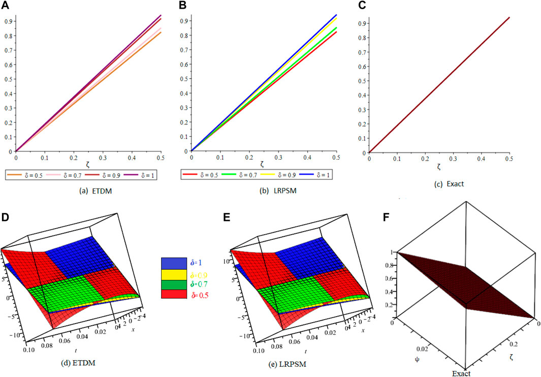
FIGURE 1. The comparison of (A,D) ETDM, (B,E) LRPSM, and (C,F) exact 2D and 3D plots, at different fractional orders of example 4.1.

FIGURE 2

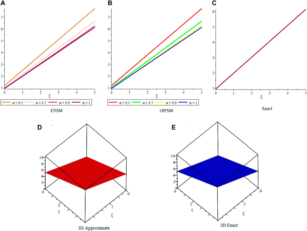
FIGURE 2. The comparison of (A) ETDM, (B) LRPSM, and (C) exact 2D plots at different-fractional-order. (D) Approximate and (E) exact 3D plots of example 4.2 at δ = 1.

FIGURE 3

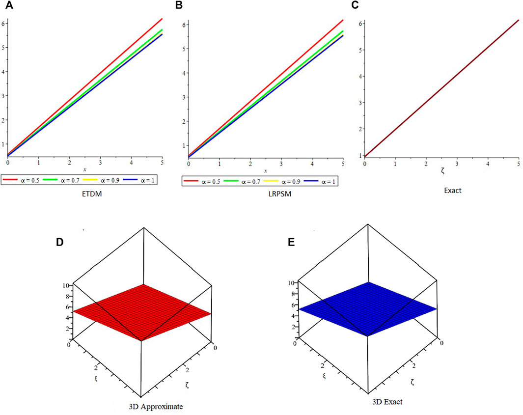
FIGURE 3. The comparison of (A) ETDM, (B) LRPSM, and (C) exact 2D plots at different-fractional-order δ. (D) Approximate and (E) exact 3D plots of example 4.3 at δ = 1.

FIGURE 4

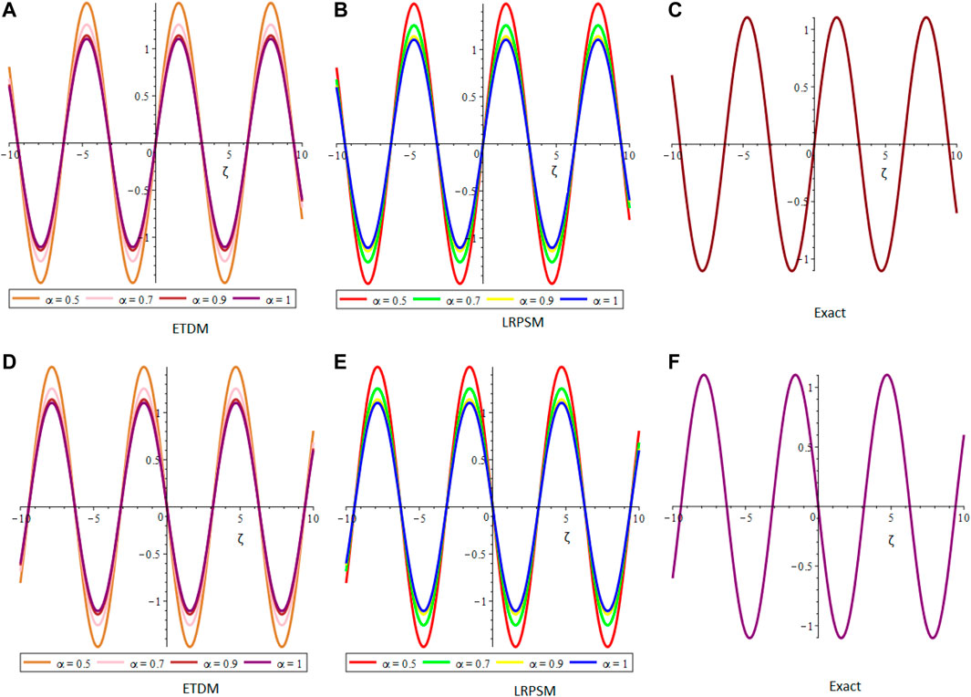
FIGURE 4. The comparison of (A,D) ETDM, (B,E) LRPSM, and (C,F) exact 2D plots of μ and ν-solution, at different fractional orders of example 4.4.

FIGURE 5

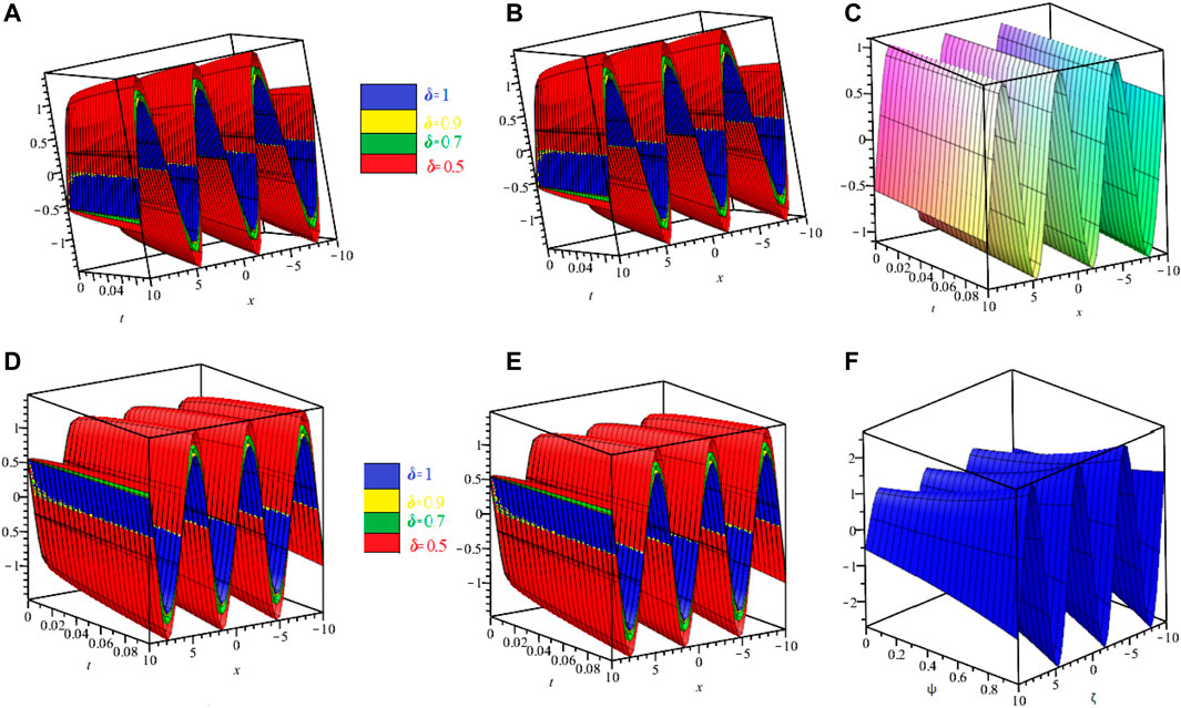
FIGURE 5. The comparison of (A,D) ETDM, (B,E) LRPSM, and (C,F) exact 3D plots of μ and ν-solution, at different fractional orders of example 4.4.

FIGURE 6

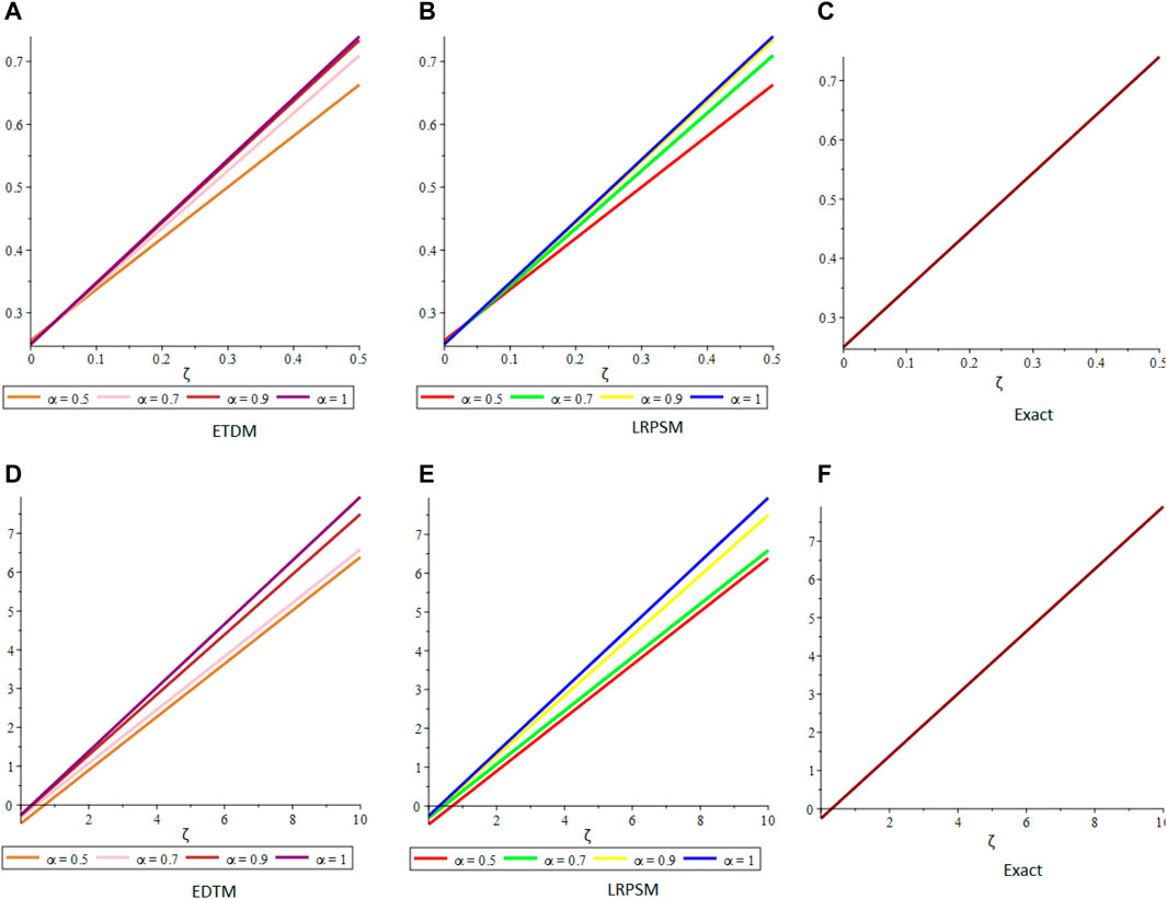
FIGURE 6. The comparison of (A,D) ETDM, (B,E) LRPSM, and (C,F) exact 2D plots of μ and ν-solution, at different fractional orders of example 4.5.

FIGURE 7

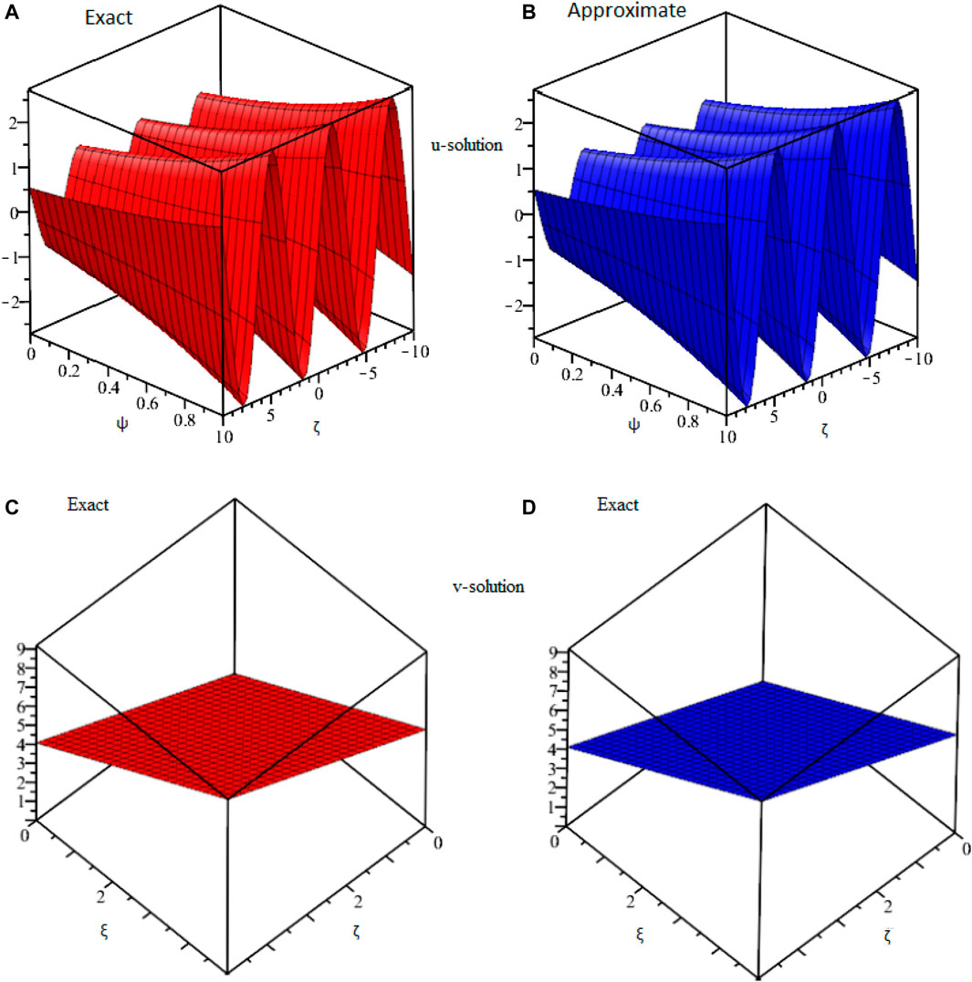
FIGURE 7. The comparison of (A,C) exact and (B,D) approximate 3D plots of μ and ν-solution, respectively, at fractional-order δ = 1 of example 4.5.

Table 1, confirm the higher accuracy of LRPSM, and ETDM at different values of space and time variables, of Example 4.1. In Table 2, the μ corresponding errors associated with ETDM and LRPSM for μ-variable at various fractional order of example 4.2 are shown. In Table 3, the error associated with LRPSM and ETDM for the μ-solution of example 4.3 at different times and spaces is calculated. Table 4, displays the absolute error for μ-solution associated with ETDM and LRPSM at different times levels and spaces of example 4.4. Table 5, displays the absolute error for ν-solution associated with ETDM and LRPSM at different times levels and spaces of example 4.4. Table 6, displays the absolute error for μ-solution associated with ETDM and LRPSM at different times levels and spaces of example 4.5. Table 7, displays the absolute error for ν-solution associated with ETDM and LRPSM at different times levels and spaces of example 4.5.

TABLE 1

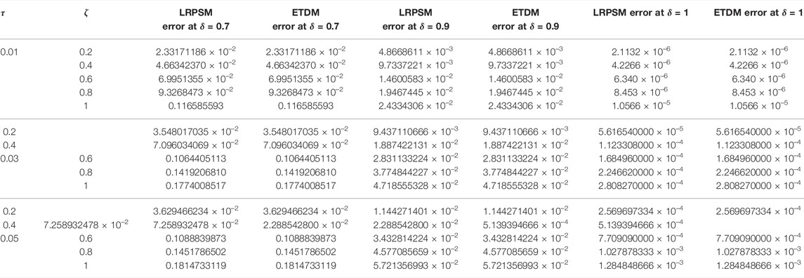
TABLE 1. Comparison of LRPSM and ETDM errors at different time levels and spaces for example 4.1

TABLE 2

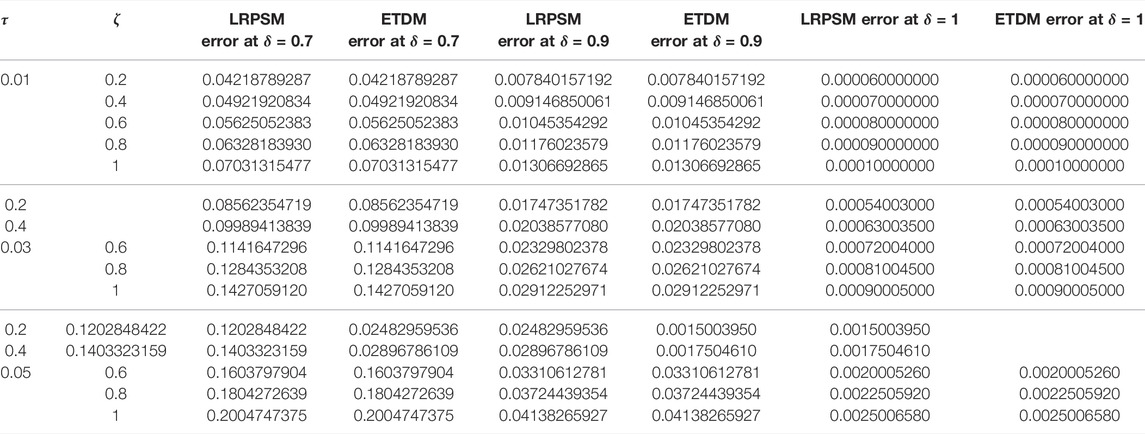
TABLE 2. Comparison of LRPSM and ETDM errors of μ(ζ, τ) solution at different time levels and spaces of example 4.2

TABLE 3

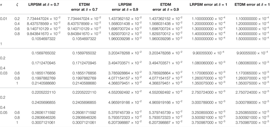
TABLE 3. Comparison of LRPSM and ETDM errors of μ(ζ, τ) solution at different time levels and spaces of example 4.3

TABLE 4

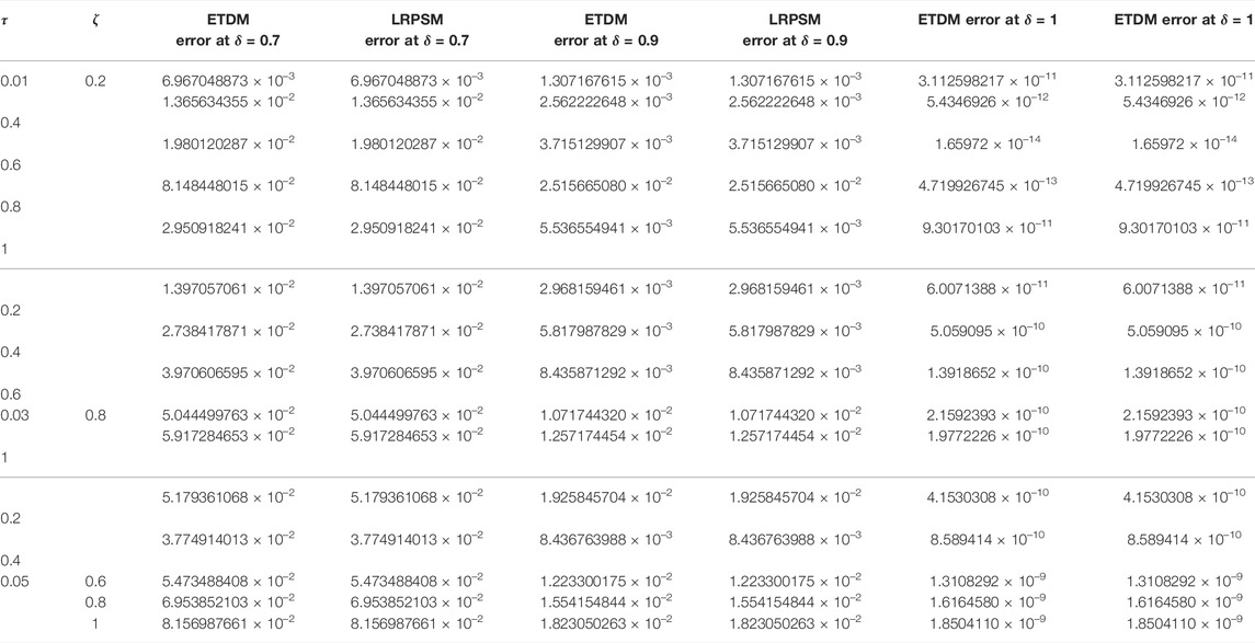
TABLE 4. Comparison of LRPSM and ETDM errors of μ(ζ, τ) solution at different time levels and spaces of example 4.4

TABLE 5

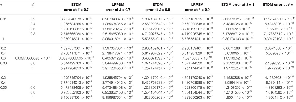
TABLE 5. Comparison of LRPSM and ETDM errors of ν(ζ, τ) solution at different time levels and spaces of example 4.4

TABLE 6

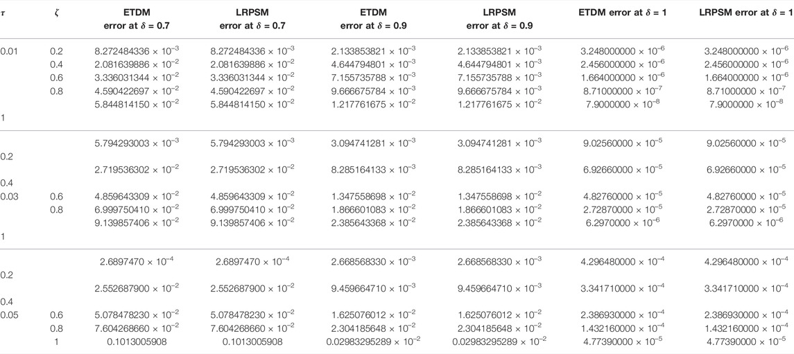
TABLE 6. Comparison of LRPSM and ETDM errors of μ(ζ, τ) solution at different time levels and spaces of example 4.5

TABLE 7

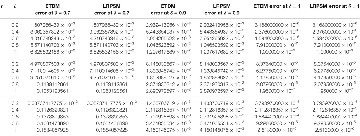
TABLE 7. Comparison of LRPSM and ETDM errors of ν(ζ, τ) solution at different time levels and spaces of example 4.5

6 Conclusion

The current article, presents the analytical solutions of one- and two-dimensional fractional Burger’s equations and their systems using efficient techniques. In this regard, the solutions of the two innovative techniques, the Laplace residual power series method (LRPS) and the Elzaki transform decomposition method (ETDM), are compared within the Caputo operator. The comparison has confirmed that the suggested techniques provide identical solutions to both fractional- and integer-order solutions of the targeted problems. For the validity and applicability of the proposed techniques, the solutions of some illustrative examples are presented. The ETDM and LRPS algorithms are developed in a very simple and straightforward manner. The calculations in each algorithm are up to the limit. The tables and graphs are presented for the best display of the obtained results and errors associated with ETDM and LRPSM. The fractional-order solutions are calculated and are represented by graphs and tables. The accuracy of the suggested techniques is calculated in terms of absolute error associated with suggested techniques. The error analysis has confirmed the higher degree of accuracy and convergence rates. The present modifications to the existing techniques have brought significant change in the field of computational mathematics. It is, therefore, suggested to implement the current techniques in various areas of science and engineering.

Data Availability Statement

The raw data supporting the conclusion of this article will be made available by the authors without undue reservation.

Author Contributions

HK: supervision. QK: methodology, Hajira: draft writing. SK: analytic calculations, MA: draft writing. PK: funding.

Funding

This research was funded by National Science, Research and Innovation Fund (NSRF), and King Mongkut’s University of Technology North Bangkok with Contract no. KMUTNB-FF-65-24.

Conflict of Interest

The authors declare that the research was conducted in the absence of any commercial or financial relationships that could be construed as a potential conflict of interest.

Publisher’s Note

All claims expressed in this article are solely those of the authors and do not necessarily represent those of their affiliated organizations or those of the publisher, the editors, and the reviewers. Any product that may be evaluated in this article, or claim that may be made by its manufacturer, is not guaranteed or endorsed by the publisher.

References

1 Leibniz GW. Letter from Hanover, Germany to GFA L’Hospital. Mathematische Schriften (1849). p. 301–2.

Google Scholar

2 Podlubny I. Fractional Differential Equations: An Introduction to Fractional Derivatives, Fractional Differential Equations, to Methods of Their Solution and Some of Their Applications. Elsevier (1998).

Google Scholar

3 Samko SG. Fractional Integrals and Derivatives, Theory and Applications. Minsk: Nauka I Tekhnika (1987).

Google Scholar

4 Kilbas AA, Srivastava HM, Trujillo JJ. Theory and Applications of Fractional Differential Equations, 204. Elsevier (2006).

Google Scholar

5 Hilfer R. Applications of Fractional Calculus in Physics. World Scientific (2000).

Google Scholar

6 Magin RL. Fractional Calculus in Bioengineering, Part 3. Crit Rev Biomed Eng (2004) 32(1):195–377. doi:10.1615/critrevbiomedeng.v32.i34.10

PubMed Abstract | CrossRef Full Text | Google Scholar

7 Zhao J, Tang B, Kumar S, Hou Y. The Extended Fractional Subequation Method for Nonlinear Fractional Differential Equations. Mathematical Problems in Engineering (2012).

Google Scholar

8 Atangana A, Kılıçman A. A Possible Generalization of Acoustic Wave Equation Using the Concept of Perturbed Derivative Order. Math Probl Eng (2013) 2013(1):1–6. doi:10.1155/2013/696597

CrossRef Full Text | Google Scholar

9 Atangana A, Secer A. January. The Time-Fractional Coupled-Korteweg-De-Vries Equations. In: Abstract and Applied Analysis, 2013. Hindawi (2013). doi:10.1155/2013/947986

CrossRef Full Text | Google Scholar

10 Zaslavsky GM, Zaslavskij GM. Hamiltonian Chaos and Fractional Dynamics. Oxford University Press on Demand (2005).

Google Scholar

11 Ahmad B, Nieto JJ. Existence Results for Nonlinear Boundary Value Problems of Fractional Integrodifferential Equations with Integral Boundary Conditions. Boundary value Probl (2009) 2009:1–11. doi:10.1155/2009/708576

CrossRef Full Text | Google Scholar

12 Caputo M. Linear Models of Dissipation Whose Q Is Almost Frequency Independent--II. Geophys J Int (1967) 13(5):529–39. doi:10.1111/j.1365-246x.1967.tb02303.x

CrossRef Full Text | Google Scholar

13 Turut V, Güzel N. On Solving Partial Differential Eqauations of Fractional Order by Using the Variational Iteration Method and Multivariate Padé Approximation (2013).

Google Scholar

14 He JH. Some Applications of Nonlinear Fractional Differential Equations and Their Approximations. Bull Sci Technol (1999) 15(2):86–90.

Google Scholar

15 Scher H, Montroll EW. Anomalous Transit-Time Dispersion in Amorphous Solids. Phys Rev B (1975) 12(6):2455–77. doi:10.1103/physrevb.12.2455

CrossRef Full Text | Google Scholar

16 Nigmatullin RR. The Realization of the Generalized Transfer Equation in a Medium with Fractal Geometry. Phys Stat Sol (B) (1986) 133(1):425–30. doi:10.1002/pssb.2221330150

CrossRef Full Text | Google Scholar

17 Müller H-P, Kimmich R, Weis J. NMR Flow Velocity Mapping in Random Percolation Model Objects: Evidence for a Power-Law Dependence of the Volume-Averaged Velocity on the Probe-Volume Radius. Phys Rev E (1996) 54(5):5278–85. doi:10.1103/physreve.54.5278

CrossRef Full Text | Google Scholar

18 Amblard F, Maggs AC, Yurke B, Pargellis AN, Leibler S. Subdiffusion and Anomalous Local Viscoelasticity in Actin Networks. Phys Rev Lett (1996) 77(21):4470–3. doi:10.1103/physrevlett.77.4470

PubMed Abstract | CrossRef Full Text | Google Scholar

19 Barkai E, Metzler R, Klafter J. From Continuous Time Random Walks to the Fractional Fokker-Planck Equation. Phys Rev E (2000) 61(1):132–8. doi:10.1103/physreve.61.132

CrossRef Full Text | Google Scholar

20 Henry BI, Wearne SL. Fractional Reaction–Diffusion. Physica A: Stat Mech its Appl (2000) 276(3-4):448–55. doi:10.1016/s0378-4371(99)00469-0

CrossRef Full Text | Google Scholar

21 Coimbra CFM. Mechanics with Variable-Order Differential Operators. Ann Phys (2003) 12(11-12):692–703. doi:10.1002/andp.200310032

CrossRef Full Text | Google Scholar

22 Diaz G, Coimbra CFM. Nonlinear dynamics and control of a variable order oscillator with application to the van der Pol equation. Nonlinear Dyn (2009) 56(1):145–57. doi:10.1007/s11071-008-9385-8

CrossRef Full Text | Google Scholar

23 Ingman D, Suzdalnitsky J. Control of Damping Oscillations by Fractional Differential Operator with Time-dependent Order. Computer Methods Appl Mech Eng (2004) 193(52):5585–95. doi:10.1016/j.cma.2004.06.029

CrossRef Full Text | Google Scholar

24 Kivshar YS, Agrawal GP. Optical Solitons: From Fibers to Photonic Crystals. Academic Press (2003).

Google Scholar

25 Dehghan M, Safarpoor M. The Dual Reciprocity Boundary Elements Method for the Linear and Nonlinear Two-Dimensional Time-Fractional Partial Differential Equations. Math Meth Appl Sci (2016) 39(14):3979–95. doi:10.1002/mma.3839

CrossRef Full Text | Google Scholar

26 Daftardar-Gejji V, Jafari H. Solving a Multi-Order Fractional Differential Equation Using Adomian Decomposition. Appl Mathematics Comput (2007) 189(1):541–8. doi:10.1016/j.amc.2006.11.129

CrossRef Full Text | Google Scholar

27 He J-H. An Elementary Introduction to the Homotopy Perturbation Method. Comput Mathematics Appl (2009) 57(3):410–2. doi:10.1016/j.camwa.2008.06.003

CrossRef Full Text | Google Scholar

28 Mohebbi A, Abbaszadeh M, Dehghan M. The Use of a Meshless Technique Based on Collocation and Radial Basis Functions for Solving the Time Fractional Nonlinear Schrödinger Equation Arising in Quantum Mechanics. Eng Anal Boundary Elem (2013) 37(2):475–85. doi:10.1016/j.enganabound.2012.12.002

CrossRef Full Text | Google Scholar

29 Harris FE. Mathematics for Physical Science and Engineering: Symbolic Computing Applications in Maple and Mathematica. Academic Press (2014).

Google Scholar

30 Salahshour S, Allahviranloo T, Abbasbandy S. Solving Fuzzy Fractional Differential Equations by Fuzzy Laplace Transforms. Commun Nonlinear Sci Numer Simulation (2012) 17(3):1372–81. doi:10.1016/j.cnsns.2011.07.005

CrossRef Full Text | Google Scholar

31 Baseri A, Babolian E, Abbasbandy S. Normalized Bernstein Polynomials in Solving Space-Time Fractional Diffusion Equation. Adv Difference Equations (2017) 2017(1):1–25. doi:10.1186/s13662-017-1401-1

CrossRef Full Text | Google Scholar

32 Wang L, Ma Y, Meng Z. Haar Wavelet Method for Solving Fractional Partial Differential Equations Numerically. Appl Math Comput (2014) 227:66–76.

CrossRef Full Text | Google Scholar

33 Jafari H, Nazari M, Baleanu D, Khalique CM. A New Approach for Solving a System of Fractional Partial Differential Equations. Comput Mathematics Appl (2013) 66(5):838–43. doi:10.1016/j.camwa.2012.11.014

CrossRef Full Text | Google Scholar

34 Chen Y, Sun Y, Liu L. Numerical Solution of Fractional Partial Differential Equations with Variable Coefficients Using Generalized Fractional-Order Legendre Functions. Appl Mathematics Comput (2014) 244:847–58. doi:10.1016/j.amc.2014.07.050

CrossRef Full Text | Google Scholar

35 Jassim HK. January. The Approximate Solutions of Three-Dimensional Diffusion and Wave Equations within Local Fractional Derivative Operator. In: Abstract and Applied Analysis, 2016. Hindawi (2016). doi:10.1155/2016/2913539

CrossRef Full Text | Google Scholar

36 Biswas A, Bhrawy AH, Abdelkawy MA, Alshaery AA, Hilal EM. Symbolic Computation of Some Nonlinear Fractional Differential Equations. Rom J Phys (2014) 59(5-6):433–42.

Google Scholar

37 Bhrawy AH. A Jacobi Spectral Collocation Method for Solving Multi-Dimensional Nonlinear Fractional Sub-diffusion Equations. Numer Algor (2016) 73(1):91–113. doi:10.1007/s11075-015-0087-2

CrossRef Full Text | Google Scholar

38 Zhang Y-Z, Yang A-M, Long Y. Initial Boundary Value Problem for Fractal Heat Equation in the Semi-infinite Region by Yang-Laplace Transform. Therm Sci (2014) 18(2):677–81. doi:10.2298/tsci130901152z

CrossRef Full Text | Google Scholar

39 Bhrawy AH. January. A New Spectral Algorithm for Time-Space Fractional Partial Differential Equations with Subdiffusion and Superdiffusion. Proc Rom Acad Ser A (2016) 17(No. 1):39–47.

Google Scholar

40 Maitama S, Abdullahi I. A New Analytical Method for Solving Linear and Nonlinear Fractional Partial Differential Equations. Progr Fract Differ Appl (2016) 2(4):247–56. doi:10.18576/pfda/020402

CrossRef Full Text | Google Scholar

41 Zhang Y, Baleanu D, Yang X. On a Local Fractional Wave Equation under Fixed Entropy Arising in Fractal Hydrodynamics. Entropy (2014) 16(12):6254–62. doi:10.3390/e16126254

CrossRef Full Text | Google Scholar

42 Bhrawy AH. January. A New Legendre Collocation Method for Solving a Two-Dimensional Fractional Diffusion Equation. In: Abstract and Applied Analysis, 2014. Hindawi (2014). doi:10.1155/2014/636191

CrossRef Full Text | Google Scholar

43 Yusufoglu E, Bekir A. Numerical Simulation of Equal-Width Wave Equation. Comput Math Appl (2007) 54(7-8):1147–53. doi:10.1016/j.camwa.2006.12.080

CrossRef Full Text | Google Scholar

44 Yusufoglu E, Bekir A. The Variational Iteration Method for Solitary Patterns Solutions of gBBM Equation. Phys Lett A (2007) 367(6):461–4. doi:10.1016/j.physleta.2007.03.045

CrossRef Full Text | Google Scholar

45 Bekir A. On Traveling Wave Solutions to Combined KdV-mKdV Equation and Modified Burgers-KdV Equation. Commun Nonlinear Sci Numer Simulation (2009) 14(4):1038–42. doi:10.1016/j.cnsns.2008.03.014

CrossRef Full Text | Google Scholar

46 Kaplan M, Akbulut A. The Analysis of the Soliton-type Solutions of Conformable Equations by Using Generalized Kudryashov Method. Opt Quan Electronics (2021) 53(9):1–21. doi:10.1007/s11082-021-03144-y

CrossRef Full Text | Google Scholar

47 Melike Kaplan M, San S, Sait San A. On the Exact Solutions and Conservation Laws to the Benjamin-Ono Equation. jaac (2018) 8(1):1–9. doi:10.11948/2018.1

CrossRef Full Text | Google Scholar

48 Bateman H. Some Recent Researches on the Motion of Fluids. Mon Wea Rev (1915) 43(4):163–70. doi:10.1175/1520-0493(1915)43<163:srrotm>2.0.co;2

CrossRef Full Text | Google Scholar

49 Whitham GB. Linear and Nonlinear Waves, 42. John Wiley & Sons (2011).

Google Scholar

50 E W, Khanin K, Mazel A, Sinai Y. Invariant Measures for Burgers Equation with Stochastic Forcing. Ann Mathematics (2000) 151:877–960. doi:10.2307/121126

CrossRef Full Text | Google Scholar

51 Basto M, Semiao V, Calheiros F. Dynamics and Synchronization of Numerical Solutions of the Burgers Equation. J Comput Appl Math (2009) 231(2):793–806. doi:10.1016/j.cam.2009.05.003

CrossRef Full Text | Google Scholar

52 Rashidi MM, Erfani E. New Analytical Method for Solving Burgers' and Nonlinear Heat Transfer Equations and Comparison with HAM. Computer Phys Commun (2009) 180(9):1539–44. doi:10.1016/j.cpc.2009.04.009

CrossRef Full Text | Google Scholar

53 Wazwaz AM. Partial Differential Equations. CRC Press (2002).

Google Scholar

54 Cole JD. On a Quasi-Linear Parabolic Equation Occurring in Aerodynamics. Quart Appl Math (1951) 9(3):225–36. doi:10.1090/qam/42889

CrossRef Full Text | Google Scholar

55 Ozis T, Ozdes A. A Direct Variational Methods Applied to Burgers' Equation. J Comput Appl Math (1996) 71(2):163–75. doi:10.1016/0377-0427(95)00221-9

CrossRef Full Text | Google Scholar

56 Jaiswal S. Study of Some Transport Phenomena Problems in Porous media (Doctoral Dissertation) (2017).

Google Scholar

57 Evans DJ, Abdullah AR. The Group Explicit Method for the Solution of Burger's Equation. Computing (1984) 32(3):239–53. doi:10.1007/bf02243575

CrossRef Full Text | Google Scholar

58 Mittal RC, Singhal P. Numerical Solution of Burger's Equation. Commun Numer Meth Engng (1993) 9(5):397–406. doi:10.1002/cnm.1640090505

CrossRef Full Text | Google Scholar

59 Caldwell J, Wanless P, Cook AE. A Finite Element Approach to Burgers' Equation. Appl Math Model (1981) 5(3):189–93. doi:10.1016/0307-904x(81)90043-3

CrossRef Full Text | Google Scholar

60 Kurt A, Cenesiz Y, Tasbozan O. Exact Solution for the Conformable Burgers’ Equation by the Hopf-Cole Transform. Cankaya Univ J Sci Eng (2016) 13(2):18–23.

Google Scholar

61 Inc M. The Approximate and Exact Solutions of the Space- and Time-Fractional Burgers Equations with Initial Conditions by Variational Iteration Method. J Math Anal Appl (2008) 345(1):476–84. doi:10.1016/j.jmaa.2008.04.007

CrossRef Full Text | Google Scholar

62 Esen A, Yagmurlu NM, Tasbozan O. Approximate Analytical Solution to Time-Fractional Damped Burger and Cahn-Allen Equations. Appl Math Inf Sci (2013) 7(5):1951–6. doi:10.12785/amis/070533

CrossRef Full Text | Google Scholar

63 Esen A, Tasbozan O. Numerical Solution of Time Fractional Burgers Equation by Cubic B-Spline Finite Elements. Mediterr J Math (2016) 13(3):1325–37. doi:10.1007/s00009-015-0555-x

CrossRef Full Text | Google Scholar

64 Elzaki TM. The New Integral Transform Elzaki Transform. Glob J Pure Appl Math (2011) 7(1):57–64.

Google Scholar

65 Adomian G. A Review of the Decomposition Method in Applied Mathematics. J Math Anal Appl (1988) 135(2):501–44. doi:10.1016/0022-247x(88)90170-9

CrossRef Full Text | Google Scholar

66 Elzaki TM. On the New Integral Transform”Elzaki Transform”Fundamental Properties Investigations and Applications. Glob J Math Sci Theor Pract (2012) 4(1):1–13.

Google Scholar

67 Neamaty A, Agheli B, Darzi R. Applications of Homotopy Perturbation Method and Elzaki Transform for Solving Nonlinear Partial Differential Equations of Fractional Order. J Nonlin Evolut Equat Appl (2016) 2015(6) 91–104.

Google Scholar

68 Jena RM, Chakraverty S. Solving Time-Fractional Navier–Stokes Equations Using Homotopy Perturbation Elzaki Transform. SN Appl Sci (2019) 1(1):1–13. doi:10.1007/s42452-018-0016-9

CrossRef Full Text | Google Scholar

69 Sedeeg AKH. A Coupling Elzaki Transform and Homotopy Perturbation Method for Solving Nonlinear Fractional Heat-like Equations. Am J Math Comput Model (2016) 1:15–20.

Google Scholar

70 Eriqat T, El-Ajou A, Oqielat Ma. N, Al-Zhour Z, Momani S. A New Attractive Analytic Approach for Solutions of Linear and Nonlinear Neutral Fractional Pantograph Equations. Chaos, Solitons & Fractals (2020) 138:109957. doi:10.1016/j.chaos.2020.109957

CrossRef Full Text | Google Scholar

71 Alquran M, Ali M, Alsukhour M, Jaradat I. Promoted Residual Power Series Technique with Laplace Transform to Solve Some Time-Fractional Problems Arising in Physics. Results Phys (2020) 19:103667. doi:10.1016/j.rinp.2020.103667

CrossRef Full Text | Google Scholar

72 Elzaki TM. Elzaki and Sumudu Transforms for Solving Some Differential Equations. Glob J Pure Appl Mathematics (2012) 8(2):167–173.

Google Scholar